From Pixel Receptive Fields to Ground Spans: GSD-Conditioned Cross-Resolution Feature Alignment for Photovoltaic Detection and Segmentation

Highlights

What are the main findings?

• CRFA-PVNet uses GSD-conditioned feature alignment to detect and segment PV installations in satellite, aerial, and UAV imagery. A single model is jointly trained on data from all three tiers. CRFA-PVNet achieves the highest OBB mAP50 and mask IoU among the evaluated methods across all three GSD tiers.
• With proposal-guided local mask refinement, CRFA-PVNet reaches 41.3 FPS with 3.74 GB peak memory on an NVIDIA Jetson TX2 when deployed with TensorRT FP16. Its macro OBB mAP50 and macro mask IoU are each only 0.002 lower than with TensorRT FP32.

What is the implication of the main finding?

• The larger gains at the coarsest tier are consistent with the physical ground-span formulation, supporting the use of GSD as an explicit conditioning cue for cross-resolution feature learning.
• Restricting dense mask parsing to oriented PV proposals reduces mask computation over background regions, supporting a resource-aware design for embedded PV detection and segmentation.

Abstract

Photovoltaic (PV) inventories with explicit location and extent are needed for energy accounting, distribution-grid planning, and asset monitoring. However, the ground sampling distance (GSD) of different sources spans nearly an order of magnitude, so a sampling window of fixed pixel size covers 64 times more ground at 0.8 m than at 0.1 m. This physical-scale discrepancy can weaken cross-resolution generalization. To address this, this paper proposes CRFA-PVNet, a physically guided cross-resolution feature alignment network for PV detection and segmentation, which describes the receptive field in ground units rather than in pixels. First, a physical receptive-field formulation quantifies the physical-support gap between GSD conditions, while a normalized discrepancy between spatially aligned fusion features defines the cross-resolution representation error. Second, CRFA formulates fusion-stage feature reassembly as a GSD-conditioned operator: effective GSD modulates the spatial evidence used to generate content-aware local aggregation kernels, making the reassembly weights joint functions of image content and physical sampling scale. Third, a proposal-guided local mask refinement pipeline restricts boundary parsing to oriented proposals and lowers inference cost on embedded hardware. Fourth, a spatially disjoint validation protocol, with the buffer distance set from Moran’s I and semivariogram range, limits spatial information leakage. One jointly trained parameter set serves 0.1, 0.3, and 0.8 m imagery. The largest gains occur on the 0.8 m satellite imagery. OBB mAP50 reaches 0.849, and mask IoU reaches 0.764. These results are consistent with the physical ground-span analysis. On an NVIDIA Jetson TX2, TensorRT FP16 reaches 41.3 FPS with 3.74 GB peak memory and a 0.002 macro accuracy loss.

1. Introduction

Photovoltaic power generation has developed from a supplementary energy technology into a major component of the global energy system. By the end of 2025, cumulative PV capacity had approached 2.97 TW worldwide, after approximately 0.70 TW was added in a single year [1]. China alone had reached 1.20 TW of PV capacity, including 0.53 TW of distributed installations [2]. Distributed PV represented 44% of China’s cumulative PV capacity and nearly half of its annual additions [2]. These data indicate that photovoltaic systems have become a large-scale and fast-evolving component of energy infrastructure. Distributed PV installations are widely deployed across industrial facilities, residential buildings, rural settlements, and other heterogeneous environments.

This rapid expansion creates a spatial information challenge in addition to an energy generation challenge. Aggregate capacity statistics indicate how much PV capacity has been installed, but they do not reveal the location, spatial extent, or boundary changes of individual installations. Manual counting and statistics cannot meet the requirements for update efficiency and spatial accuracy of current PV deployment, especially for geographically dispersed PV systems. Multi-scale remote-sensing techniques can serve as an effective complement to conventional manual-based approaches. By acquiring precise location and spatial-extent information of individual PV installations, they can support installed-capacity assessment, PV resource accounting, infrastructure inspection, and distribution-grid planning.

Satellite imagery enables repeated wide-area observation, aerial imagery supports regional fine-grained mapping, and UAV imagery provides detailed panel structures and local boundaries. However, imagery from these sources exhibits substantial differences in ground sampling distance. The same PV array may be presented at different sizes and resolutions. More importantly, the same pixel-level receptive field corresponds to different physical ground areas. In UAV images, the receptive field can capture the structure of individual PV panels. In satellite images, it may cover multiple PV panels together with rooftops and other background interference. Therefore, physical scale information should be explicitly incorporated into cross-resolution feature learning.

Early studies relied on spectral or hyperspectral cues for PV panel detection and power generation estimation [3]. The public aerial PV dataset and the AIR-PV benchmark test have enhanced the reproducibility of subsequent supervised PV research [4,5]. Current algorithms use multi-scale convolutional representations [6] and attention-based context modeling [7], while related context-aware multi-scale designs have also been explored [8]. However, their sampling fields are typically defined in image coordinates. Although GSD can be explicitly encoded, the remaining question is how physical scale should condition feature aggregation during cross-resolution fusion. This distinction is important when one model is applied to satellite, aerial, and UAV imagery.

This issue is particularly prominent in the identification of PV arrays. PV arrays are characterized by being regular, elongated, and having thin boundaries which are easily mistaken for roof edges, shadows, or metal supports during identification. In satellite images, the boundaries of PV panels often blend with the background, whereas UAV images can reveal details such as cell borders and local reflections. Previous studies on aerial images and heterogeneous remote-sensing images also indicated that the appearance of PV arrays varies significantly under different resolutions and scene conditions [9,10]. As a result, a fixed pixel receptive field captures different parts of an object across different tiers, resulting in mask fragmentation, omission in small regions, and unstable bounding box regression.

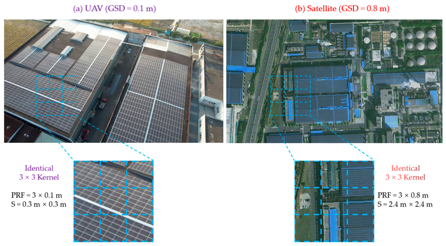
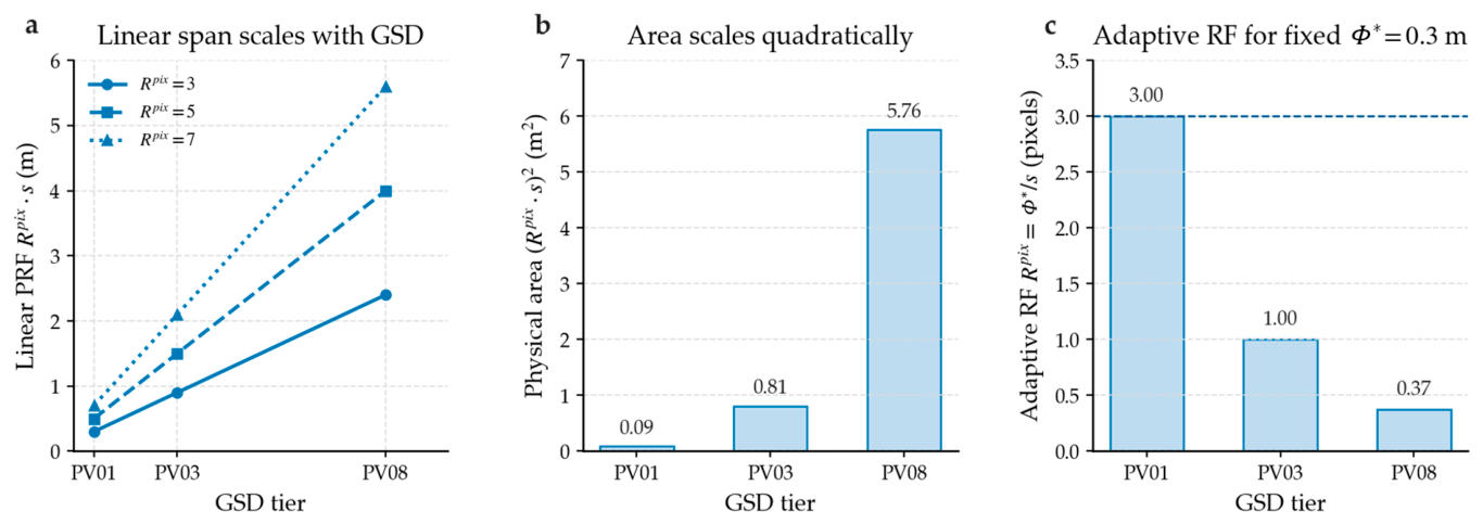
Figure 1 illustrates this phenomenon. A 3 × 3 sampling window spans 0.3 m × 0.3 m in the 0.1 m UAV tier, capturing local textures or narrow boundaries, while in the 0.8 m satellite tier, the same window spans 2.4 m × 2.4 m, 64 times the area. It mixes several PV panels with cluttered background. Fixed pixel-level receptive fields could not observe equivalent evidence across different tiers, which helps explain the instability of cross-resolution transfer.

Efficient deployment is the second challenge. Large-area PV detection and segmentation possibly need to run on airborne or field-side devices with limited memory and power, rather than simply on workstations. Dense full-frame segmentation may lead to the model wasting a significant amount of computation in areas without PV arrays, further giving rise to the issue of exceeding the available memory budget on embedded devices. A deployable system must strike a balance between localization accuracy, extraction quality, and controllable operation time.

Spatial autocorrelation also complicates the evaluation. Adjacent patches have similar solar illumination conditions, background materials, and building styles. Simple random-patch splitting may place similar spatial contexts in both training and test sets. The results derived from this may overstate the performance across different regions.

This paper proposes CRFA-PVNet to address the cross-resolution mismatch in multi-scale PV images. Building on prior GSD-aware research, CRFA uses effective GSD specifically at the multi-scale feature-fusion stage to condition spatial gating and content-aware reassembly-weight prediction. This operator-level design propagates physical scale into the local-kernel generation process. The physical receptive-field formulation links pixel-level sampling to physical ground span, while the conditioned reassembly operator allows one shared parameter set to adapt feature aggregation across satellite, aerial, and UAV imagery.

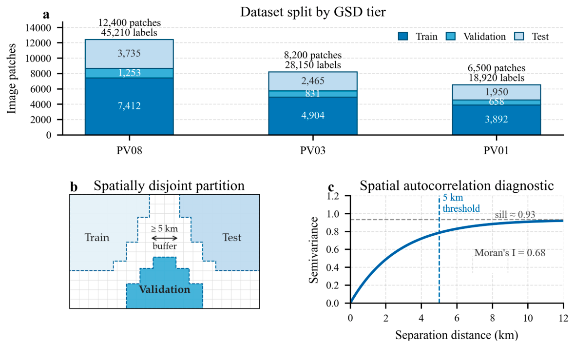
To optimize edge deployment, this paper uses a proposal-guided local mask refinement pipeline in CRFA-PVNet. Before refining masks in selected local regions, it first locates oriented PV candidate regions. This could avoid dense prediction in large background areas and reduce the inference burden on edge devices. The dataset is partitioned with a spatially disjoint protocol based on Moran’s I and semivariogram analysis, with a minimum 5-km buffer between the training, validation, and testing subsets.

In order to isolate the effect of GSD, we use controlled same-scene resampling, GSD-input interventions, and unseen intermediate-GSD tests to evaluate the role of physical-scale conditioning in feature alignment and cross-resolution prediction.

The main contributions of this paper are as follows.

(1) A GSD-conditioned feature-reassembly operator is developed for cross-resolution PV representation. The physical receptive field expresses each sampling window in ground units, providing an interpretable link between pixel support and physical ground span. Within CRFA, effective GSD is encoded and interacts with spatial features before local-kernel prediction, transforming content-only reassembly $K(X)$ into physical-scale-conditioned reassembly $K(X,s_{\mathrm{e}\mathrm{f}\mathrm{f}})$. This allows one shared parameter set to adapt feature aggregation across imagery with different spatial resolutions. It also supports oriented PV detection and proposal-guided mask segmentation. The largest gains are observed on the 0.8 m tier, the OBB mAP50 increases by 0.042 and the mask IoU rises by 0.152.

(2) A Proposal-Guided Local Mask Refinement pipeline is designed for deployable PV detection and segmentation. It locates oriented candidate regions and refines masks only within the selected local regions. Affine coordinate mapping and memory-aware RoI batching keep dense parsing off large background areas and stabilize memory usage during edge inference. On an NVIDIA Jetson TX2, TensorRT FP16 reaches 41.3 FPS with 3.74 GB peak memory and a 0.002 macro accuracy loss.

(3) A spatially disjoint evaluation protocol is adopted to limit neighborhood leakage. Moran’s I and semivariogram analysis set the buffer distance between the training, validation, and test subsets. Random partitioning gives a validation-test gap of +0.150 for YOLOv10-B, while the spatially disjoint protocol reduces it to +0.006. The reported results therefore give a more conservative estimate of cross-regional performance.

The remainder of the paper is organized as follows. Section 2 reviews related work. Section 3 describes the dataset, spatial partitioning protocol, and CRFA-PVNet framework. Section 4 presents the results and analysis. Section 5 concludes the paper.

2. Related Work

2.1. Multi-Scale and Cross-Resolution Feature Representation

Scale variation is a common problem in remote-sensing images. A target may occupy only a few pixels in one image but many pixels in another. Scale-space theory first described how image structures change across scale [11]. Spatial pyramid pooling and feature pyramid networks later combined features from different resolutions for recognition and detection [12,13]. Atrous spatial pyramid pooling expands the sampling range with parallel dilated convolutions [6]. These methods improve multi-scale representation, but they describe scale in pixels rather than in physical ground distance.

This limitation becomes obvious when images come from different sources with different scales. The same PV array may be clear in a UAV image but blurred in a satellite image. A receptive field that captures panel texture in the UAV image may cover several arrays and nearby background in the satellite image. Multi-scale modules can combine image features, but they usually do not state how much ground each pixel represents. Sensor blur and background mixing make this difference larger across platforms.

Adaptive sampling provides another way to handle geometric variation. Deformable convolution learns sampling offsets from local image content [14]. CARAFE predicts local reassembly kernels during upsampling [15]. Both are useful for PV boundaries, but their sampling decisions are still based on appearance. They do not use GSD to describe the physical scale of the image.

External information can also guide representation learning. Physics-informed learning incorporates known physical structure into data-driven models [16]. Sinusoidal and Fourier encodings convert a scalar input into a feature representation that a network can use [17]. For PV remote sensing, GSD is a practical physical input because it specifies the ground size of a pixel. Previous GSD-aware methods already use GSD explicitly. They differ in where GSD enters the network and how it influences feature learning.

GSDet estimates GSD from the input image, combines it with RoI dimensions to infer physical object size, and reweights category-specific detection features [18]. Scale-MAE uses GSD to scale sinusoidal positional encoding during self-supervised pretraining for multiscale geospatial representation learning [19]. GSDDet learns GSD-related features from the input image and couples them with an attention-based detector to reduce cross-scale category confusion [20]. These studies establish GSD as an informative physical-scale prior. However, their conditioning is applied to RoI-level detection, positional encoding for pretraining, or detector attention, rather than to the content-aware feature-reassembly pathway at the multi-scale fusion stage.

Table 1. Positioning of GSD-aware methods according to the source, injection position, conditioned operation, and task.

Method	GSD Source	Injection Position	GSD-Conditioned Operation	Learning Task and Output
GSDet	Estimated from input image	RoI and instance level	Physical-size reasoning and category-feature reweighting	Supervised object detection
Scale-MAE	Image-scale metadata	Transformer positional encoding	Scale-aware sinusoidal position representation	Self-supervised pretraining and downstream representation
GSDDet	Learned from input image	Detector attention pathway	GSD-feature coupling for cross-scale category discrimination	Supervised object detection
CRFA-PVNet	Measured effective GSD	Multi-scale feature-fusion stage	Spatial gating and content-aware local feature reassembly	Oriented PV detection and proposal-guided mask segmentation

summarizes the GSD source, injection position, conditioned operation, and task output of these methods and CRFA-PVNet.

CRFA-PVNet differs in both the injection position of GSD and the operation that it conditions. It injects effective GSD into the local-kernel generation pathway at the multi-scale fusion stage. The reassembly weights are jointly determined by image content and physical sampling scale. A shared parameter set therefore adapts feature aggregation across images with different spatial resolutions. The aligned features support oriented PV detection and proposal-guided mask segmentation.

2.2. Efficient PV Detection and Segmentation

PV extraction has been studied using hyperspectral, aerial, satellite, and heterogeneous remote-sensing images. Early hyperspectral and high-resolution aerial studies showed that supervised learning can identify PV arrays [3,9]. DeepSolar expanded large-scale PV mapping, while AIR-PV provided a dedicated benchmark for reproducible evaluation [5,21]. Sentinel-2 and heterogeneous-image studies extended PV extraction to additional sensors and scene conditions [10,22]. Detection locates arrays, whereas segmentation provides boundaries for area estimation.

PV arrays are often elongated, dense, and rotated. As a result, oriented detection is more suitable than horizontal-box detection. RoI Transformer, ReDet, Oriented R-CNN, and R3Det represent established two-stage and refinement-based approaches for rotated objects in aerial images [23,24,25,26]. S²A-Net aligns convolutional features with refined oriented anchors, whereas Rotated RTMDet extends an efficient single-stage detector to rotated localization [27,28]. Together, these methods provide representative comparisons across two-stage, feature-alignment, and modern dense oriented-detection paradigms.

Real-time detectors are important when PV detection and segmentation must run on limited hardware. YOLOv9, YOLOv10, and RT-DETR provide representative fast localization baselines [29,30,31]. They can locate PV arrays efficiently, but they do not produce the masks needed for area estimation or detailed inspection.

Segmentation provides this boundary information. DeepLab and Mask2Former are widely used dense-prediction frameworks [6,32]. Remote-sensing segmentation models further improve their use on earth-observation images [33]. Mask R-CNN and PointRend show that instance processing and local refinement can improve boundary quality [34,35]. However, full-frame segmentation remains costly when most pixels do not contain PV arrays.

Edge deployment also depends on how computation is allocated. MobileNets, ShuffleNet V2, FasterNet, and MobileNetV2 use different strategies to reduce computational cost of vision models [36,37,38,39]. Their common lesson is that parameter count alone does not determine runtime. For PV detection and segmentation, it is also useful to avoid running a fine mask branch over large background regions. This motivates the local refinement pipeline used in this paper.

2.3. Spatial Autocorrelation and Reliable Evaluation

Remote-sensing samples are rarely spatially independent, which makes evaluation difficult. Tobler’s first law states that nearby locations tend to be more related than distant locations [40]. Neighboring image tiles can share land cover, illumination, roof materials, and local layout. A random split may therefore place highly similar patches in both the training and test sets.

Spatial autocorrelation provides a way to measure this dependence. Moran’s I is a global statistic for spatial correlation [41]. Cliff and Ord established its broader interpretation [42], and geostatistical analysis describes how correlation changes with distance [43]. These tools help determine whether nearby samples may bias validation.

Spatial dependence affects model assessment directly. Geostatistical analysis can estimate the correlation range, and blockCV provides geographically separated validation folds [43,44]. Remote-sensing studies have reported biased accuracy estimates when training and test areas are spatially dependent [45,46]. For PV detection and segmentation, spatial separation is needed when the goal is to assess transfer to a new region.

This paper first analyzes spatial autocorrelation and then defines a spatially disjoint validation protocol. The protocol reduces direct overlap between nearby regions and gives a more conservative estimate of cross-regional performance.

3. Methodology

This section presents the PV data, the spatial partitioning protocol, and CRFA-PVNet. It then explains the physical receptive field, the CRFA module, and the proposal-guided local mask refinement pipeline.

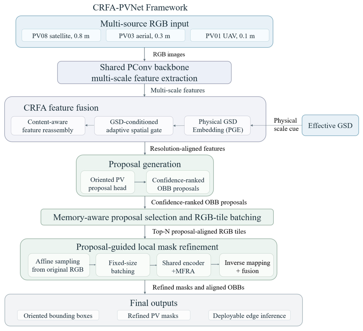
Figure 2 presents the overall CRFA-PVNet architecture and its evaluation setting.

Figure 2 summarizes the full processing flow. Multi-source RGB images are first processed by a shared backbone to obtain multi-scale features. The effective GSD conditions feature fusion through Physical GSD Embedding, adaptive spatial gating, and content-aware feature reassembly. The fused features are used for oriented proposal generation, and selected proposals guide local mask refinement in RGB tiles sampled from the original image. The spatially disjoint protocol is used separately to evaluate cross-regional performance.

3.1. PV Dataset Construction and Annotation

The experimental data comprise heterogeneous optical images of distributed PV infrastructure in Jiangsu Province, China [47]. The study area includes urban districts, industrial parks, rural residential areas, coastal aquaculture zones, and agricultural test fields. These scenes contain varied roof materials, water surfaces, vegetation, shadows, and PV layouts. They provide a realistic test of PV extraction in complex backgrounds.

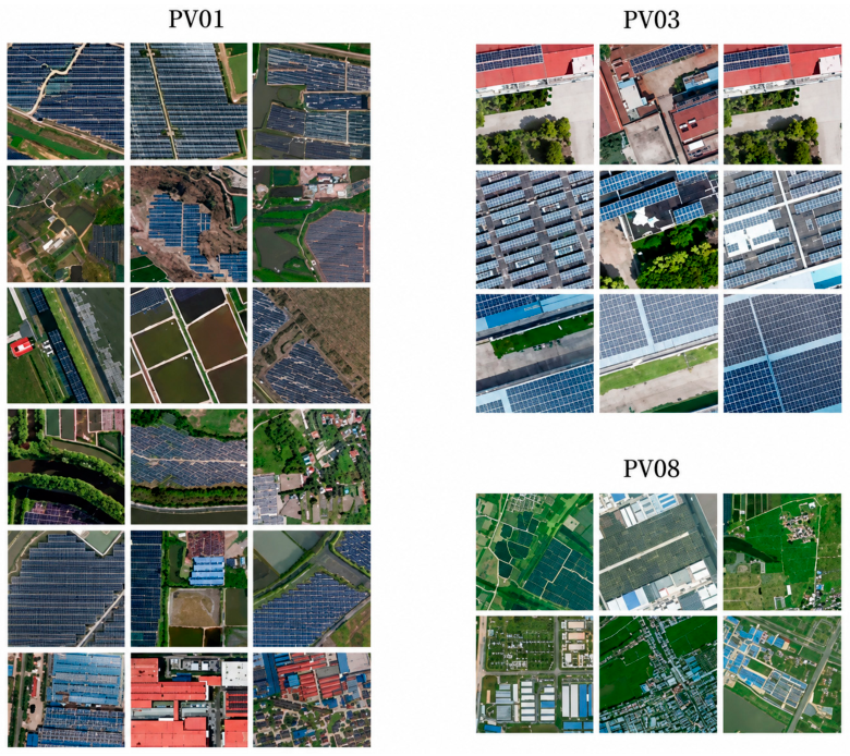
The images were divided into three GSD tiers according to platform and nominal GSD. PV08 contains satellite images with a nominal GSD of 0.8 m. These images provide wide coverage but show strong spectral mixing and blurred panel boundaries. PV03 contains fixed-wing aerial photogrammetry images with a nominal GSD of 0.3 m. This tier provides regional coverage and preserves array topology more clearly. PV01 contains multi-rotor UAV images with a nominal GSD of 0.1 m. It resolves fine cell gaps, frames, and local reflections.

Table 2. Summary of the three image-acquisition tiers.

Dataset Tier	Observation Platform	Nominal GSD	Main Image Characteristics
PV08	Gaofen-2/Beijing-2 satellite	0.8 m	Wide-area coverage; strong spectral mixing; blurred panel boundaries
PV03	Fixed-wing aerial photogrammetry	0.3 m	Regional coverage; clear array topology; varied installation azimuths
PV01	Multi-rotor UAV	0.1 m	Fine structural detail; visible cell gaps and metal frames

summarizes the three acquisition tiers.

PV08 primarily covers large industrial zones, where arrays are commonly installed on corrugated steel roofs amid bright roofs, shadows, roads, and storage areas. PV03 covers smaller, more irregular rural and suburban rooftop systems. PV01 was acquired from UAV flights at 50–120 m above ground. It contains stronger local texture and finer boundaries, together with glare, water reflections, and occlusions. 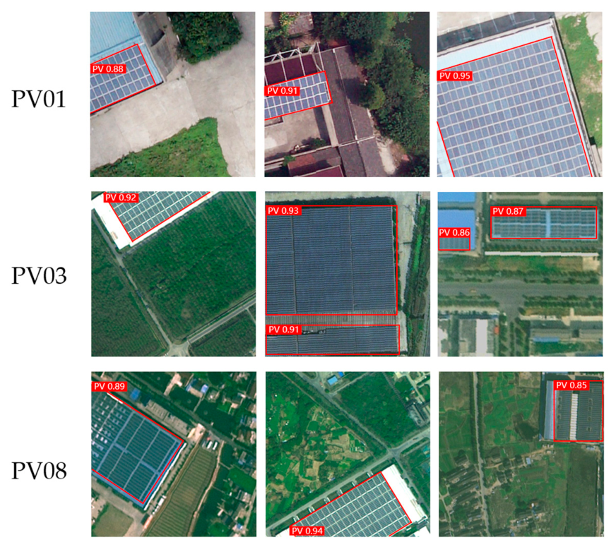Figure 3 shows representative examples from the three tiers.

All visible PV panel areas were annotated with polygon masks. Support structures, shadows, non-PV roof materials, and adjacent ground were excluded to keep mask definitions consistent across GSD tiers. For detection, each polygon was converted to its minimum-area rotated rectangle. Its axis-aligned enclosure was used as the corresponding horizontal bounding box.

Annotation quality was assessed in three steps. First, all labels were created with a vector annotation tool. Second, 300 complex image patches were independently reviewed by two researchers familiar with PV remote-sensing annotation. Third, agreement for pixel-level binary PV/non-PV labels was measured using Cohen’s kappa:

$$\kappa ={\displaystyle \frac{p_o-p_e}{1-p_e}},$$

(1)

where $p_o$ is the observed agreement and $p_e$ is the agreement expected by chance. The measured kappa value was 0.80, indicating good annotation consistency. Ambiguous cases were resolved by consensus, especially in PV08 images containing bright roof coatings.

During training, random cropping, scaling, flipping, and rotation were applied as geometric augmentations. Cropping, flipping, and rotation do not change the physical ground resolution and therefore retain the original GSD. For random scaling, let $a$ denote the ratio of the augmented image size to the original image size. The effective GSD provided to the Physical GSD Embedding was updated as:

$$s_{\mathrm{a}\mathrm{u}\mathrm{g}}=s/a,$$

(2)

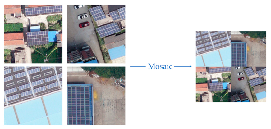
where $s$ is the nominal GSD before augmentation. Mosaic augmentation was restricted to patches from the same GSD tier. The component patches were assembled without independent scale factors, and any subsequent global scaling of the mosaic used a shared factor $a$, with its effective GSD updated accordingly.

The same augmentation policy was applied to CRFA-PVNet and all baseline models to maintain consistent training conditions. The mosaic augmentation process is illustrated in Figure 4.

3.2. Spatial Autocorrelation-Based Data Partitioning

Random-patch partitioning can introduce spatial information leakage, so the dataset was divided with a spatially disjoint protocol. Moran’s I was used here as a global indicator of spatial autocorrelation [41]. Its standard spatial interpretation follows the framework of Cliff and Ord [42]. In our setting, it was used as a diagnostic of background dependence before defining the buffer distance. The first step was therefore to compute Global Moran’s I over patch-level background feature values:

$$I={\displaystyle \frac{N}{S_0}}{\displaystyle \frac{{\sum }_{i=1}^N{\sum }_{j=1}^N{w}_{ij}(x_i-\overline{x})(x_j-\overline{x})}{{\sum }_{i=1}^N(x_i-\overline{x}{)}^2}},$$

(3)

where N is the number of patches, $x_i$ and $x_j$ are background feature values at locations i and j, $\overline{x}$ is the global mean, $w_{ij}$ is the spatial weight between two patch centers, and $S_0={\sum }_i{\sum }_j{w}_{ij}$. The background feature value was computed from spectral and texture descriptors after excluding annotated PV pixels. This choice reduces the influence of target density and focuses the statistic on environmental similarity.

Geostatistical analysis of the original image patches yielded a Global Moran’s I of 0.68, indicating strong positive spatial autocorrelation. The semivariogram was then used to characterize how this dependence decreased with increasing separation distance. The practical buffer distance was selected by jointly considering the semivariogram trend and the sample-size requirements of the data partition.

Moran’s I indicates the presence of spatial dependence but does not directly determine a practical separation distance. We therefore computed an empirical semivariogram:

$$\gamma (h)={\displaystyle \frac{1}{2N(h)}}{\sum }_{i=1}^{N(h)}[Z(s_i)-Z(s_i+h){]}^2,$$

(4)

where $N(h)$ is the number of paired samples separated by lag h, and $Z(s_i)$ is the local background descriptor at location $s_i$. The empirical semivariogram was fitted using a spherical model. The fitted curve showed a rapid increase in semivariance at short separation distances, followed by a progressively slower increase beyond approximately 5 km. This pattern indicates that the marginal reduction in spatial dependence became smaller after this distance, although the fitted sill was reached at a larger separation. Considering this transition, the preservation of municipal and scene continuity, and the need to maintain sufficient samples in the training, validation, and test subsets, 5 km was selected as a practical minimum buffer distance.

The dataset was partitioned by geographic location rather than by random-patch sampling. Samples were first grouped according to the center coordinates of image patches. These spatial groups were then assigned to the training, validation, and test subsets. A minimum spatial separation of 5 km was maintained between the training, validation, and testing sectors. City boundaries were also used as an auxiliary constraint to avoid assigning continuous urban or rural scenes to different subsets. This protocol reduced the risk that geographically adjacent patches with similar backgrounds appeared in different data subsets.

Under this protocol, the patch allocation ratio was approximately 60% training, 10% validation, and 30% testing. PV08 included 12,400 patches and 45,210 annotated PV regions, of which 7412 patches were used for training, 1253 for validation, and 3735 for testing. PV03 included 8200 patches and 28,150 annotated PV regions, with 4904, 831, and 2465 patches assigned to training, validation, and testing, respectively. PV01 included 6500 patches and 18,920 annotated PV regions, with 3892, 658, and 1950 patches assigned to the three subsets, respectively.

Figure 5 summarizes the dataset allocation and spatial validation protocol. It reports the train-validation-test split for PV08, PV03, and PV01 and illustrates the 5 km buffer used for spatial separation. It also shows the Moran’s I and semivariogram diagnostics used to determine the buffer distance.

3.3. Physical Receptive Field (PRF)

The three PV image tiers differ in GSD, so the same pixel-level receptive field corresponds to different ground spans in PV08, PV03, and PV01. We therefore define the physical receptive field as a first-order estimate of the ground span associated with a convolutional feature. This approximation assumes orthorectified images, approximately isotropic GSD, and locally constant ground resolution.

Let $R_l$ be the receptive field size, in pixels, of a feature unit at layer l. Let s be the nominal GSD of the input image in meters per pixel. The linear physical receptive field is defined as:

$$\Phi (l,s)=R_l\times s.$$

(5)

Here, the physical receptive field is a first-order estimate of the ground span associated with the theoretical receptive field. It is not the effective receptive field, which can be smaller and data dependent.

The corresponding physical area is:

$$A_{\mathrm{P}\mathrm{R}\mathrm{F}}(l,s)={\left(R_{l}s\right)}^2$$

(6)

This identifies one geometric source of cross-resolution mismatch in PV extraction. If $R_l$ is fixed and s increases from 0.1 m to 0.8 m, the linear ground span grows by a factor of 8. The physical area grows by a factor of 64. A feature unit that observes local cell texture in UAV images may observe several arrays and background objects in satellite images. The hidden representation may therefore mix different types of visual evidence across GSD tiers.

To distinguish physical scale separation from model-dependent error, we define the cross-resolution physical-support gap between two GSD conditions at the same layer as:

$$D_{\mathrm{P}\mathrm{S}}(s_i,s_j)=\left|{\mathrm{l}\mathrm{o}\mathrm{g}}_2{\displaystyle \frac{{\Phi }_l(s_i)}{{\Phi }_l(s_j)}}\right|=\left|{\mathrm{l}\mathrm{o}\mathrm{g}}_2{\displaystyle \frac{s_i}{s_j}}\right|$$

(7)

This dimensionless quantity, which describes geometric scale separation, equals zero for identical GSDs and increases with their relative separation.

For co-registered observations of the same ground scene at two GSDs, the fusion features at layer l are spatially aligned to a common ground grid, and the error is defined as:

$$E_{\mathrm{C}\mathrm{R}}^{\left(l\right)}(s_i,s_j)={\displaystyle \frac{{‖{\tilde{F}}_l^{\left(s_i\right)}−{\tilde{F}}_l^{\left(s_j\right)}‖}_F}{{‖{\tilde{F}}_l^{\left(s_i\right)}‖}_F+{‖{\tilde{F}}_l^{\left(s_j\right)}‖}_F+\epsilon }}$$

(8)

Here, the tilde denotes spatial alignment to the common ground grid, the Frobenius norm measures the discrepancy between the aligned feature tensors, and epsilon prevents division by zero. The normalization makes the error symmetric, dimensionless, and bounded between 0 and 1. A larger physical-support gap exposes a fixed pixel-domain operator to less equivalent ground evidence. This motivates the empirically testable hypothesis that representation error tends to increase with the gap and that GSD conditioning can reduce it at a given gap.

The diagnostic is evaluated at the principal multi-scale fusion level where CRFA operates. Features from each GSD condition are bilinearly aligned to the common 0.1 m ground grid, the 0.1 m observation of the same scene is used as the reference, and the scene-wise normalized errors are averaged over the held-out set.

To reduce this mismatch, we define a target physical span ${\Phi }^{\ast }$. The ideal pixel receptive field should vary with GSD:

$$\Phi (l,s)=R_l(s)\times s\equiv {\Phi }^{\ast }.$$

(9)

Solving for the adaptive pixel receptive field gives:

$$R_l(s)={\displaystyle \frac{{\Phi }^{\ast }}{s}}.$$

(10)

This equation guides the design of the feature alignment module. The network should still learn adaptive sampling and reassembly. However, conditioning on physical resolution provides the model with an explicit cue for adapting feature aggregation across the PV08, PV03, and PV01 images.

Figure 6 illustrates physical receptive-field scaling. With a fixed pixel receptive field, linear ground span grows in proportion to GSD, whereas physical area grows quadratically. Moving from the 0.1 m UAV tier to the 0.8 m satellite tier therefore expands linear span by a factor of 8 and area by a factor of 64. A fixed target ground span requires a smaller pixel receptive field as GSD increases.

This formulation links physical sampling scale to feature aggregation and motivates the CRFA module described next.

3.4. Physically Guided Cross-Resolution Feature Alignment

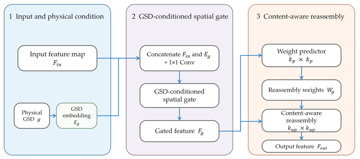
The CRFA module is designed to align feature fusion with physical image scale. Given an input feature map $F_{in}\in R^{C\times H\times W}$ and the image GSD s, the module maps it to a scale-modulated feature. During training, s denotes the effective GSD after geometric scaling. The output is denoted by $F_{out}$. Its forward process has three steps. It first converts the scalar GSD into a richer embedding. It then uses this embedding to generate a spatial gate. Finally, it predicts content-aware reassembly kernels from the gated features. This design keeps the module lightweight while making the feature fusion stage aware of the physical scale represented by each pixel.

The first step is Physical GSD Embedding. Feeding one scalar directly into a deep network provides limited representational capacity. We therefore use a sinusoidal embedding inspired by positional and Fourier feature encodings:

$$PE(s,2i)=\mathrm{s}\mathrm{i}\mathrm{n}\left({\displaystyle \frac{s}{{10000}^{2i/C}}}\right),PE(s,2i+1)=\mathrm{c}\mathrm{o}\mathrm{s}\left({\displaystyle \frac{s}{{10000}^{2i/C}}}\right),$$

(11)

where i indexes the embedding frequencies and C is the target channel width. The embedded vector is passed through a small multilayer perceptron to obtain:

$$E_P(s)\in R^{C\times 1\times 1}.$$

(12)

This representation gives the network a richer description of the resolution, and it keeps the module lightweight because the embedding is computed once per image or patch.

The second step is adaptive spatial gating. To make the physical-scale condition responsive to local image content, the embedding is broadcast along the spatial dimensions and multiplied with the input feature map. A 1 × 1 projection and sigmoid activation then generate a spatial gate:

$$F_{gate}=\sigma (W_g·[F_{in}\otimes E_P(s)])\in R^{1\times H\times W},$$

(13)

where the broadcast product combines the GSD-conditioned descriptor with the input feature map, and $W_g$ is a learnable projection. The gated feature map is:

$$F_{mod}=F_{in}\odot F_{gate}.$$

(14)

The gate changes spatial emphasis according to the input resolution. In high-resolution UAV images, it can retain fine boundary and cell-texture responses. In lower-resolution satellite images, it can suppress noisy responses from roof texture, soil, and metal supports. Because the gate is learned, it adapts to local image content while remaining conditioned on GSD.

The third step is GSD-conditioned content-aware feature reassembly. Spatial gating can rescale existing responses, whereas local feature aggregation is determined by the weights assigned within each sampling neighborhood. Inspired by CARAFE [15], a lightweight predictor $\psi$ therefore generates a normalized local reassembly kernel at each output position $x^{\prime }$ from the GSD-conditioned features:

$${W^{\prime }}_{x^{\prime }}=softmax\left[\psi \left(F_{\mathrm{m}\mathrm{o}\mathrm{d}}(x^{\prime })\right)\right]\in {\mathbb{R}}^{k_{\mathrm{u}\mathrm{p}}\times k_{\mathrm{u}\mathrm{p}}}$$

(15)

where $k_{up}$ is the reassembly kernel size. The normalized kernel is then applied to the corresponding input neighborhood:

$$F_{\mathrm{o}\mathrm{u}\mathrm{t}}(x^{\prime })={\sum }_{n\in \mathcal{N}(x^{\prime },k_{\mathrm{u}\mathrm{p}})}{W^{\prime }}_{x^{\prime }}(n)F_{\mathrm{i}\mathrm{n}}(n)$$

(16)

In Equations (13)–(16), the broadcast product combines the GSD descriptor with the input feature map. And the element-wise product applies the spatial gate. The predictor psi maps the modulated feature at x′ to a $k_{up}$ by $k_{u\mathrm{p}}$ kernel. Softmax normalizes the kernel weights over the neighborhood N(x′, $k_{up}$) before reassembly.

Standard content-aware reassembly predicts image-dependent kernels from image features alone, which can be written as $K(X)$. In CRFA, the kernel predictor receives features already modulated by effective GSD, so the local weights become $K(X,s_{\mathrm{e}\mathrm{f}\mathrm{f}})$. The resulting operation is both content-aware and conditioned on a physical scale. Feature aggregation accounts for the ground scale represented by each pixel as a result.

In implementation, CRFA is inserted into the feature fusion stage, where multi-scale features are merged and upsampled. Cross-resolution misalignment is most visible at this stage. The module adds few parameters relative to the backbone and prediction heads. The alignment channel width C and reassembly kernel size $k_{up}$ are evaluated in Section 4.2.

Figure 7 shows the internal computation of CRFA. Physical GSD Embedding first projects the scalar GSD into a resolution descriptor. The descriptor is broadcast and combined with the input feature map to produce a GSD-conditioned spatial gate. A lightweight predictor then estimates local reassembly weights from the gated features, and content-aware reassembly produces the output. The schematic uses $k_p$ for the predictor context window and $k_{up}$ for the output reassembly-kernel size.

3.5. Proposal-Guided Local Mask Refinement Pipeline

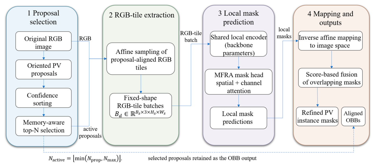
The proposal-guided local mask refinement pipeline reduces the cost of full-frame mask prediction while preserving local boundary information. A lightweight proposal branch predicts oriented PV candidates. The local mask refinement branch predicts masks only within proposal-aligned RGB tiles sampled from the input image. Fine boundary parsing is therefore restricted to selected proposal regions instead of being applied to large background areas.

As shown in Figure 8, the proposal branch predicts oriented PV boxes, ranks them by confidence, and retains a memory-aware top-N subset. Each selected proposal guides affine sampling of a proposal-aligned RGB tile from the original image, and the sampled tiles are assembled into fixed-size batches. A shared local encoder and the Multilayer Feature Reconstruction Attention (MFRA) mask head predict a local mask for each tile. The local masks are mapped back to the image coordinate system and merged using score-based fusion, while the selected proposals are retained as the aligned OBB outputs.

CRFA improves cross-resolution representation but does not itself remove the cost of full-frame mask prediction. The Proposal-Guided Local Mask Refinement pipeline separates proposal generation from boundary refinement. The proposal branch filters most background pixels, and the local mask refinement branch refines masks only in selected regions. This allocation retains fine parsing where it is needed without applying dense segmentation to an empty background.

The proposal generation branch scans the input image and predicts oriented PV candidates. The backbone uses Partial Convolution (PConv) blocks to reduce computation. For an input tensor $F_{in}$, only the fraction $c_p=rC$ of the channels is processed by spatial convolution:

$$F_{out}=[{\mathrm{Conv}}_{k\times k}(F_{in}[:,:c_p,:,:]);F_{in}[:,c_p:,:,:\left]\right].$$

(17)

In this work, $r=1/4$. The spatial convolution is therefore applied to one quarter of the channels. This reduces the multiply-accumulate operations of the spatial part and lowers memory access. A channel mixing layer is used after the partial operation to maintain information exchange.

The detection head predicts oriented bounding boxes:

$$b_i=(x_{c,i},y_{c,i},w_i,h_i,{\theta }_i),$$

(18)

where ($x_c$, $y_c$) is the box center, $w$ and $h$ are its long-edge width and short-edge height, and $\theta$ is the orientation angle. We use the long-edge convention $w\ge h$ and $\theta$ in [−π/2, π/2). This representation avoids equivalent width-height swaps.

The oriented-box regression objective combines an SIoU-inspired geometric term [48] with explicit periodic orientation supervision. For a predicted box b and ground-truth box b*, the geometric term is:

$$L_{\mathrm{g}\mathrm{e}\mathrm{o}\mathrm{m}}=1-{IoU}_{\mathrm{r}\mathrm{o}\mathrm{t}}(b,b^{\ast })+{\displaystyle \frac{\Delta +\Omega }{2}}$$

(19)

where ${IoU}_{\mathrm{r}\mathrm{o}\mathrm{t}}$ is rotated intersection over union, and $\Delta$ and $\Omega$ are the SIoU distance and shape costs, respectively. Orientation is supervised by the pi-periodic term $L_{ori}=1-cos[2(\theta -{\theta }^{\ast })]$. The complete OBB regression loss is:

$$L_{\mathrm{O}\mathrm{B}\mathrm{B}}=L_{\mathrm{g}\mathrm{e}\mathrm{o}\mathrm{m}}+{\lambda }_{\theta }\left\{1−\mathrm{c}\mathrm{o}\mathrm{s}\left[2(\theta -{\theta }^{\ast })\right]\right\}$$

(20)

In Equations (19) and (20), ${\lambda }_{\theta }$ controls the orientation term. The doubled angular difference makes the loss invariant to a 180-degree representation of the same rectangle. This formulation supervises overlap, center and shape consistency, and the OBB angle.

The combined objective reduces center and shape mismatch while directly constraining box orientation. This is important for the long, narrow, and frequently tilted PV arrays used to guide local mask refinement.

After oriented proposal generation, candidate boxes are sorted by confidence. Sending every candidate to local mask refinement can cause unstable memory use. We therefore define a memory-aware upper bound:

$$N_{max}=⌊{\displaystyle \frac{\alpha M_{\mathrm{a}\mathrm{v}\mathrm{a}\mathrm{i}\mathrm{l}}}{M_{\mathrm{s}\mathrm{e}\mathrm{g}}}}⌋$$

(21)

where $M_{\mathrm{a}\mathrm{v}\mathrm{a}\mathrm{i}\mathrm{l}}$ is the device memory remaining after model parameters, fixed feature tensors, and runtime buffers are allocated. $M_{\mathrm{s}\mathrm{e}\mathrm{g}}$ is the estimated cost of one segmentation tile, and alpha is a safety coefficient. In the experiments, alpha = 0.85. Let $N_{\mathrm{p}\mathrm{r}\mathrm{o}\mathrm{p}}$ denote the number of proposals remaining after confidence-based sorting and filtering. The number of active proposals is

$$N_{active}=\lfloor min(N_{prop},N_{max})\rfloor .$$

(22)

Only the top $N_{active}$ proposals are sent to the local mask refinement branch. The floor operator in Equation (22) ensures that the selected proposal count is an integer and does not exceed the available memory budget.

For each active proposal, the oriented box is mapped from the input-image coordinate system to a normalized local RGB tile. The affine matrix is:

$$M_{affine,i}=\left[\begin{array}{ccc}{\displaystyle \frac{w_i}{2}}\mathrm{c}\mathrm{o}\mathrm{s}{\theta }_i& -{\displaystyle \frac{h_i}{2}}\mathrm{s}\mathrm{i}\mathrm{n}{\theta }_i& x_{c,i}\\ {\displaystyle \frac{w_i}{2}}\mathrm{s}\mathrm{i}\mathrm{n}{\theta }_i& {\displaystyle \frac{h_i}{2}}\mathrm{c}\mathrm{o}\mathrm{s}{\theta }_i& y_{c,i}\end{array}\right].$$

(23)

Given normalized coordinates $(u,v)\in [-\mathrm{1,1}]\times [-\mathrm{1,1}]$, the source image coordinates are:

$$\left[\begin{array}{c}{x}_i(u,v)\\ y_i(u,v)\end{array}\right]=M_{affine,i}\left[\begin{array}{c}u\\ v\\ 1\end{array}\right].$$

(24)

Equivalently,

$$x_i(u,v)=u{\displaystyle \frac{w_i}{2}}\mathrm{c}\mathrm{o}\mathrm{s}{\theta }_i-v{\displaystyle \frac{h_i}{2}}\mathrm{s}\mathrm{i}\mathrm{n}{\theta }_i+x_{c,i},$$

(25)

$$y_i(u,v)=u{\displaystyle \frac{w_i}{2}}\mathrm{s}\mathrm{i}\mathrm{n}{\theta }_i+v{\displaystyle \frac{h_i}{2}}\mathrm{c}\mathrm{o}\mathrm{s}{\theta }_i+y_{c,i}.$$

(26)

The local RGB tile $T_i$ is sampled from the input image by bilinear interpolation:

$$T_i(u,v)={\sum }_{x^{\prime }=0}^{W_{\mathrm{r}\mathrm{a}\mathrm{w}}-1}{\sum }_{y^{\prime }=0}^{H_{\mathrm{r}\mathrm{a}\mathrm{w}}-1}I(x^{\prime },y^{\prime })max(\mathrm{0,1}-|x_i(u,v)-x^{\prime }|)max(\mathrm{0,1}-|y_i(u,v)-y^{\prime }|)$$

(27)

This mapping projects the oriented proposal onto a regular local grid without a hand-crafted crop heuristic, and the same transformation projects the refined local mask back to the original image.

The local mask refinement branch refines the PV mask inside each active tile. To reduce cost, standard dilated convolutions are replaced with asymmetric depthwise operations, such as $1\times d$ and $d\times 1$ filters. A Multilayer Feature Reconstruction Attention (MFRA) head is used before mask prediction. It computes spatial and channel attention:

$$A_s=\sigma ({\mathrm{Conv}}_{1\times 1}([\mathrm{AvgPool}(F);\mathrm{MaxPool}(F)])),$$

(28)

$$A_c=\sigma (\mathrm{MLP}(\mathrm{AvgPool}(F))+\mathrm{MLP}(\mathrm{MaxPool}(F))).$$

(29)

The final feature is refined by both attention maps. This helps sharpen PV boundaries in the presence of glare, roof edges, and mixed pixels. The local tiles are packed into fixed-size batches:

$$B_d=[B1,B2,\dots ,B_{BS}]\in {\mathbb{R}}^{B_s\times 3\times H_s\times W_s}$$

(30)

Here, ${\mathrm{B}}_k\in {\mathbb{R}}^{3\times H_s\times W_s}$ denotes the proposal-aligned RGB tile at the $k$-th batch position. $B_s$ is the fixed local batch size, $H_s$ and $W_s$ denote the fixed height and width of each sampled RGB tile, respectively. The channel dimension is three because each tile is sampled from the input RGB image. Empty slots are padded with zeros to keep tensor dimensions fixed, avoid repeated dynamic-shape compilation, and limit memory variation during edge inference.

4. Experiments and Analysis

The experiments evaluate detection and segmentation accuracy, module contributions, spatial reliability, cross-dataset transfer, and edge-side efficiency. PV08, PV03, and PV01 represent satellite, aerial, and UAV images with different GSDs [47]. CRFA-PVNet is compared with YOLOv9-C [29], YOLOv10-B [30], RT-DETR-L [31], Oriented R-CNN [25], S²A-Net [27], Rotated RTMDet-M [28], and Mask2Former [32]. The ablation experiments examine Physical GSD Embedding, spatial gating, proposal-guided local mask refinement pipeline, and MFRA.

All models were trained under one common protocol. A single unified model was jointly trained on the pooled PV08, PV03, and PV01 training subsets. Samples from the three tiers were globally shuffled, and each mini-batch was drawn from this pooled training set. During training, the effective GSD associated with each augmented image was passed to the Physical GSD Embedding branch. For samples without geometric scaling, the effective GSD was equal to the nominal tier GSD. The three CRFA-PVNet rows in

Table 3. Quantitative comparison across the three GSD tiers. N/A = Not Applicable, indicating that the corresponding metric cannot be calculated for this case.

Model	Tier	Precision	Recall	F1-Score	OBB mAP50	Mask IoU
YOLOv9-C [29]	PV08	0.762	0.695	0.727	0.741	N/A
YOLOv9-C [29]	PV03	0.841	0.812	0.826	0.835	N/A
YOLOv9-C [29]	PV01	0.884	0.863	0.873	0.879	N/A
YOLOv10-B [30]	PV08	0.751	0.684	0.716	0.735	N/A
YOLOv10-B [30]	PV03	0.839	0.798	0.818	0.829	N/A
YOLOv10-B [30]	PV01	0.891	0.854	0.872	0.882	N/A
RT-DETR-L [31]	PV08	0.784	0.702	0.741	0.759	N/A
RT-DETR-L [31]	PV03	0.856	0.823	0.839	0.851	N/A
RT-DETR-L [31]	PV01	0.902	0.871	0.886	0.895	N/A
Oriented R-CNN [25]	PV08	0.794	0.713	0.751	0.773	N/A
Oriented R-CNN [25]	PV03	0.873	0.845	0.859	0.868	N/A
Oriented R-CNN [25]	PV01	0.912	0.891	0.901	0.914	N/A
S2A-Net [27]	PV08	0.809	0.738	0.772	0.792	N/A
S2A-Net [27]	PV03	0.881	0.849	0.865	0.879	N/A
S2A-Net [27]	PV01	0.919	0.897	0.908	0.921	N/A
Rotated RTMDet-M [28]	PV08	0.824	0.756	0.789	0.807	N/A
Rotated RTMDet-M [28]	PV03	0.894	0.858	0.876	0.889	N/A
Rotated RTMDet-M [28]	PV01	0.929	0.906	0.917	0.930	N/A
Mask2Former [32]	PV08	0.731	0.652	0.689	0.692	0.612
Mask2Former [32]	PV03	0.824	0.791	0.807	0.784	0.734
Mask2Former [32]	PV01	0.895	0.874	0.884	0.851	0.821
Ours	PV08	0.864	0.811	0.837	0.849	0.764
Ours	PV03	0.915	0.887	0.901	0.912	0.843
Ours	PV01	0.948	0.932	0.940	0.945	0.891

were evaluated using the same learned parameter set. S²A-Net and Rotated RTMDet-M were evaluated on the same spatially disjoint partitions, with the same input size, OBB annotations, and evaluation protocol. Training was conducted on an NVIDIA RTX 3090 GPU. The latency, peak device memory, and FPS values in

Table 4. Ablation results under the spatially disjoint protocol.

Configuration	PGE	Spatial Gating	Proposal-Guided Ref.	MFRA	OBB mAP50 (PV08)	Mask IoU (PV01)	Latency (ms)	Peak Device Memory (GB)	FPS
1 (Baseline)	No	No	No	No	0.745	0.812	238.1	6.42	4.2
2	Yes	No	No	No	0.782	0.824	243.9	6.45	4.1
3	Yes	Yes	No	No	0.814	0.838	256.4	6.48	3.9
4 (Framework shift)	Yes	Yes	Yes	No	0.816	0.841	31.8	3.95	31.4
5 (Full model)	Yes	Yes	Yes	Yes	0.849	0.891	35.2	4.21	28.4

were measured using the native PyTorch 1.12 FP32 implementation on an NVIDIA Jetson TX2 after warm-up under a unified single-frame inference setting. Runtime-level effects of TensorRT 1.12 FP32 and FP16 deployment are evaluated separately in Section 4.5. To assess training stochasticity, CRFA-PVNet, Rotated RTMDet-M, and Mask2Former were each independently trained with three random seeds. Each CRFA-PVNet run used one jointly trained parameter set for evaluation across the PV08, PV03, and PV01 tiers. Results are reported as the mean ± sample standard deviation over the three runs; macro metrics were calculated as the unweighted mean across the three tiers within each run, and two-sided 95% confidence intervals summarize seed-matched differences from the corresponding baseline.

Detection performance was evaluated using precision, recall, F1-score, and oriented-bounding-box mean average precision at an IoU threshold of 0.5 (OBB mAP50). Precision–recall measures are standard in object-detection benchmarks [49], and later reviews describe their false-alarm and missed-detection trade-offs [50]. For a common geometric evaluation, every ground-truth polygon or mask was converted to its minimum-area rotated rectangle. Native OBB predictions were evaluated directly. Connected mask components were converted to minimum-area rotated rectangles, whereas a horizontal Bounding Box prediction was represented as the special OBB case $\theta =0^{\circ }$. All methods were compared with the same OBB ground truth using rotated IoU at a threshold of 0.5. Mask IoU was reported only for methods that produced pixel-level masks. The converted OBB scores should be interpreted under this common protocol rather than as each model’s native benchmark metric.

4.1. Cross-Resolution Performance Evaluation

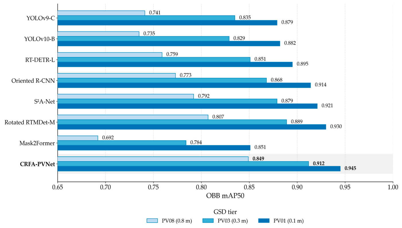
To evaluate the cross-resolution performance of CRFA-PVNet, we compared it with representative detection and segmentation models on PV08, PV03, and PV01. These datasets represent satellite, aerial, and UAV imagery, respectively. Table 3 reports the quantitative results for oriented detection and instance segmentation across the three tiers. Figure 9 summarizes the corresponding OBB mAP50 results.

YOLOv9-C [29], YOLOv10-B [30], and RT-DETR-L [31] represent general-purpose object detectors. Oriented R-CNN [25], S²A-Net [27], and Rotated RTMDet-M [28] provide dedicated oriented-detection baselines. Mask2Former [32] serves as the mask-capable segmentation baseline. CRFA-PVNet is evaluated in both tasks because it produces OBBs and proposal-guided instance masks within one jointly trained framework. PV arrays exhibit substantial changes in apparent size, edge clarity, and background context across the three tiers. The tier-wise results show how these changes affect localization and segmentation performance. They also assess whether CRFA-PVNet maintains consistent cross-resolution performance.

Figure 9 summarizes the OBB mAP50 values in Table 3. S²A-Net and Rotated RTMDet-M outperform Oriented R-CNN across the three GSD tiers. Rotated RTMDet-M is the strongest dedicated oriented-detection baseline, reaching 0.807, 0.889, and 0.930 on PV08, PV03, and PV01 respectively.

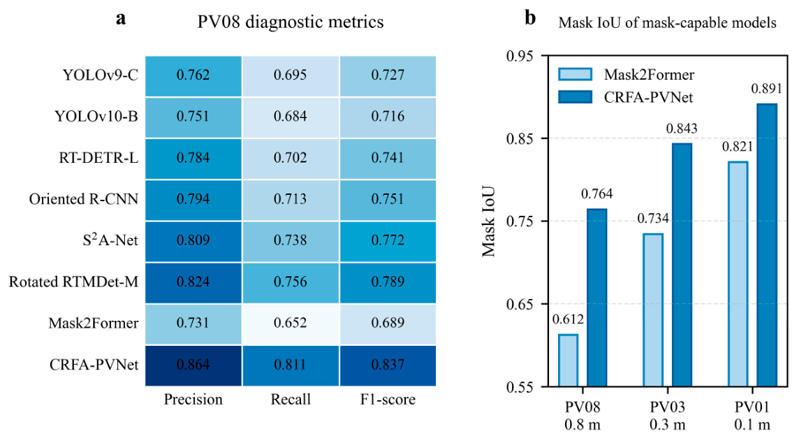
CRFA-PVNet achieves the highest OBB mAP50 on all three tiers. Relative to Rotated RTMDet-M, it improves OBB mAP50 by 0.042, 0.023, and 0.015 on PV08, PV03, and PV01 respectively. The largest margin occurs on PV08, where panel boundaries are blurred and background mixing is stronger. For the mask-capable comparison, mask IoU increases from 0.612 for Mask2Former to 0.764 for CRFA-PVNet on PV08.

On PV03, the proposed model reaches 0.912 OBB mAP50 and 0.843 mask IoU. The gain is smaller than on PV08 but still clear, because aerial images preserve more PV geometry and the baselines already perform well. CRFA nonetheless helps by aligning features across local scale changes and by reducing background interference from roof structures.

On PV01, the proposed model reaches 0.945 OBB mAP50 and 0.891 mask IoU. The high-resolution UAV tier contains fine cell patterns and sharper edges. Here, the main benefit comes from the local mask refinement branch and the MFRA head. Local boundary refinement improves mask quality, while oriented proposals reduce unnecessary background inside the segmentation crop.

Table 3 reports PV08, PV03, and PV01 results under the common OBB protocol. Precision, recall, and F1-score describe false alarms and missed detections, while OBB mAP50 measures rotated localization at an IoU threshold of 0.5. The three GSD tier results use one jointly trained parameter set.

Figure 10 visualizes the main benchmark diagnostics. Detection metrics and mask-quality results are presented separately to distinguish localization performance from pixel-level segmentation quality. The PV08 panel reports precision, recall, and F1-score under the adopted inference setting. The mask-quality panel compares mask IoU across the three PV tiers for models that produce pixel-level masks.

The comparison also shows the limitation of detection-only models for joint PV detection and segmentation. YOLOv9, YOLOv10, RT-DETR, Oriented R-CNN, S²A-Net, and Rotated RTMDet-M localize arrays but do not provide the fine masks needed for area estimation or panel-level inspection. Mask2Former produces masks but applies dense prediction to the full frame and performs less robustly on the coarse PV08 tier. The proposed pipeline instead combines oriented localization with mask refinement in selected regions.

To further illustrate these differences, Figure 11 compares representative predictions from coarse satellite images, aerial images, and UAV images. The qualitative results show that the proposed model performs with high detection accuracy.

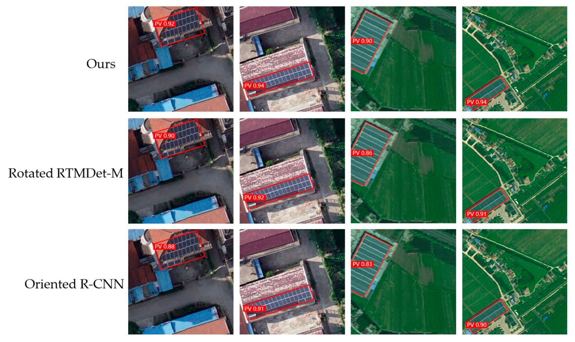
Figure 12 compares representative predictions from CRFA-PVNet, Rotated RTMDet-M, and Oriented R-CNN under the same evaluation protocol. All three methods localize the principal PV arrays, while CRFA-PVNet gives the highest confidence score in each displayed case.

Overall, the quantitative comparison shows that CRFA-PVNet maintains stable performance across different GSD tiers, with the most evident gain appearing on the coarse PV08 satellite tier.

4.2. Ablation Insights and Parameter Sensitivity Analysis

This subsection evaluates the contribution of each CRFA-PVNet component and the sensitivity of the main hyperparameters. The ablation includes Physical GSD Embedding, spatial gating, proposal-guided local mask refinement pipeline, and MFRA. The sensitivity analysis examines the embedding channel width C and the reassembly kernel size. Table 4 reports the results under the spatially disjoint protocol.

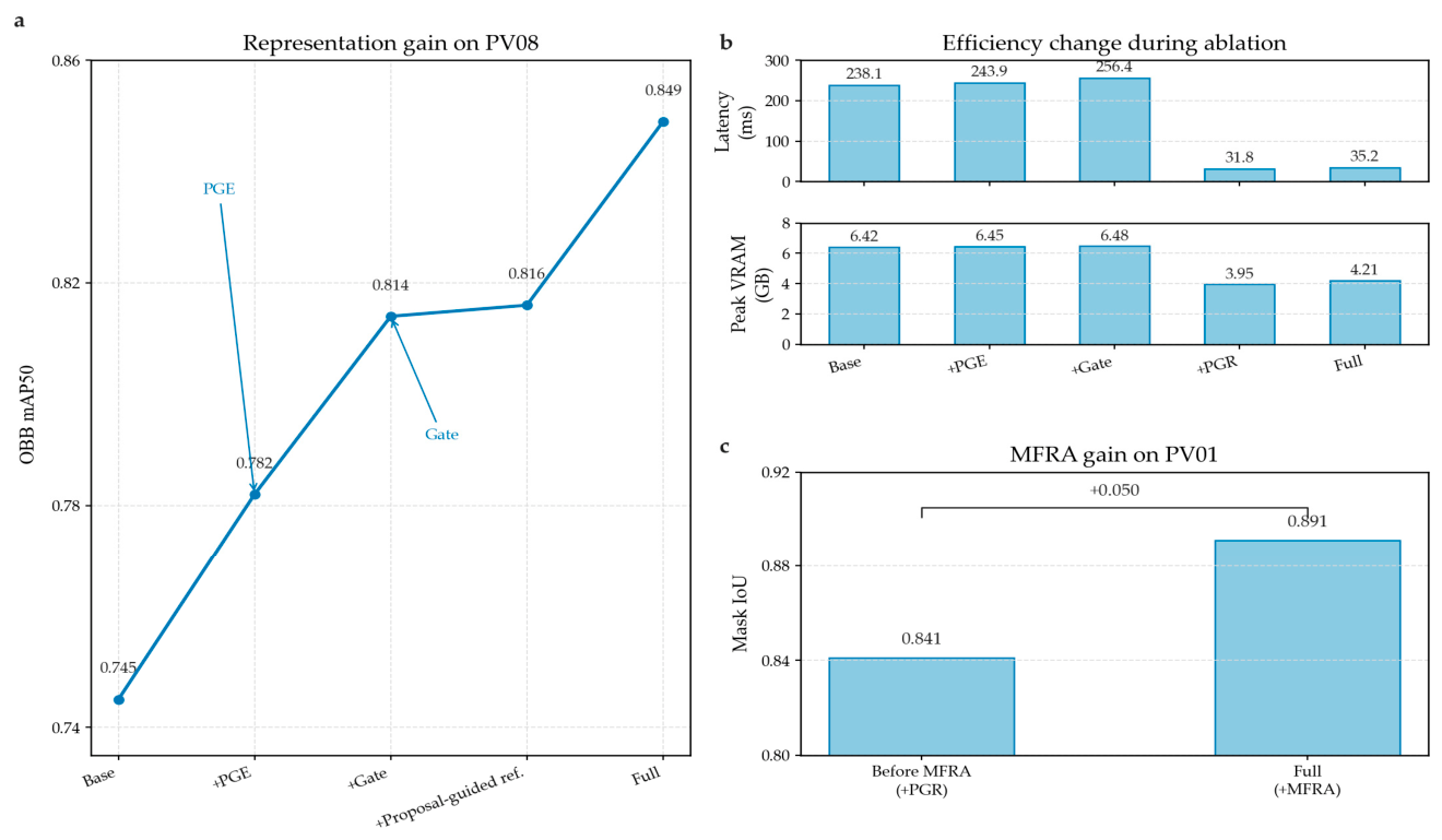
Figure 13 summarizes the component effects. Figure 13a shows PV08 OBB mAP50 as representation modules are added. Figure 13b reports latency and peak memory after the proposal-guided local mask refinement pipeline is introduced. Figure 13c shows the PV01 mask IoU gain from MFRA.

Adding PGE increases PV08 OBB mAP50 from 0.745 to 0.782. This suggests that an appropriately encoded GSD scalar improves representation. The small latency change indicates that the gain is primarily representational rather than computational.

Adding spatial gating further raises PV08 OBB mAP50 to 0.814. GSD embedding alone is not sufficient; the resolution cue must influence spatial features. The gate modulates local responses according to physical image scale. Its projection and element-wise multiplication add limited overhead under the adopted edge-side profiling setting.

The proposal and mask branches share backbone parameters but use different inputs. The proposal branch processes the full image, whereas the mask branch processes proposal-aligned RGB tiles. During joint training, losses from the local mask branch also update the shared backbone. This explains how proposal-guided local mask refinement and MFRA can influence OBB mAP50 without changing the proposal head.

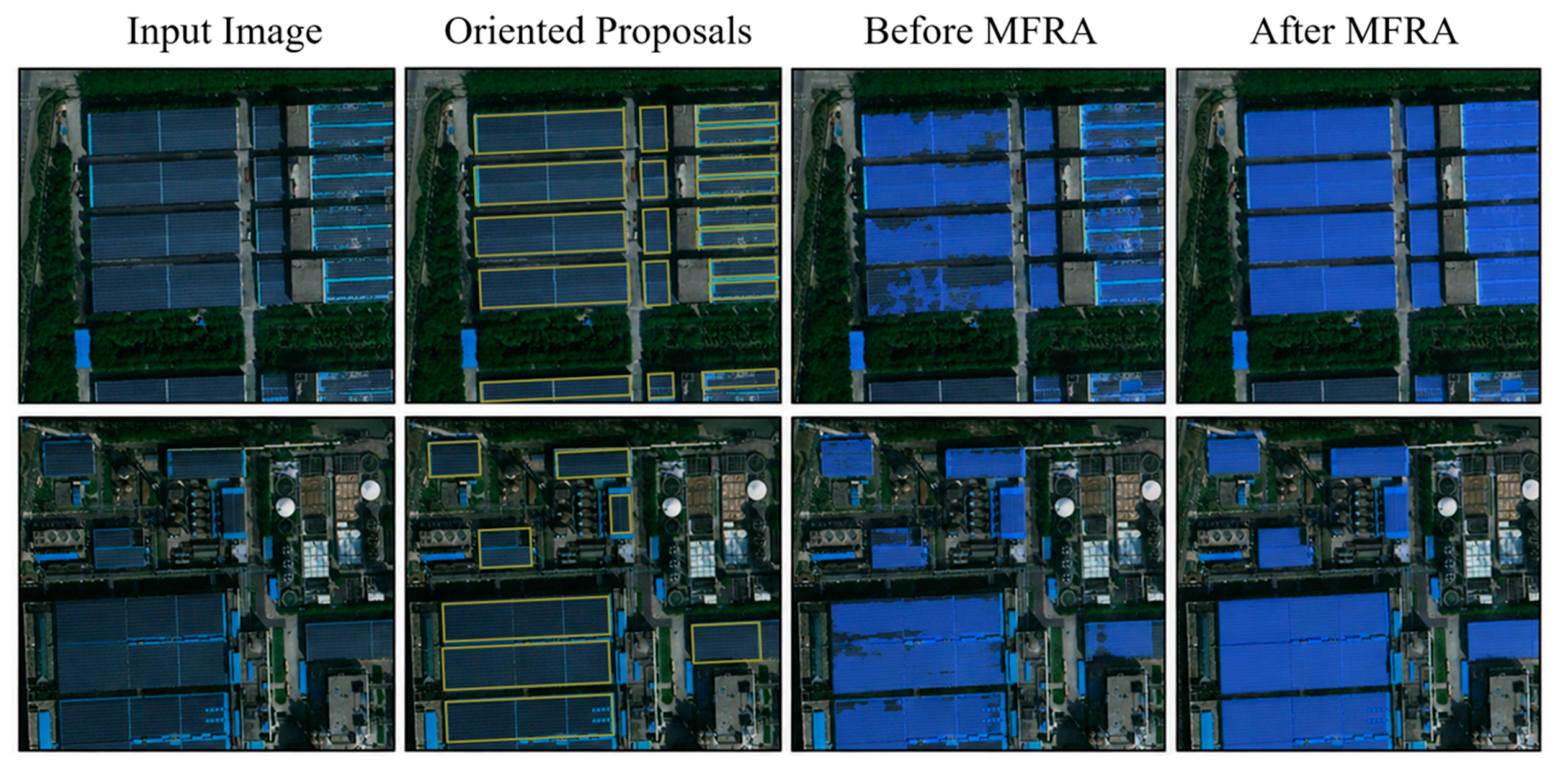
To illustrate local refinement, Figure 14 compares two PV scenes. MFRA produces more complete local masks and better preserves several fine boundaries within proposal-aligned RGB tiles. Each row shows the input image, oriented proposals, prediction before MFRA, and final refined prediction after MFRA.

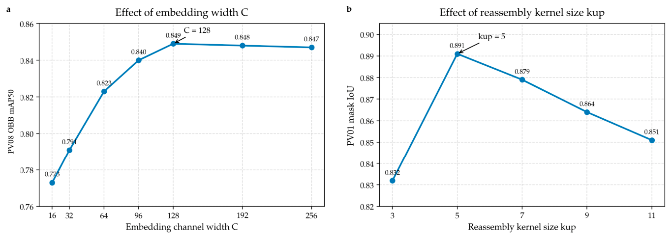
We further evaluated the sensitivity of embedding channel width C. As shown in Figure 15a, increasing C from 32 to 128 improves PV08 OBB mAP50 from 0.791 to 0.849. Increasing C to 256 yields no clear gain but increases parameter count and memory use. We therefore use C = 128.

We also examined the reassembly kernel size $k_{u\mathrm{p}}$. As shown in Figure 15b, $k_{u\mathrm{p}}$ = 3 provides insufficient local context and reduces PV01 mask IoU to 0.832. In contrast, $k_{u\mathrm{p}}$ = 7 introduces more background response and slightly weakens boundary precision. The final setting $k_{u\mathrm{p}}$ = 5 gives the best observed balance between local context and boundary preservation.

Physical GSD Embedding and GSD-conditioned spatial gating progressively improve representation quality on the PV08 tier. The proposal-guided local mask refinement pipeline primarily changes the inference path and reduces the cost of dense full-frame segmentation, while MFRA improves high-resolution mask refinement on PV01. The selected hyperparameters $C=128$ and $k_{\mathrm{u}\mathrm{p}}=5$ provide a practical balance between accuracy, computational cost, and boundary preservation.

A second ablation isolates GSD representation and injection position.

Table 5. Comparison of GSD-conditioning and fusion-stage reassembly alternatives.

Variant	GSD Cue	Conditioning/Reassembly	Macro OBB mAP50	Macro Mask IoU	Latency (ms)	FPS
A	None	Bilinear + Conv	0.861	0.779	32.9	30.4
B	None	Content-only CARAFE, $K\left(X\right)$	0.871	0.794	33.8	29.6
C	Normalized scalar	Pre-fusion concatenation	0.884	0.809	34.0	29.4
D	Tier one-hot	Tier conditioning	0.886	0.813	33.9	29.5
E	Continuous scalar	FiLM modulation	0.891	0.820	34.2	29.2
F	Sinusoidal	Post-reassembly spatial gate	0.896	0.827	34.7	28.8
G	Sinusoidal	Pre-kernel CRFA, $K(X,s_{\mathrm{e}\mathrm{f}\mathrm{f}})$.	0.902	0.833	35.2	28.4

reports macro performance over PV08, PV03, and PV01 together with measured PyTorch FP32 latency and throughput on the Jetson TX2.

Replacing bilinear fusion with content-only CARAFE increases macro OBB mAP50 from 0.861 to 0.871 and macro mask IoU from 0.779 to 0.794. Direct scalar concatenation, tier one-hot encoding, and continuous scalar FiLM further raise the two metrics to 0.884/0.809, 0.886/0.813, and 0.891/0.820 respectively. These results show that scale information is useful.

Conditioning before kernel prediction performs better than applying a GSD spatial gate after reassembly. With the same sinusoidal GSD encoding, macro OBB mAP50 rises from 0.896 to 0.902, and macro mask IoU rises from 0.827 to 0.833. These gains highlight the benefit of using GSD to guide local aggregation weights during kernel prediction. Compared with standard CARAFE, full CRFA improves the two metrics by 0.031 and 0.039, respectively, with an additional latency of 1.4 ms and a throughput of 28.4 FPS.

4.3. Controlled Validation and Statistical Robustness of GSD Conditioning

To validate the GSD-conditioned behavior and statistical robustness of CRFA-PVNet, this subsection combines controlled scale experiments with repeated-training analysis. The controlled evaluation includes same-scene resampling, GSD-input intervention, and testing at unseen intermediate GSDs. Statistical robustness is assessed through three independent training runs. A separate partition comparison evaluates the influence of random-patch splitting and the spatially disjoint protocol. Together, these analyses examine the response of CRFA-PVNet to sampling scale, GSD metadata, training stochasticity, and dataset partitioning.

The first experiment used held-out 0.1 m orthorectified scenes from the spatially disjoint test set. Each scene was resampled to 0.2, 0.3, 0.4, 0.6, and 0.8 m using anti-aliased area resampling. Models with and without CRFA were evaluated at all resolutions with their trained weights fixed. Following Section 3.3, $E_{CR}$ was calculated relative to the feature representation at 0.1 m for each model. 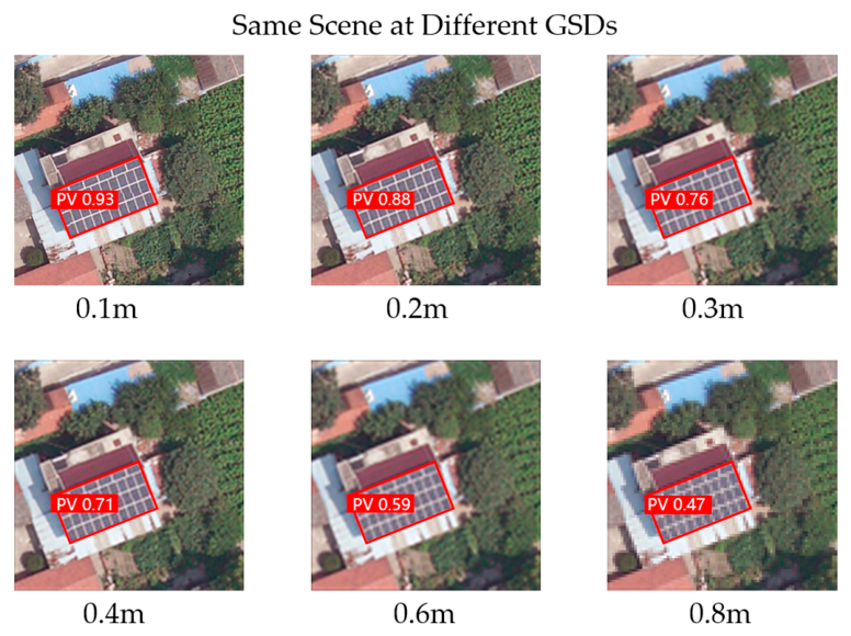Figure 16 illustrates how predictions change as the same scene is sampled at progressively coarser resolutions.

Table 6. Controlled same-scene evaluation across resampled GSD conditions.

GSD (m)	No CRFA OBB mAP50	CRFA OBB mAP50	No CRFA Mask IoU	CRFA Mask IoU	No CRFA E_CR	CRFA E_CR
0.1	0.938	0.945	0.887	0.892	0.000	0.000
0.2	0.923	0.934	0.866	0.879	0.058	0.043
0.3	0.901	0.919	0.838	0.856	0.095	0.068
0.4	0.876	0.902	0.801	0.828	0.132	0.093
0.6	0.829	0.865	0.741	0.782	0.205	0.142
0.8	0.774	0.824	0.667	0.724	0.278	0.187

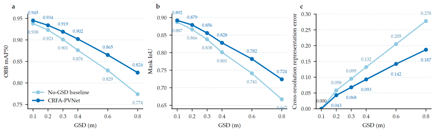
and Figure 17 show that detection and segmentation performance decline as resolution becomes coarser, while representation error increases. CRFA reduces $E_{CR}$ at every tested GSD above the 0.1 m reference. At 0.8 m, it lowers $E_{CR}$ from 0.278 to 0.187 and improves OBB mAP50 from 0.774 to 0.824. Mask IoU also increases from 0.667 to 0.724. With scene content and annotations held constant, these results show how CRFA improves feature alignment and prediction across sampling scales.

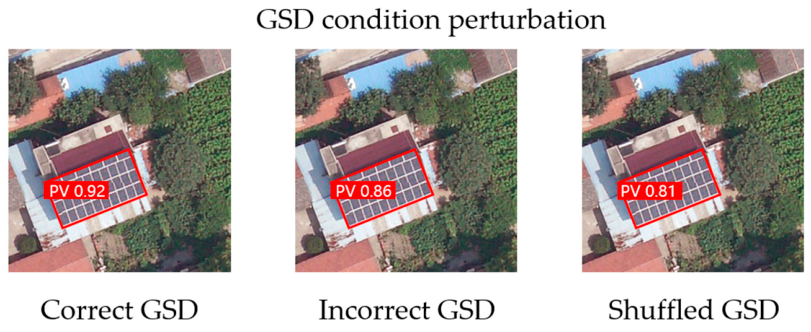
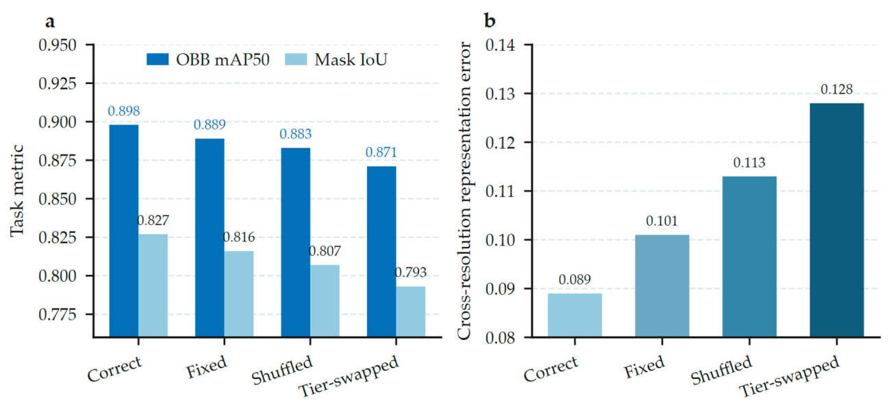
We next intervene on the GSD input while keeping images, labels, and trained weights fixed. Correct metadata is compared with a fixed 0.3 m value, five independently shuffled assignments, and an incorrect tier-swapped setting in which 0.1 and 0.8 m conditions are exchanged while 0.3 m is retained. Figure 18 shows a representative prediction under correct, incorrect, and shuffled GSD inputs.

Table 7. Intervention on the GSD conditioning input with images and weights fixed.

GSD Input	Macro OBB mAP50	Macro Mask IoU	Mean E_CR
Correct	0.898	0.827	0.089
Fixed at 0.3 m	0.889	0.816	0.101
Shuffled (five assignments)	0.883 ± 0.002	0.807 ± 0.002	0.113 ± 0.002
Incorrect tier-swapped	0.871	0.793	0.128

and Figure 19 show that predictions become less accurate as the GSD input departs from the correct values. Using a constant GSD of 0.3 m lowers macro OBB mAP50 and macro mask IoU by 0.009 and 0.011, respectively, and raises mean $E_{CR}$ by 0.012. Shuffling the GSD values causes larger accuracy losses of 0.015 and 0.020, with a 0.024 increase in mean $E_{CR}$. Swapping the tier values has the strongest effect: the two accuracy metrics fall by 0.027 and 0.034, while mean $E_{CR}$ increases by 0.039.

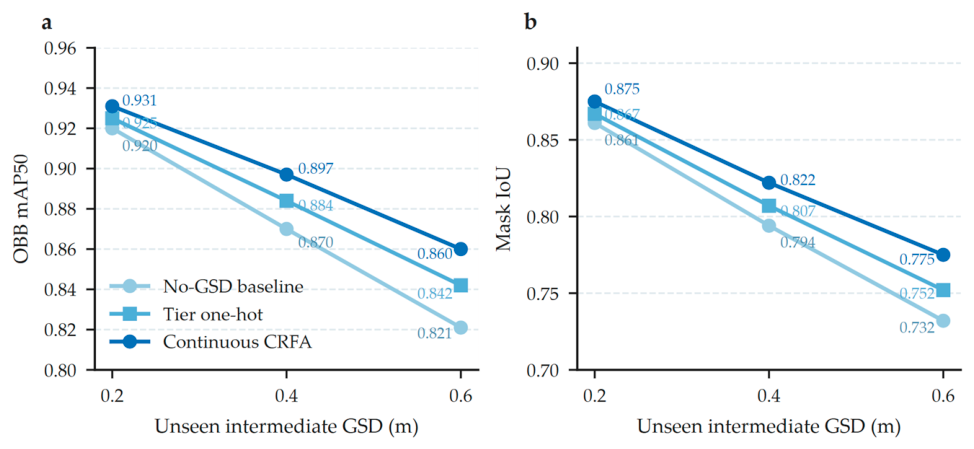
We then evaluated CRFA at unseen intermediate GSDs of 0.2, 0.4, and 0.6 m. Training used only the nominal 0.1, 0.3, and 0.8 m conditions, and the models were tested directly on the intermediate-resolution images without adaptation. This experiment compares continuous CRFA encoding with two alternatives: no GSD conditioning and discrete tier one-hot encoding.

Table 8. Strict evaluation at unseen intermediate GSDs.

Unseen GSD (m)	No GSD OBB mAP50	One-Hot OBB mAP50	CRFA OBB mAP50	No GSD Mask IoU	One-Hot Mask IoU	CRFA Mask IoU
0.2	0.920	0.925	0.931	0.861	0.867	0.875
0.4	0.870	0.884	0.897	0.794	0.807	0.822
0.6	0.821	0.842	0.860	0.732	0.752	0.775

and Figure 20 show that CRFA exceeds the no-GSD model by 0.011/0.014, 0.027/0.028, and 0.039/0.043 in OBB mAP50/mask IoU at 0.2, 0.4, and 0.6 m respectively. It also exceeds tier one-hot conditioning at all three unseen values, with the largest gains of 0.018 OBB mAP50 and 0.023 mask IoU at 0.6 m. The same-scene and metadata-intervention results demonstrate the value of matching the GSD input to the image sampling scale. The gains at unseen intermediate GSDs further show that CRFA extends cross-resolution prediction beyond the three nominal training tiers.

To evaluate sensitivity to training stochasticity, CRFA-PVNet and the strongest task-specific baselines were retrained with three random seeds under the same fixed spatially disjoint partition.

Table 9. Statistical robustness over three complete training runs.

Metric	Tier	Baseline Mean ± SD	CRFA-PVNet Mean ± SD	Paired Improvement [95% CI]
OBB mAP50	PV08	0.807 ± 0.002	0.849 ± 0.004	0.042 [0.027, 0.057]
OBB mAP50	PV03	0.889 ± 0.004	0.913 ± 0.001	0.024 [0.015, 0.033]
OBB mAP50	PV01	0.929 ± 0.003	0.944 ± 0.003	0.015 [0.013, 0.016]
OBB mAP50	Macro	0.875 ± 0.002	0.902 ± 0.002	0.027 [0.025, 0.029]
Mask IoU	PV08	0.610 ± 0.002	0.763 ± 0.005	0.153 [0.138, 0.168]
Mask IoU	PV03	0.736 ± 0.002	0.843 ± 0.003	0.107 [0.102, 0.113]
Mask IoU	PV01	0.821 ± 0.003	0.891 ± 0.002	0.070 [0.066, 0.073]
Mask IoU	Macro	0.722 ± 0.001	0.832 ± 0.003	0.110 [0.105, 0.115]

summarizes the resulting OBB mAP50 and mask IoU distributions.

Across the three runs, CRFA-PVNet retained higher OBB mAP50 and mask IoU than the strongest task-specific baseline at every GSD tier. The mean OBB mAP50 improvements were 0.042, 0.024, and 0.015 on PV08, PV03, and PV01 respectively, and the corresponding mask IoU improvements were 0.153, 0.107, and 0.070. All seed-matched 95% confidence intervals remained above zero under the fixed spatial partition, while the small between-run standard deviations indicate limited sensitivity to training stochasticity.

4.4. Quantitative Diagnostic of Spatial Information Leakage

We compared random-patch partitioning with the spatially disjoint buffer protocol to assess how data partitioning affects performance. Model architectures and training settings were kept identical across the two protocols. Predictions and annotations from PV08, PV03, and PV01 were pooled to calculate OBB mAP50.

Table 10. Descriptive validation-test performance gaps under random and spatially disjoint partitioning.

Model	Partition Protocol	Pooled Validation OBB mAP50	Pooled Cross-Regional Test OBB mAP50	Validation-Test Performance Gap
YOLOv10-B	Random-patch partitioning	0.862	0.712	+0.150
YOLOv10-B	Spatially disjoint buffer	0.754	0.748	+0.006
RT-DETR-L	Random-patch partitioning	0.881	0.743	+0.138
RT-DETR-L	Spatially disjoint buffer	0.771	0.765	+0.006
Oriented R-CNN	Random-patch partitioning	0.894	0.781	+0.113
Oriented R-CNN	Spatially disjoint buffer	0.812	0.805	+0.007
Ours	Random-patch partitioning	0.935	0.872	+0.063
Ours	Spatially disjoint buffer	0.884	0.879	+0.005

presents the validation and cross-regional test results, along with the differences between them.

Random partitioning produces larger validation-test gaps for all baselines. YOLOv10-B obtains 0.862 validation OBB mAP50 and 0.712 cross-regional test OBB mAP50, a gap of +0.150. RT-DETR-L and Oriented R-CNN show the same general pattern. These results are consistent with spatial dependence among neighboring patches, although regional differences in scene composition and image acquisition may also contribute.

The spatially disjoint protocol gives lower validation scores, but validation and cross-regional test scores are closer. The gap falls from +0.150 to +0.006 for YOLOv10-B, from +0.138 to +0.006 for RT-DETR-L, and from +0.113 to +0.007 for Oriented R-CNN. These descriptive changes indicate reduced partition sensitivity, not a causal estimate of spatial leakage alone.

CRFA-PVNet has a random-partition gap of +0.063 and a spatially disjoint gap of +0.005. The smaller descriptive gap indicates closer validation and cross-regional test performance under geographic separation. It does not show that model design alone removes spatial dependence.

The analysis shows that random-split accuracy can be optimistic in PV remote sensing because adjacent patches share environmental context. It also supports geographically separated validation when cross-regional performance is the target. All results in Table 3 use the spatially disjoint protocol, which limits direct neighborhood reuse between subsets.

4.5. Edge Deployment Performance, Proposal-Budget Sensitivity, and Runtime Analysis

The complete CRFA-PVNet was profiled on an NVIDIA Jetson TX2 after warm-up under the same standardized single-frame inference setting used for Table 4. The final model contains 24.5 million parameters and requires 38.2 GFLOPs. Because the local mask branch is activated only for selected proposals, the per-frame workload varies with the number of valid proposals. The memory-aware top-N selection and fixed-size local batching described in Section 3.5 keep tensor dimensions and peak memory within a controlled range. To separate runtime-level acceleration from the architectural efficiency analyzed in Table 4, the same trained CRFA-PVNet weights were evaluated using PyTorch FP32, TensorRT FP32, and TensorRT FP16 [51]. All variants used identical input data, proposal thresholds, Nmax, and post-processing settings.

Under the native PyTorch FP32 implementation, the measured end-to-end latency was 35.2 ms per frame. Full-frame oriented proposal generation required 11.4 ms, RoI affine transformation and bilinear sampling required 3.4 ms, and local segmentation with MFRA required 20.4 ms. The resulting throughput was 28.4 FPS, with a measured average power draw of 14.2 W and a peak device memory of 4.21 GB.

The architectural ablation in Table 4 shows that proposal-guided local refinement reduces the cost of full-frame segmentation; the following comparison evaluates the additional gains from inference-runtime optimization.

Table 11. Cross-runtime deployment performance of CRFA-PVNet on the NVIDIA Jetson TX2.

Inference Backend	Precision	Macro OBB mAP50	Macro Mask IoU	Latency (ms)	FPS	Peak Memory (GB)	Power (W)
PyTorch	FP32	0.902	0.833	35.2	28.4	4.21	14.2
TensorRT	FP32	0.902	0.833	28.7	34.8	4.08	14.3
TensorRT	FP16	0.900	0.831	24.2	41.3	3.74	14.4

compares the same Seed 2 CRFA-PVNet model across inference backends and numerical precisions. TensorRT FP32 reduces end-to-end latency from 35.2 to 28.7 ms and increases throughput from 28.4 to 34.8 FPS, corresponding to a 1.23× speedup over PyTorch FP32.

Enabling TensorRT FP16 further reduced latency to 24.2 ms and increased throughput to 41.3 FPS, yielding an overall speedup of 1.45×. Peak device memory decreased from 4.21 GB to 3.74 GB. The macro OBB mAP50 and macro mask IoU decreased by 0.002, indicating a limited numerical-precision effect across the three GSD tiers.

Average board power remained similar across the three deployment settings, increasing slightly from 14.2 W to 14.4 W under TensorRT FP16. Because throughput increased, the energy per processed frame decreased from 0.500 J to 0.349 J, corresponding to a 30.2% reduction. The PyTorch FP32-to-TensorRT FP16 comparison changes both the inference backend and numerical precision; therefore, the overall improvement reflects their combined effects, whereas TensorRT FP32 separately indicates the runtime-level contribution.

To quantify how the proposal budget affects segmentation completeness and edge resource use, $N_{max}$ was varied among 4, 8, 16, 24, and 32. All accuracy measurements used TensorRT FP16. A separate fixed-shape engine was constructed for each proposal capacity, and unused local-mask slots were zero-padded. Proposal recall was measured at a rotated-IoU threshold of 0.5. End-to-end mask IoU was calculated after projecting the local predictions back to the original image; ground-truth instances missed by the proposal branch remained in the reference mask and therefore contributed false-negative regions. Mean active proposals denotes the average number of valid regions processed per image. Runtime measurements followed the standardized single-frame Jetson TX2 protocol used for Table 11.

Table 12. Effect of the active-proposal limit on proposal recall and end-to-end mask segmentation across the three GSD tiers.

${\mathit{N}}_{\mathit{m}\mathit{a}\mathit{x}}$	Mean Active Proposals/Image	Proposal Recall@0.5				End-to-End Mask IoU
		PV08	PV03	PV01	Macro	PV08	PV03	PV01	Macro
4	2.82	0.678	0.760	0.840	0.759	0.690	0.776	0.850	0.772
8	3.17	0.796	0.873	0.923	0.864	0.748	0.830	0.882	0.820
16	3.20	0.809	0.885	0.931	0.875	0.759	0.839	0.888	0.829
24	3.20	0.810	0.887	0.932	0.876	0.761	0.841	0.889	0.830
32	3.20	0.811	0.887	0.932	0.877	0.762	0.841	0.889	0.831

shows that increasing the proposal budget improves instance coverage and end-to-end segmentation quality, with diminishing gains at higher capacities. Increasing $N_{\mathrm{m}\mathrm{a}\mathrm{x}}$ from 4 to 8 raises macro proposal recall from 0.759 to 0.864 and macro mask IoU from 0.772 to 0.820. Both metrics approach a plateau at $N_{\mathrm{m}\mathrm{a}\mathrm{x}}=16$, reaching 0.875 and 0.829, respectively. The larger improvements on PV08 and PV03 indicate that retaining additional candidates is particularly beneficial for the coarser imagery.

Table 13. Effect of the configured local proposal capacity on TensorRT FP16 deployment performance on the NVIDIA Jetson TX2.

${\mathit{N}}_{\mathit{m}\mathit{a}\mathit{x}}$	Latency (ms)	FPS	Peak Memory (GB)
4	19.8	50.5	3.18
8	20.5	48.8	3.27
16	21.7	46.1	3.43
24	23.0	43.5	3.59
32	24.2	41.3	3.74

shows that increasing $N_{\mathrm{m}\mathrm{a}\mathrm{x}}$ from 4 to 32 raises latency from 19.8 to 24.2 ms and peak memory from 3.18 to 3.74 GB. Among the evaluated settings, $N_{\mathrm{m}\mathrm{a}\mathrm{x}}=16$ offers an efficient balance between segmentation quality and resource use. Compared with $N_{\mathrm{m}\mathrm{a}\mathrm{x}}=32$, it reduces latency by 2.5 ms and peak memory by 0.31 GB, while macro proposal recall and macro mask IoU each decrease by only 0.002.

Together, these results show that runtime optimization and proposal-guided refinement provide complementary improvements in deployment efficiency. TensorRT FP16 accelerates inference, while the proposal budget provides an explicit means of balancing instance coverage, segmentation quality, latency, and memory use.

4.6. Cross-Dataset Evaluation on Independent Aerial Orthophotos

We selected 50 complete aerial orthophotos at 0.3 m GSD from the Duke Solar Array Dataset [4] to evaluate cross-dataset transfer. These images formed an external test set independent of PV01, PV03, and PV08. They were used exclusively for testing and played no role in training, validation, fine-tuning, or the selection of thresholds and hyperparameters.

Each complete orthophoto was partitioned offline into 25 non-overlapping tiles to match the network’s fixed input size. This produced 1250 external test tiles. The official PV polygons were converted into instance masks for each tile, with minimum-area rotated rectangles serving as the corresponding OBB annotations. CRFA-PVNet was then evaluated on all external tiles with its trained weights frozen and the effective GSD set to 0.3 m. Inference and post-processing followed the same protocol as the main evaluation.

As shown in

Table 14. Frozen-model cross-dataset evaluation on 50 independent 0.3 m Duke aerial orthophotos.

Dataset	GSD	Precision	Recall	F1-Score	OBB mAP50	Mask IoU
Duke Solar Array	0.3 m	0.881	0.823	0.851	0.861	0.780

, the frozen CRFA-PVNet achieved a precision of 0.881, a recall of 0.823, an F1-score of 0.851, an OBB mAP50 of 0.861, and a mask IoU of 0.780 on the 1250 external test tiles. The model maintained effective detection and segmentation performance on independently sourced aerial imagery containing previously unseen roof structures and PV layouts. This frozen-model evaluation demonstrates the cross-dataset transfer capability of CRFA-PVNet without target-domain adaptation.

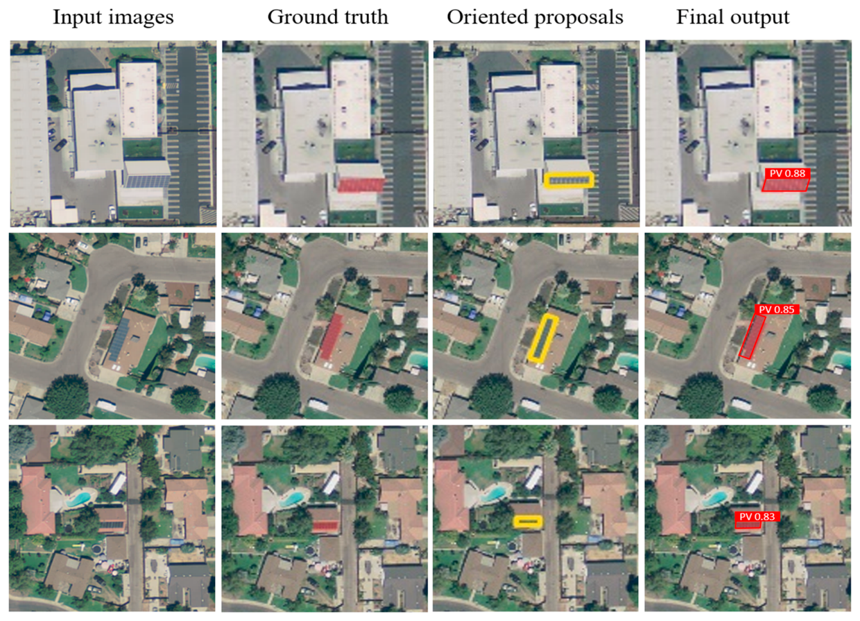
Figure 21 compares representative predictions on the external dataset with the official Duke annotations. The oriented boxes capture the shape and orientation of PV arrays. The proposal-guided mask branch delineates the panel regions despite the unfamiliar backgrounds and roof layouts.

The three examples contain PV arrays with different sizes, aspect ratios, and surrounding roof structures. CRFA-PVNet detects all three instances with confidence scores ranging from 0.83 to 0.88. The predicted orientations follow the principal axes of the annotated arrays, including the elongated installation in the second example. These qualitative results complement Table 14 by showing that the frozen model preserves PV geometry across independently sourced aerial scenes.

5. Conclusions

This paper proposes CRFA-PVNet for PV detection and segmentation across satellite, aerial, and UAV images. The physical receptive-field formulation relates pixel-level sampling to ground span and guides the introduction of effective GSD into feature reassembly at the multi-scale fusion stage. By conditioning spatial features before local-kernel prediction, CRFA makes the aggregation weights responsive to both image content and physical sampling scale. This design enables a single jointly trained model to process imagery at different resolutions, while proposal-guided local mask refinement concentrates boundary prediction on selected PV regions.

Experiments under the spatially disjoint protocol demonstrate improvements in both oriented detection and mask segmentation across the three GSD tiers, with the largest gains on the coarse PV08 imagery, where OBB mAP50 and mask IoU reach 0.849 and 0.764, respectively. Controlled resampling and GSD-input interventions show that matching physical-scale information to the image improves feature alignment and prediction, while tests at unseen intermediate GSDs demonstrate the effectiveness of conditioning beyond the nominal training resolutions. The frozen model also achieves 0.861 OBB mAP50 and 0.780 mask IoU on independent Duke aerial imagery, demonstrating cross-dataset transfer without target-domain adaptation. On an NVIDIA Jetson TX2, TensorRT FP16 deployment reaches 41.3 FPS with 3.74 GB peak memory, with macro OBB mAP50 and macro mask IoU each only 0.002 below their TensorRT FP32 values.

CRFA-PVNet is designed for orthorectified imagery with locally stable ground resolution. Severe blur and very small PV installations can weaken proposal generation by suppressing the fine spatial evidence needed for reliable localization. Low panel-to-background contrast and partial occlusion may reduce proposal confidence and lead to incomplete or fragmented masks. Regular roof textures and reflective surfaces can produce PV-like responses and false detections. Research will also extend to effective GSD estimation from incomplete metadata and evaluation across additional regions, sensors, acquisition conditions, and edge platforms. Integrating automated orthophoto tiling and cross-tile result consolidation will support more convenient application of the framework to large-area PV mapping.