Downscaling of SMAP Soil Moisture Based on the Transformer Algorithm in Anhui Province

Highlights

A Transformer-based framework was built for soil moisture (SM) downscaling. Transformer and its variants (PatchTST and iTransformer) outperformed RF, LSTM, and CNN-LSTM in SM downscaling tasks. Validated against in situ SM, Transformer-downscaled SM outperformed 9 km SMAP and SMCI1.0. Land surface temperature difference and groundwater level greatly impact SM.

What are the main findings?

• Transformer and its variants (PatchTST and iTransformer) demonstrated superior downscaling performance compared with RF, LSTM, and CNN-LSTM.
• Land surface temperature difference and groundwater level greatly impact SM.

What are the implications of the main findings?

• The Transformer-based downscaling framework provides an effective approach for generating high-resolution SM data from coarse-resolution satellite products.
• The generated high-accuracy daily 1 km SM dataset can support regional hydrological monitoring, agricultural drought assessment, and related environmental studies.

Abstract

Soil moisture (SM) is critical for climate, water, and agriculture, but Soil Moisture Active Passive (SMAP) passive microwave products have coarse resolution, limiting regional applications. This study develops an SM downscaling framework based on Transformer and its variants (PatchTST and iTransformer), integrating multi-source satellite and groundwater data to generate 1 km daily SM products (2015–2022). Compared with Random Forest (RF), Long Short-Term Memory (LSTM), and Convolutional Neural Network–LSTM (CNN-LSTM), Transformer and its variants achieve superior accuracy and generalization. Validated against in situ measurements and SMCI1.0, the Transformer-downscaled SM product achieved the best accuracy with ubRMSE = 0.0372 m³/m³ and RMSE = 0.0591 m³/m³. The downscaled SM dataset not only captured finer spatial details but also preserved the spatial patterns and seasonal dynamics of the original SMAP product and showed good responsiveness to precipitation events. Feature importance analysis revealed that, aside from precipitation, the diurnal land surface temperature difference had a greater impact on SM than individual daytime or nighttime land surface temperature, ranking just below vegetation indices and soil texture factors, while groundwater level showed higher importance than elevation and surface temperature. This study confirms the effectiveness of Transformer-based models for SM spatial downscaling, providing a novel framework integrating remote sensing and deep hydrological information to generate accurate 1 km SM products.

1. Introduction

Soil moisture (SM) is a key variable linking energy and water exchange among the atmosphere, vegetation, and soil. It plays an essential role in hydrological process simulation, climate change research, water resource management, and agricultural activities [1,2,3,4]. Accurate SM monitoring is critical for improving the prediction and response efficiency of extreme natural disasters such as droughts, floods, and heatwaves [5,6,7,8].

Early SM data were obtained through traditional in situ measurement methods, including the oven-drying method and tensiometry [3,5]. Although such data feature high accuracy, their spatial representativeness and temporal continuity are severely limited [9,10,11]. Driven by the urgent demand for large-scale SM monitoring and advances in remote sensing technology [12,13,14,15], optical and microwave remote sensing have been gradually applied to SM monitoring [16,17]. Optical remote sensing indirectly retrieves SM by measuring surface reflectance in solar reflective bands (visible, near-infrared, and shortwave infrared) [18] and thermal radiation in the thermal infrared band [9,19,20]. However, optical remote sensing is easily disturbed by cloud cover, atmospheric conditions, and vegetation canopy, which greatly restricts its application in SM retrieval. To better monitor SM variations, microwave remote sensing compensates for the shortcomings of optical remote sensing owing to its unique advantages, such as low atmospheric interference and strong penetration capability [5,16,17]. Active microwave remote sensing mainly relies on synthetic aperture radar (SAR) to obtain surface backscattering coefficients and retrieves SM using its relationship with soil dielectric permittivity and water content. Passive microwave remote sensing measures the naturally emitted brightness temperature of soil via microwave radiometers and performs retrieval based on its correlation with SM [17,21]. Among these techniques, L-band passive microwave remote sensing exhibits higher sensitivity to SM dynamics and better signal-to-noise ratio than radar and optical remote sensing [9,22], making it a research hotspot in SM monitoring. The Soil Moisture Active Passive (SMAP) mission, a typical representative of L-band passive remote sensing satellites, has been successfully used for global SM monitoring.

However, microwave remote sensing SM products suffer from limited spatial resolution, which makes it difficult to meet the high-precision application requirements of small-scale regions. In recent years, numerous studies have explored SM downscaling methods, which effectively improve the spatial resolution of SM products by fusing multi-source high-resolution data [1,23,24,25]. According to the different spatial downscaling models adopted in the downscaling framework, existing SM downscaling methods can be generally classified into three categories: empirical, semi-empirical, and physically based methods [26]. Among them, machine learning algorithms, as commonly used empirical downscaling approaches, show strong advantages in processing massive data and constructing reasonable downscaling models [5,27,28], and their effectiveness in downscaling has been widely validated. Early studies commonly used traditional machine learning methods such as Random Forest (RF), Support Vector Machine (SVM), and Gradient Boosting Decision Tree (GBDT) to implement SM downscaling for various study areas and original SM products, achieving satisfactory performance [23,29]. With the development of artificial neural networks, Convolutional Neural Networks (CNNs) [30], Long Short-Term Memory (LSTM) [31], and improved models integrating the two have been widely applied to SM prediction and downscaling [32,33,34,35]. Although these models perform well in spatial and temporal feature extraction, they still have certain limitations in capturing long-range dependencies and multivariate interactions [32,36]. The recently emerged Transformer model exhibits powerful long-range dependency modeling capability in multivariate time series analysis [37,38]. It supports parallel computation and offers distinct advantages in modeling complex variable interactions [39,40]. However, most current studies applying the Transformer model and its variants to SM-related research focus on root-zone or surface SM prediction, while applications to SM downscaling remain scarce. This gap highlights the need to further explore the potential of Transformer-based models in SM spatial downscaling.

In this study, by integrating multi-source remote sensing data and introducing diurnal land surface temperature difference and groundwater level, the applicability of the Transformer and its variants for SM downscaling was systematically evaluated, and an effective Transformer-based SM downscaling framework was constructed. Anhui Province, characterized by diverse landform features, was selected as the study area. Using data from 2015 to 2022, the 9 km resolution SMAP SM product was downscaled to 1 km resolution, yielding a higher-accuracy 1 km daily SM product that provides reliable data support for regional drought monitoring. The structure of the rest of this paper is as follows: Section 2 describes the study area and datasets; Section 3 introduces the data preprocessing procedure and the models used; Section 4 presents a comparative analysis of the accuracy of different downscaled SM products and validates their response to precipitation events; Section 5 explores the effects of various downscaling factors on SM and discusses the uncertainties in this study; Section 6 summarizes the main findings.

2. Study Area and Data

2.1. Study Area

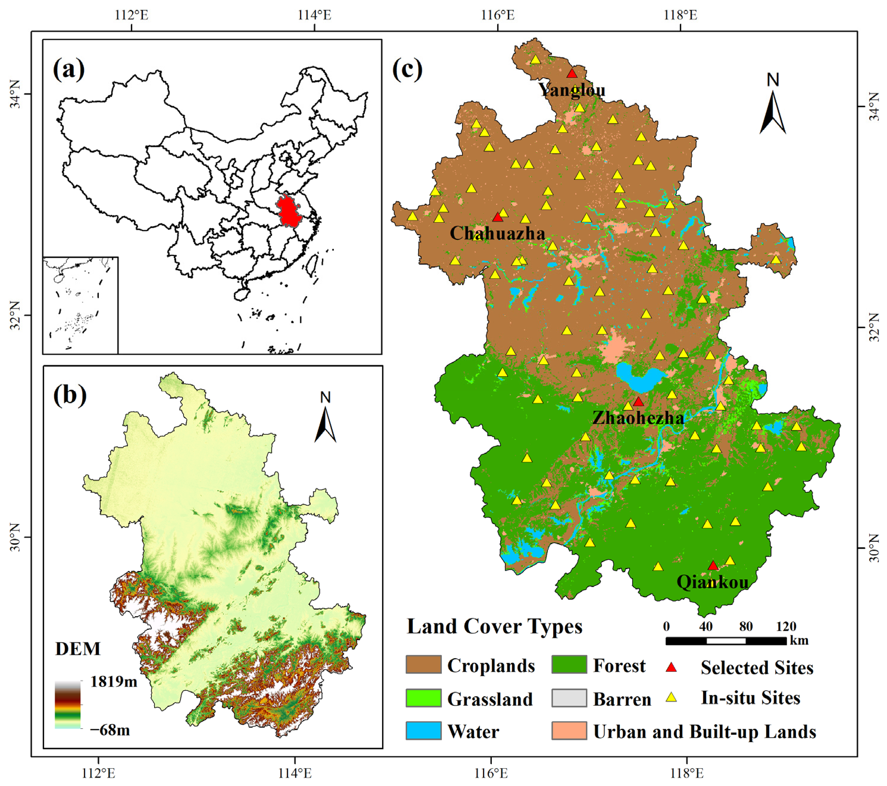
The study area is Anhui Province (114°54′–119°37′E, 29°41′–34°38′N), located in eastern China between the Yangtze River and Huaihe River. It serves as a transportation hub connecting east, west, south, and north China. Its location, elevation, and land cover types are shown in Figure 1. The total area of the province is approximately 140,100 km², with diverse geomorphic features characterized by mountainous south, hilly central, and plain north. The southern part is dominated by the Wannan Mountains with large topographic fluctuations; the central part consists of the Jianghuai Hills; and the northern part is dominated by the Huaibei Plain with relatively flat terrain. Anhui Province has a subtropical humid monsoon climate with distinct four seasons. Precipitation is concentrated in summer, with an average annual precipitation of about 800–1600 mm [41,42], showing significant spatial climatic differences. The study area is characterized by complex landforms and remarkable variations in hydro-meteorological conditions.

2.2. Data

In this study, various variables covering the study area were collected, including: daytime and nighttime land surface temperature (LST-Day, LST-Night), normalized difference vegetation index (NDVI), enhanced vegetation index (EVI), leaf area index (LAI), land cover (LC), DEM, soil texture (Sand, Silt, Clay), precipitation, and SMAP SM data. In addition, groundwater level (GW) and land surface temperature difference (LST-Diff) were introduced and collected. In situ-measured SM data for validating the accuracy of downscaled SM products and the soil moisture over China based on the In situ Data, Version 1.0 (SMCI1.0) SM product for accuracy comparison were also compiled. Detailed information on the data products corresponding to each variable is listed in

Table 1. Overview of data products and basic information used in this study.

Data Products	Temporal Resolution	Spatial Resolution	Related Variables	Time Range
MOD13Q1	16 days	250 m	NDVI	2000–present
			EVI
MOD15A2H	8 days	500 m	LAI	2000–present
MCD12Q1	Yearly	500 m	LC	2001–present
TRIMS LST	Daily	1 km	LST-Day	2000–2024
			LST-Night
			LST-Diff
CHIRPS 2.0	Daily	0.05°	Prep	1981–present
GWs_cn_1km	Monthly	1 km	GW	2005–2022
SMAP L4-SM	3 h	9 km	SM	2015–present
SMCI1.0 SM	Daily	1 km	SM	2000–2022
In situ SM	1st, 10th, 21st each month	Point-based observations	SM	2019
ASTER GDEM V3	-	30 m	DEM	-
China Soil Texture Dataset	-	1 km	Sand	-
			Silt
			Clay

Note: The “Related Variables” column shows the abbreviations of each variable; their full names have been introduced in Section 2.2.

.

Notably, the in situ SM observation data obtained for Anhui Province are only available for 2019. Therefore, the analysis of model downscaling results and validation against in situ data in this paper were conducted based on the reference year 2019. After determining the optimal downscaling model, the maximum overlapping time period was selected according to the temporal coverage of each input variable data product to construct a long-time-series downscaling dataset. The SMAP SM data have been available since April 2015, while the GW data were updated to 2022. Meanwhile, other auxiliary variables (e.g., LST-related variables, vegetation indices, DEM, precipitation) were fully covered during this period. Accordingly, this study finally obtained a high-precision, daily downscaled SM dataset with a spatial resolution of 1 km covering April 2015 to December 2022.

2.2.1. SMAP Level-4 SM Product

The SMAP Level-4 SM product (SMAP L4-SM) integrates L-band brightness temperature observations from the SMAP satellite with NASA’s Catchment land surface model through data assimilation, providing global surface (0–5 cm) and root-zone (=11,000 cm) SM data at a spatial resolution of 9 km and a temporal resolution of 3 h. Previous studies have confirmed its accuracy and reliability [43,44]. In this study, surface SMAP L4-SM data were obtained from the National Snow and Ice Data Center (NSIDC, https://nsidc.org/data/smap (accessed on 10 December 2025)).

2.2.2. MODIS

The Moderate Resolution Imaging Spectroradiometer (MODIS) features 36 spectral bands and offers products with spatial resolutions of 250 m, 500 m, and 1 km. It is one of the commonly used optical remote sensing datasets in SM spatial downscaling studies [17,45]. The relevant MODIS products considered in this study are listed in Table 1. Specifically, the MOD13Q1 product provides NDVI and EVI data at 250 m spatial resolution every 16 days; the MOD15A2H product offers LAI data at 500 m spatial resolution every 8 days; and the MCD12Q1 product supplies land cover (LC) data at 500 m spatial resolution. In this study, LC was not used as a model input variable but was utilized to characterize surface heterogeneity and provide background information for interpreting spatial variations in SM. All these data are publicly available from the Level-1 and Atmosphere Archive and Distribution System (LAADS, https://ladsweb.modaps.eosdis.nasa.gov/).

2.2.3. TRIMS LST

The land surface temperature (LST) data used in this study are from the Thermal and Reanalysis Integrating Moderate-resolution Spatial-Seamless LST (TRIMS LST) product. This dataset is generated by fusing Terra/Aqua MODIS LST products with Global Land Data Assimilation System (GLDAS) reanalysis data, featuring a spatial resolution of 1 km and four daily observations, covering mainland China and surrounding areas [46]. The LST-related variables involved in this study include LST-Day, LST-Night, and LST-Diff. The TRIMS LST product is publicly available from the National Tibetan Plateau Data Center (https://data.tpdc.ac.cn/).

2.2.4. Groundwater Level

This study incorporates the GW data product “GWs_cn_1km” released by the National Tibetan Plateau Data Center. This dataset provides monthly GW information for China at a 1 km spatial resolution, covering the period from 2005 to 2022 [47]. The data were obtained and included as one of the influencing factors in the SM spatial downscaling modeling to investigate the impact of groundwater dynamics on surface SM distribution.

2.2.5. Precipitation

This study uses the Climate Hazards Group InfraRed Precipitation with Station data (CHIRPS) version 2.0, which was originally developed to support the United States Agency for International Development (USAID) Famine Early Warning System Network (FEWS NET), and has since been widely applied in climate, drought, and hydrometeorological research [48]. In this study, the data were obtained via Google Earth Engine (GEE, https://developers.google.cn/earth-engine (accessed on 15 December 2025)) with a spatial resolution of 0.05° and a temporal resolution of 1 day.

2.2.6. Topography and Soil Texture

To characterize the topographic features of the study area, we incorporated DEM data from the Advanced Spaceborne Thermal Emission and Reflection Radiometer Global Digital Elevation Model Version 3 (ASTER GDEM V3) product, which has a spatial resolution of 30 m and is characterized by high accuracy and broad spatial coverage. The soil texture data were generated based on the 1:1,000,000 soil map of China and 8595 soil profile records from the Second National Soil Survey, and were obtained from the Global Resource Data Cloud Platform (http://www.gis5g.com), with a spatial resolution of 1 km.

2.2.7. In Situ Observation Data and SMCI1.0 SM

To evaluate the accuracy of the downscaled SM products, this study used two types of reference data: in situ SM observations from ground monitoring stations and an independent 1 km resolution SM product, SMCI1.0 SM.

The in situ data were obtained from the Anhui Provincial Hydrology Bureau, including SM measurements from 87 observation stations during the period from April to August 2019. Observations were recorded at 8:00 a.m. on the 1st, 10th, and 21st of each month, and SM was measured using the gravimetric method at three standard depth layers: 10 cm, 20 cm, and 40 cm. Considering the relatively close soil layer depth of the in situ measurements to the SMAP L4-SM product and following previous validation practices, the 10 cm measurements were selected for accuracy validation in this study. SMCI1.0 is a 1 km daily SM product independently developed in China, constructed based on data from 1648 ground stations and multiple auxiliary variables [49]. It serves as an important reference for evaluating the performance of the downscaled SM products at the regional scale. This dataset is publicly available from the National Tibetan Plateau Data Center (https://data.tpdc.ac.cn/).

3. Methods

3.1. SM Spatial Downscaling Framework

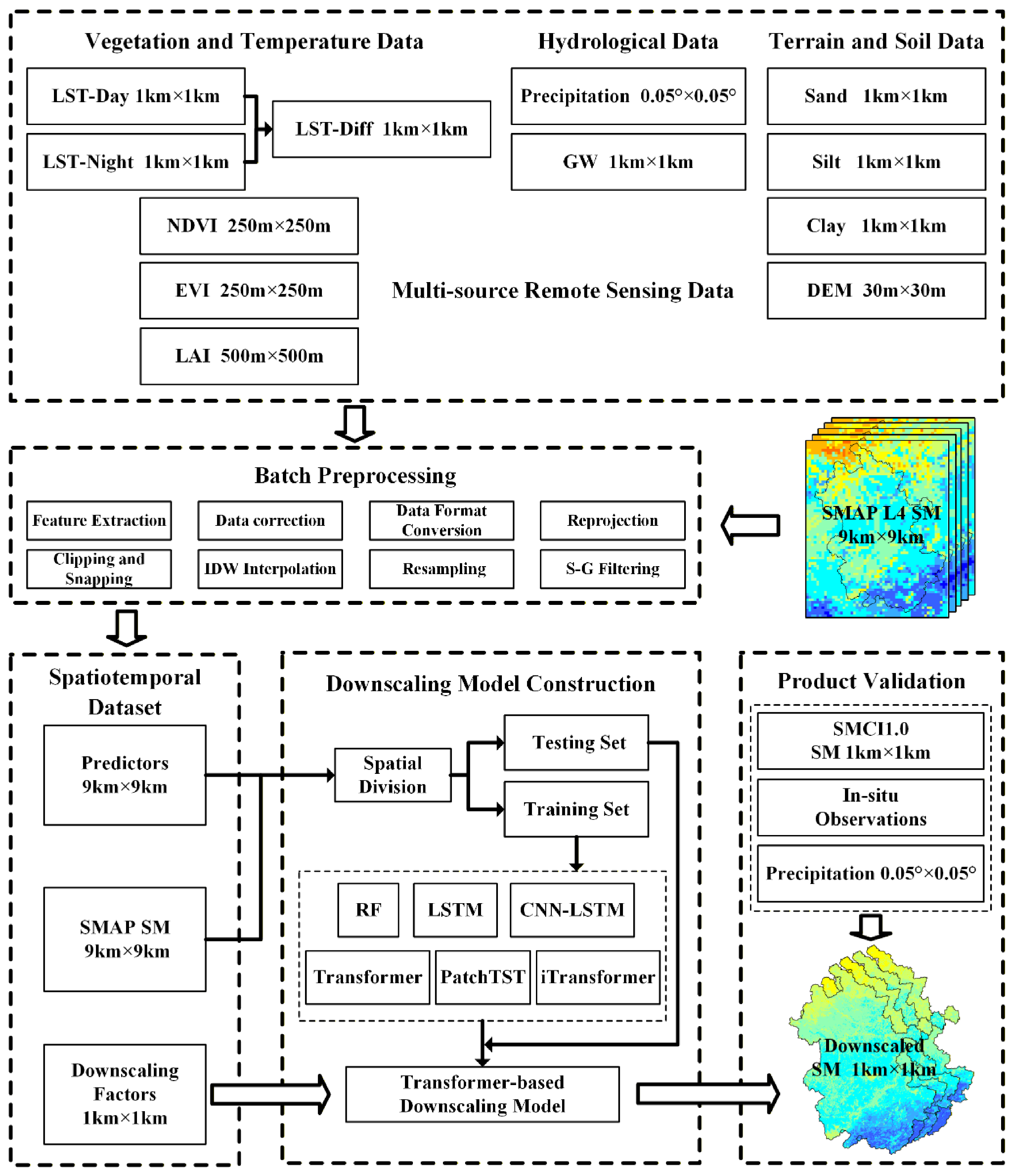
SM downscaling studies are often based on the assumption that spatial scale does not affect the mapping relationship between SM and auxiliary variables [1,50]. The SM downscaling framework of this study is shown in Figure 2, which mainly includes four parts: data acquisition, data preprocessing, downscaling model training, and accuracy evaluation of downscaled SM products. In the data preprocessing stage, to address inconsistencies in the temporal resolution of different auxiliary variables, Savitzky–Golay (S-G) filtering (window length = 15, fourth-order polynomial) and linear temporal interpolation were applied to NDVI, EVI, LAI, and GW time series to reduce noise and harmonize their temporal resolutions, generating continuous daily auxiliary variables for model input. For model training and testing, the study area was divided into 68 spatial blocks of 50 km × 50 km, with 54 blocks used for training and 14 blocks used for testing. In the model training stage, the coarse-resolution SM product was used as supervision, and Transformer-based deep learning methods were adopted to model multi-source time-series variables, with comparative analysis conducted against RF, LSTM, and CNN-LSTM models. Finally, through validation against in situ observation data and the SMCI1.0 SM product, the accuracy of the Transformer-based downscaled SM product was evaluated to demonstrate the effectiveness and applicability of the Transformer downscaling model.

3.2. Transformer and Its Variants

3.2.1. Transformer Model

The Transformer model was first proposed by Vaswani, Shazeer, Parmar, Uszkoreit, Jones, Gomez, Kaiser, and Polosukhin [38] and has attracted widespread attention due to its outstanding performance in the field of natural language processing (NLP). With the continuous advancement of research, Transformer models have gradually been extended to time series forecasting tasks [40,51], demonstrating excellent predictive performance and strong generalization capability in modeling temporal dependencies and multivariate interactions. In SM downscaling studies, the inputs usually consist of multi-source heterogeneous temporal variables, which exhibit significant temporal correlations and inter-variable coupling characteristics. Therefore, the introduction of Transformer models into SM downscaling is theoretically well suited for this task.

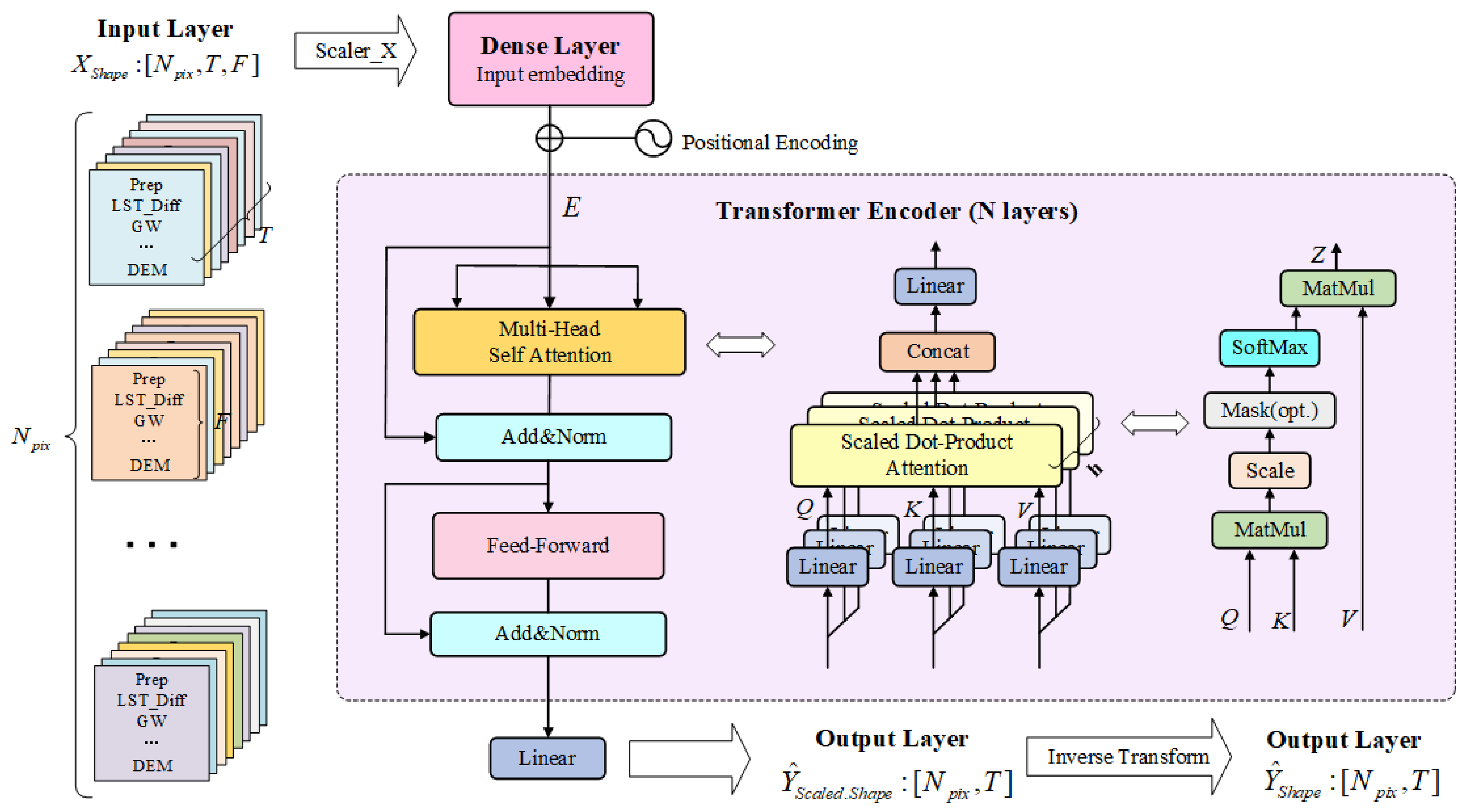
This study employed a Transformer model based on the Encoder architecture, and the overall structure of the model is shown in Figure 3. During the training process of the SM downscaling model, the input data were organized as a three-dimensional tensor: $X\in R^{N_{pix}\times T\times F}$, where $N_{pix}$ denotes the number of pixels in Anhui Province, $T$ represents the number of time steps, and $F$ indicates the number of SM influencing factors, totaling 12 variables. The input data were processed through modules including positional encoding (PE), Multi-Head Self-Attention, and a feed-forward network to generate the predicted SM values $\widehat{Y}$ for the corresponding time steps. The Transformer model was constructed based on the TensorFlow framework, employing customized multi-head attention mechanisms and positional encoding layers for spatiotemporal data processing. The model inputs were first standardized and then linearly projected into a 64-dimensional embedding space, followed by the addition of positional encoding to preserve temporal information. The Transformer encoder consisted of one encoder layer (N = 1), which included a four-head self-attention mechanism and a feed-forward neural network with 128 hidden dimensions. In addition, a dropout regularization strategy with a dropout rate of 0.1 and layer normalization were introduced to prevent overfitting. The Adam optimization algorithm was adopted for parameter updating, and hyperparameters were optimized using grid search combined with five-fold cross-validation. The optimal hyperparameter combination was determined as follows: learning rate of 0.001, sequence length of 30 days, embedding dimension of 64, feed-forward network dimension of 128, training epochs of 50, and batch size of 64.

3.2.2. PatchTST and iTransformer

In addition to the standard Transformer, this study further introduced two Transformer variants, PatchTST and iTransformer [52,53], to comprehensively evaluate the applicability of Transformer-based architectures in SM downscaling tasks. PatchTST retains the encoder structure of the Transformer and adopts a patch mechanism to divide the time series into consecutive subsequences, with each patch serving as the basic unit for attention modeling. This design enables the model to simultaneously capture local temporal patterns and long-term dependencies. In contrast, iTransformer adopts an inverted attention mechanism that treats variables rather than time steps as tokens and performs attention operations along the variable dimension to explore the coupling relationships among different environmental factors. These two variants enhance the representation capability of the standard Transformer from the perspectives of temporal feature modeling and variable interaction modeling, respectively, demonstrating their potential applicability to SM downscaling tasks.

In implementation, PatchTST and iTransformer followed the same data preprocessing procedures, training strategies, and optimization settings as the Transformer model to ensure a fair comparison. For PatchTST, the patch length, stride, and number of encoder layers were set to 5, 5, and 1, respectively. For iTransformer, one encoder layer, four-head self-attention, a 64-dimensional embedding space, and a 128-dimensional feed-forward network were adopted. Both models employed a dropout rate of 0.1, layer normalization, and the Adam optimizer, with a learning rate of 0.001, 50 training epochs, and a batch size of 64.

3.3. Classic Downscaling Models

To evaluate the performance of Transformer-based models for SM downscaling, this study adopted RF, LSTM, and CNN-LSTM as benchmark models, which were widely used in previous studies.

3.3.1. RF

RF, a non-parametric ensemble regression model, improves stability and generalization ability by integrating outputs from multiple decision trees. Due to its easy implementation, robust performance, and strong capability in modeling nonlinear relationships, RF has been widely used in remote sensing retrieval and SM downscaling studies. This study adopted grid search combined with five-fold cross-validation to optimize model parameters. The optimal configuration included 200 trees, a maximum depth of 20, the number of features per split set to the square root of the total number of features, a minimum of 2 samples required for internal node splitting, and a minimum of 2 samples required for leaf nodes. Under this setting, cross-validation achieved the lowest Root Mean Squared Error (RMSE), indicating satisfactory predictive performance on the training data while effectively mitigating overfitting.

3.3.2. LSTM and CNN-LSTM Models

With the introduction of gating mechanisms, LSTM mitigated the gradient vanishing problem of conventional recurrent neural networks (RNNs) in long sequence modeling [31] and was effective in capturing the long-term impacts of influencing factors on SM. In this study, LSTM used pixel-based multivariate time-series data as inputs and generated SM predictions to model dynamic nonlinear relationships. CNN-LSTM integrates 1D convolution and LSTM to jointly model short-term fluctuations and long-term trends. Convolutional layers extracted local temporal features and enhanced the sensitivity to sudden changes such as precipitation extremes, while subsequent LSTM layers learned long-range dependencies for SM prediction. Both models were built on the TensorFlow framework. Input data were standardized prior to training. The Adam optimizer was adopted with a learning rate of 0.001 and a dropout rate of 0.2 to prevent overfitting. Hyperparameters were tuned using grid search combined with five-fold cross-validation. For the LSTM model, the optimal configuration included 100 training epochs, a batch size of 64, and 128 LSTM units. For the CNN-LSTM model, the optimal configuration included 50 training epochs, a batch size of 64, a one-dimensional convolutional layer with 64 kernels (kernel size of 3), and three stacked LSTM layers with 64, 32, and 16 units, respectively. Both models were used as benchmark models to evaluate performance differences among different methods in SM downscaling tasks.

3.4. Evaluation Metrics

To comprehensively evaluate the performance of different models in the SM downscaling task, this study conducted assessments from two perspectives: numerical accuracy and spatial consistency. For the numerical accuracy evaluation, observations from 87 ground stations within the study area were used as references. Commonly used metrics, including RMSE, mean absolute error (MAE), Pearson correlation coefficient (R), Bias, and unbiased RMSE (ubRMSE), were calculated between the 1 km resolution SM products generated by the downscaling models and the observed values to assess the models’ fitting performance and the accuracy of the downscaled SM products. For the spatial consistency evaluation, the spatial distribution of the downscaled SM products was compared with that of the original coarse-resolution SMAP L4-SM product, in order to evaluate the preservation and rationality of the spatial pattern after spatial downscaling. The formulas for each evaluation metric are as follows:

$$RMSE=\sqrt{E[{(S{M}_{predicted}-S{M}_{measured})}^2]},$$

(1)

$$MAE=E[|S{M}_{predicted}-S{M}_{measured}|],$$

(2)

$$R={\displaystyle \frac{E[(S{M}_{predicted}-E[S{M}_{predicted}])(S{M}_{measured}-E[S{M}_{measured}])]}{{\sigma }_{predicted}{\sigma }_{measured}}},$$

(3)

$$Bias=E[S{M}_{predicted}-S{M}_{measured}],$$

(4)

$$ubRMSE=\sqrt{RMS{E}^2-Bia{s}^2},$$

(5)

where $S{M}_{predicted}$ denotes the predicted SM value, and $S{M}_{measured}$ denotes the observed SM value.

4. Results

4.1. Performance Evaluation of Downscaling Models

The performance evaluation metrics of the downscaling models are presented in

Table 2. Evaluation of model fitting and generalization performance.

Model	Dataset	RMSE (m3/m3)	MAE (m3/m3)	R	ubRMSE (m3/m3)	Bias (m3/m3)
RF	Train	0.0340	0.0262	0.9368	0.0340	0.0000
	Test	0.0621	0.0500	0.7759	0.0619	−0.0045
LSTM	Train	0.0449	0.0349	0.8773	0.0448	0.0009
	Test	0.0476	0.0368	0.8749	0.0475	−0.0026
CNN-LSTM	Train	0.0439	0.0344	0.8828	0.0439	0.0010
	Test	0.0463	0.0360	0.8822	0.0462	−0.0027
Transformer	Train	0.0429	0.0335	0.8887	0.0429	−0.0010
	Test	0.0450	0.0347	0.8899	0.0448	−0.0046
PatchTST	Train	0.0383	0.0298	0.9139	0.0383	−0.0014
	Test	0.0437	0.0338	0.8975	0.0434	−0.0049
iTransformer	Train	0.0290	0.0214	0.9572	0.0287	0.0044
	Test	0.0475	0.0345	0.8866	0.0474	0.0039

. Overall, the models exhibited certain differences in terms of fitting accuracy, generalization ability, and stability.

As a classic machine learning method for SM downscaling, the RF model achieved a notably higher fitting accuracy on the training set than other models. It yielded an RMSE of only 0.0340 m³/m³ and R of 0.9368, indicating an excellent fit to training samples. However, its predictive performance degraded obviously on the test set, with the RMSE rising to 0.0621 m³/m³, R dropping to 0.7759, and Bias reaching −0.0045 m³/m³. These results revealed that RF had weak generalization ability for unseen samples. As a traditional machine learning model, RF failed to effectively capture continuous temporal dependencies in SM variations, limiting its applicability to complex time-series downscaling tasks.

Numerous previous studies have demonstrated that LSTM and CNN-LSTM achieve favorable fitting and generalization performance in SM prediction [32,33,34,35], which was also confirmed in this work. CNN-LSTM slightly outperformed LSTM, with better evaluation metrics on both the training and test sets. This verified that the embedded convolutional structure effectively improved the extraction of short-term temporal features.

Considering both model fitting capability and generalization performance, Transformer-based models generally exhibited stronger performance than conventional models. Among them, Transformer (RMSE = 0.0450 m³/m³, R = 0.8899) and PatchTST (RMSE = 0.0437 m³/m³, R = 0.8975) achieved better performance than conventional models on most key evaluation metrics in the test set, demonstrating the potential of Transformer-based architectures for capturing complex nonlinear relationships between SM and its influencing factors. Although iTransformer showed a slightly higher test RMSE (0.0475 m³/m³) than CNN-LSTM, its MAE (0.0345 m³/m³) and R (0.8866) were superior to those of CNN-LSTM and LSTM, indicating that iTransformer still maintained competitive prediction capability.

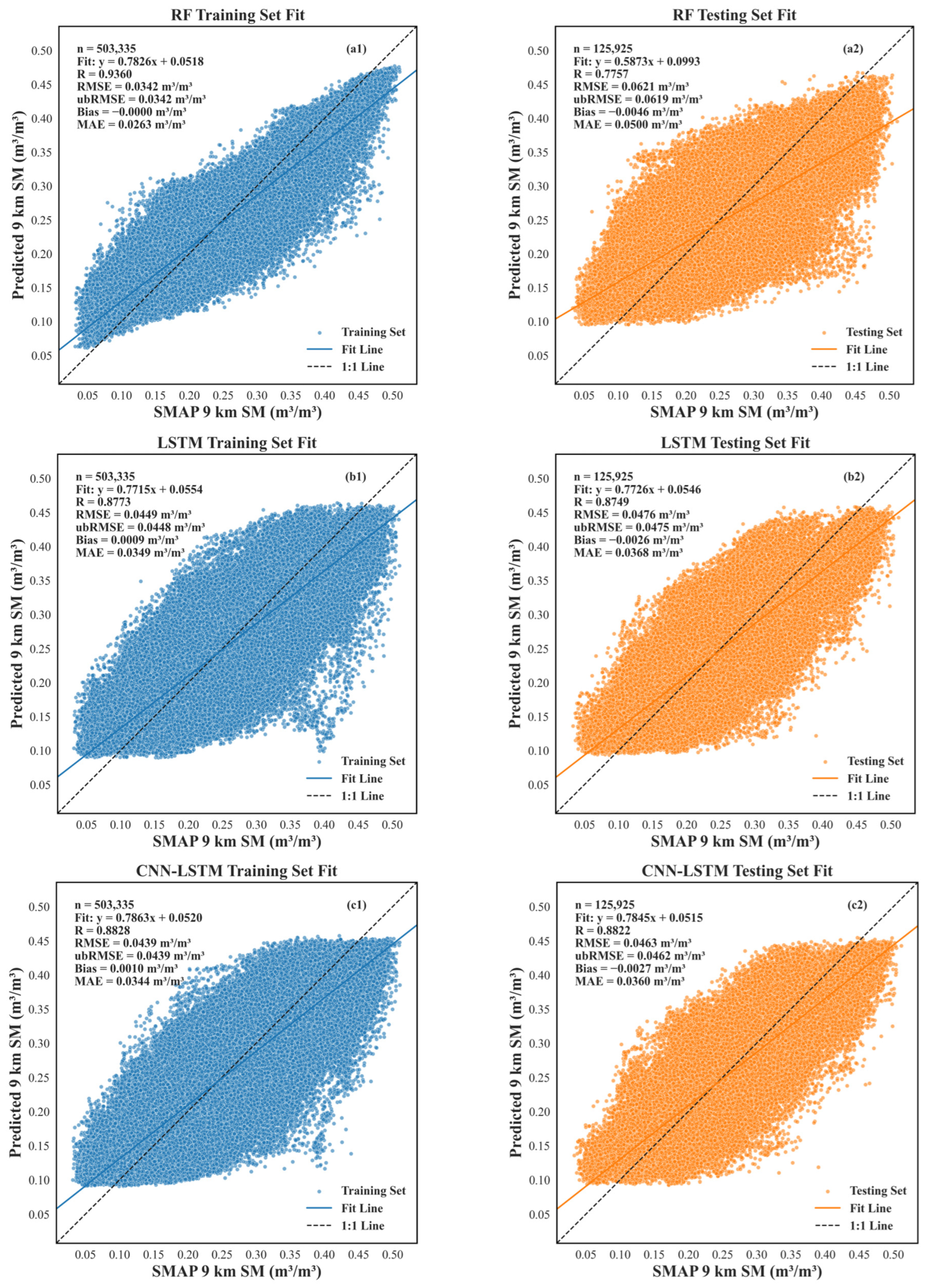
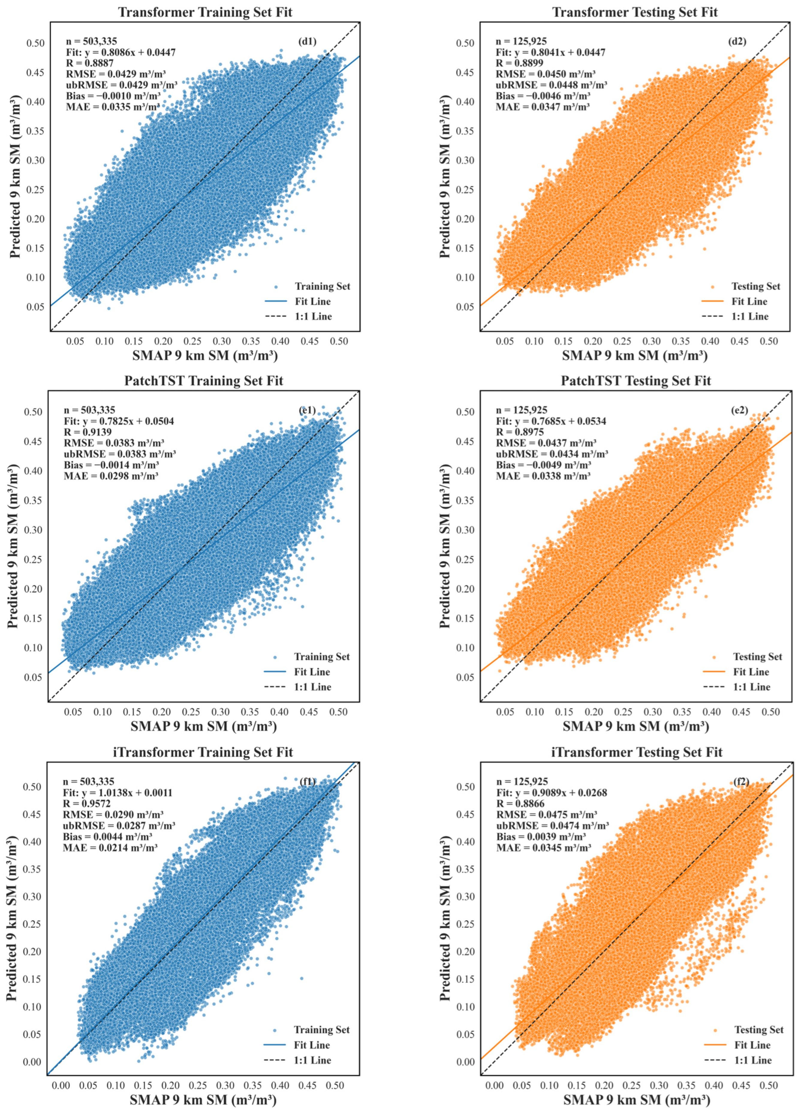
To more intuitively demonstrate the fitting performance of the models on the training and test sets, this study presented regression scatter plots between model predictions and SMAP L4 SM observations, as shown in Figure 4.

The regression relationships between predictions from the RF model and original SMAP L4-SM observations are presented in Figure 4(a1,a2). For the training set of the RF, the slope of the regression line was 0.7826, close to the 1:1 line, and the scatter points were densely distributed, indicating decent fitting performance on training data. On the test set, however, the regression slope dropped to 0.5873, which deviated substantially from 1. The scatter points showed obvious fan-shaped divergence. Particularly in the moderate and high SM ranges (marked by red circles), the predicted values were evidently underestimated, revealing the poor performance of RF on the test set. Although hyperparameter tuning was conducted to mitigate overfitting during model training in Section 3.3.1, RF still failed to effectively capture the complex variations in SM. This finding was consistent with the evaluation metrics above, demonstrating that RF had limitations in fully characterizing the nonlinear relationships between SM and environmental variables, especially for areas with moderate and high SM.

LSTM and CNN-LSTM exhibited similar regression patterns, as shown in Figure 4(b1,b2) and Figure 4(c1,c2). On the test set, the regression slopes of LSTM and CNN-LSTM were 0.7726 and 0.7845, with intercepts of 0.0546 and 0.0515, respectively. Their overall fitting performance was much better than that of RF (slope = 0.5873, intercept = 0.0993). The scatter plots showed that predicted values generally lay above the 1:1 line in the low moisture range (SMAP SM < 0.15 m³/m³), indicating overestimation. In the moderate and high moisture range (SMAP SM > 0.35 m³/m³), predictions mostly fell below the 1:1 line, suggesting underestimation. The results implied that although LSTM and CNN-LSTM achieved stronger generalization than RF, they could not fully respond to the dynamic variation in SM and performed poorly for extreme moisture conditions. Benefiting from the convolutional structure that enhanced the extraction of local temporal features, CNN-LSTM achieved slightly better fitting and more concentrated scatter points than LSTM.

Transformer-based models exhibited distinct advantages in two complementary evaluation dimensions: point prediction accuracy (i.e., RMSE, MAE, and R) and overall trend consistency (i.e., regression slope and intercept). As illustrated in Figure 4(d1,d2), the Transformer model showed uniformly and symmetrically distributed scatter points across the entire moisture range, with a test regression slope of 0.8041 and an intercept of 0.0447, both of which were superior to those of the LSTM-based models and the RF model. Its point prediction accuracy (RMSE = 0.0450 m³/m³, R = 0.8899) was also superior to that of classic models, indicating that the model achieved a well-balanced performance in both dimensions.

As illustrated in Figure 4(e1–f2), PatchTST and iTransformer showed different strengths. PatchTST achieved the highest point prediction accuracy among all models (test RMSE = 0.0437 m³/m³, R = 0.8975), with the most concentrated scatter cloud around the regression line. However, its test regression slope (0.7685) was relatively lower, indicating a conservative response to high moisture values. In contrast, iTransformer exhibited the strongest trend consistency among all models, with the highest test slope (0.9089) and the lowest test intercept (0.0268) among all models, reflecting good agreement between its predictions and observations in terms of the overall variation range. Nevertheless, its scatter cloud showed slightly wider dispersion, consistent with its relatively higher test RMSE (0.0475 m³/m³), which was comparable to that of LSTM (0.0476 m³/m³) and may have been influenced by a limited number of large-error samples. Despite these variant-specific characteristics, all three Transformer-based models outperformed RF in both point prediction accuracy and trend consistency, and at least two of the three variants surpassed the LSTM-based models in each evaluation dimension. This collectively demonstrates that Transformer-based architectures possess flexibility and overall effectiveness in SM downscaling tasks.

Combining quantitative metrics and regression analysis, Transformer-based models outperformed the classic models. They are promising approaches for accurate SM downscaling.

4.2. Validation of Downscaled SM Accuracy

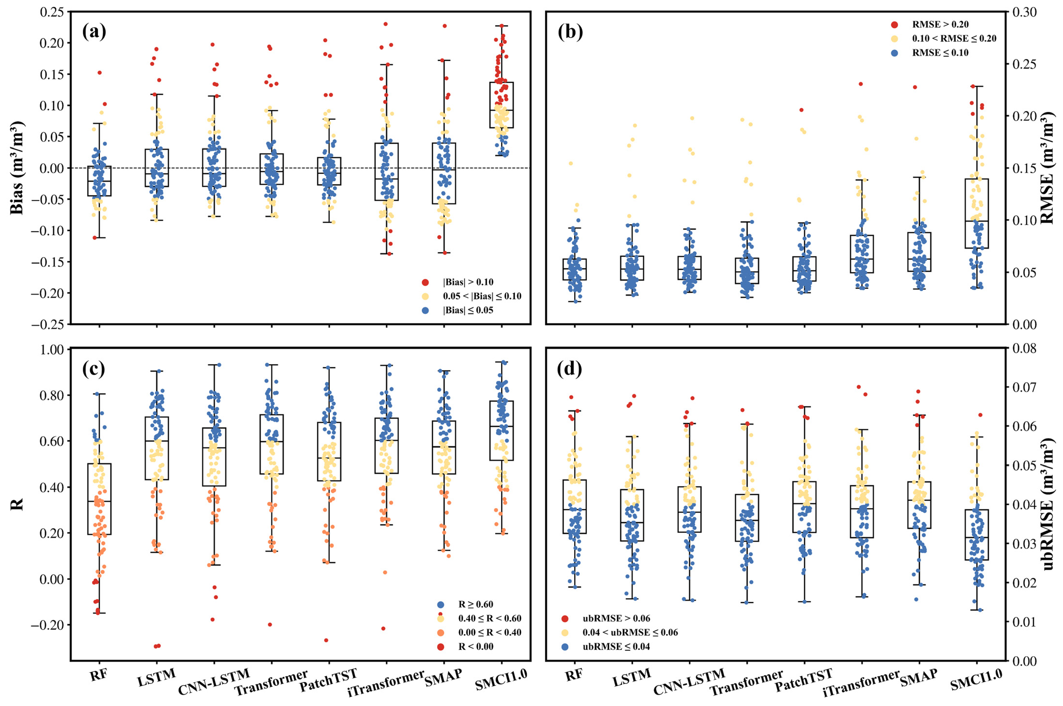
On the basis of the model performance analysis in Section 4.1, high-resolution downscaling factors were input into each model to generate daily 1 km SM products spanning from 1 April 2015 to 31 December 2022. Further accuracy validation for these products was then conducted. Anhui Province features densely distributed in situ observation stations, as shown in Figure 1c. Station measurements serve as a critical reference for validating the accuracy of remotely sensed and model-retrieved SM products [54]. Using in situ SM observations collected in 2019, this study calculated evaluation metrics including R, Bias, RMSE, and ubRMSE for 87 stations across the study area. Note that the 10 cm in situ SM observations used for validation were selected as the closest available near-surface measurements to SMAP L4-SM (0–5 cm). Comparisons were made between field measurements and eight SM products, including the original SMAP L4-SM product, the publicly available 1 km SMCI1.0 SM product, and six downscaled SM products generated by different models. The results are presented in Figure 5. Observation frequency varied across individual stations. Directly combining all data for integrated evaluation would cause stations with more records to dominate the overall results, mask the accuracy performance at other sites, and introduce statistical Bias. Accordingly, this study adopted a station-averaging method: evaluation metrics were first calculated for each station separately and then averaged. This approach assigns equal weight to all stations and objectively reflects the overall accuracy of different SM products over the entire study area. The averaged metric values are summarized in

Table 3. Overall accuracy evaluation of each SM product based on 87 in situ observation stations.

Products	Mean Bias (m3/m3)	Mean Absolute Bias (m3/m3)	Mean R	Mean ubRMSE (m3/m3)	Mean RMSE (m3/m3)
SMAP L4-SM	−0.0023	0.0531	0.5515	0.0407	0.0719
SMCI1.0 SM	0.1018	0.1018	0.6358	0.0331	0.1088
RF Downscaled SM	−0.0174	0.0340	0.3336	0.0395	0.0562
LSTM Downscaled SM	0.0068	0.0403	0.5402	0.0374	0.0599
CNN-LSTM Downscaled SM	0.0059	0.0397	0.5259	0.0391	0.0607
Transformer Downscaled SM	0.0055	0.0382	0.5617	0.0372	0.0591
PatchTST Downscaled SM	0.0042	0.0364	0.5305	0.0401	0.0597
iTransformer Downscaled SM	0.0003	0.0577	0.5624	0.0390	0.0751

.

Combining Figure 5 and Table 3, the downscaled SM products showed clear differences in validation accuracy. The RF-downscaled SM showed relatively poor consistency with in situ observations, with the lowest average R (0.3336), indicating limited capability in reproducing temporal SM variations. The LSTM and CNN-LSTM-based products exhibited improved performance compared with RF, but their overall performance remained inferior to that of the Transformer-based products. PatchTST showed good Bias control among the Transformer-based products, with the lowest mean absolute Bias (0.0364 m³/m³) among the three Transformer-based downscaled products. Nevertheless, its average R (0.5305) was lower than that of Transformer and iTransformer, suggesting weaker capability to capture temporal SM dynamics, and its ubRMSE (0.0401 m³/m³) and RMSE (0.0597 m³/m³) were also relatively higher than Transformer. iTransformer showed the highest average R (0.5624) among the six downscaled products and the Bias closest to zero (0.0003 m³/m³), indicating excellent overall trend consistency and no systematic deviation. However, its mean absolute Bias (0.0577 m³/m³) and RMSE (0.0751 m³/m³) were the highest among the downscaled products, consistent with the findings in Section 4.1 that iTransformer’s performance was influenced by a limited number of large-error samples.

Specifically, Transformer did not rank first in every single metric, but presented the most balanced performance. It obtained the lowest average ubRMSE and the second-highest average R among all six downscaled SM products, demonstrating its superior ability and accuracy in capturing actual SM variations. Its mean absolute Bias of 0.0382 m³/m³ and average RMSE of 0.0591 m³/m³ remained at relatively low levels and were substantially better than those of the publicly available SMCI1.0 SM product, as also illustrated in the metric distribution plots in Figure 5. Notably, Transformer successfully downscaled the original 9 km SMAP L4-SM product to 1 km resolution while maintaining and even improving accuracy. Its average ubRMSE (0.0372 m³/m³), RMSE (0.0591 m³/m³), and R (0.5617) all outperformed those of SMAP L4-SM, reflecting remarkable stability in accuracy. In contrast, the SMCI1.0 SM product had the poorest accuracy. This product was developed using data from 1648 in situ stations across China, including the 87 stations in Anhui Province used for validation in this study. Therefore, the relatively high average R (0.6358) of SMCI1.0 should be interpreted with caution, as the shared station observations may have partially influenced its correlation performance. Nevertheless, SMCI1.0 exhibited a large systematic overestimation (Bias = 0.1018 m³/m³) and the highest RMSE (0.1088 m³/m³) among the evaluated products, which were substantially worse than those of the Transformer-downscaled product. This indicates that, despite the potential influence of shared observations, the Transformer-downscaled product demonstrated superior overall accuracy based on comprehensive evaluation metrics. Therefore, the Transformer-downscaled product was selected for the subsequent analyses.

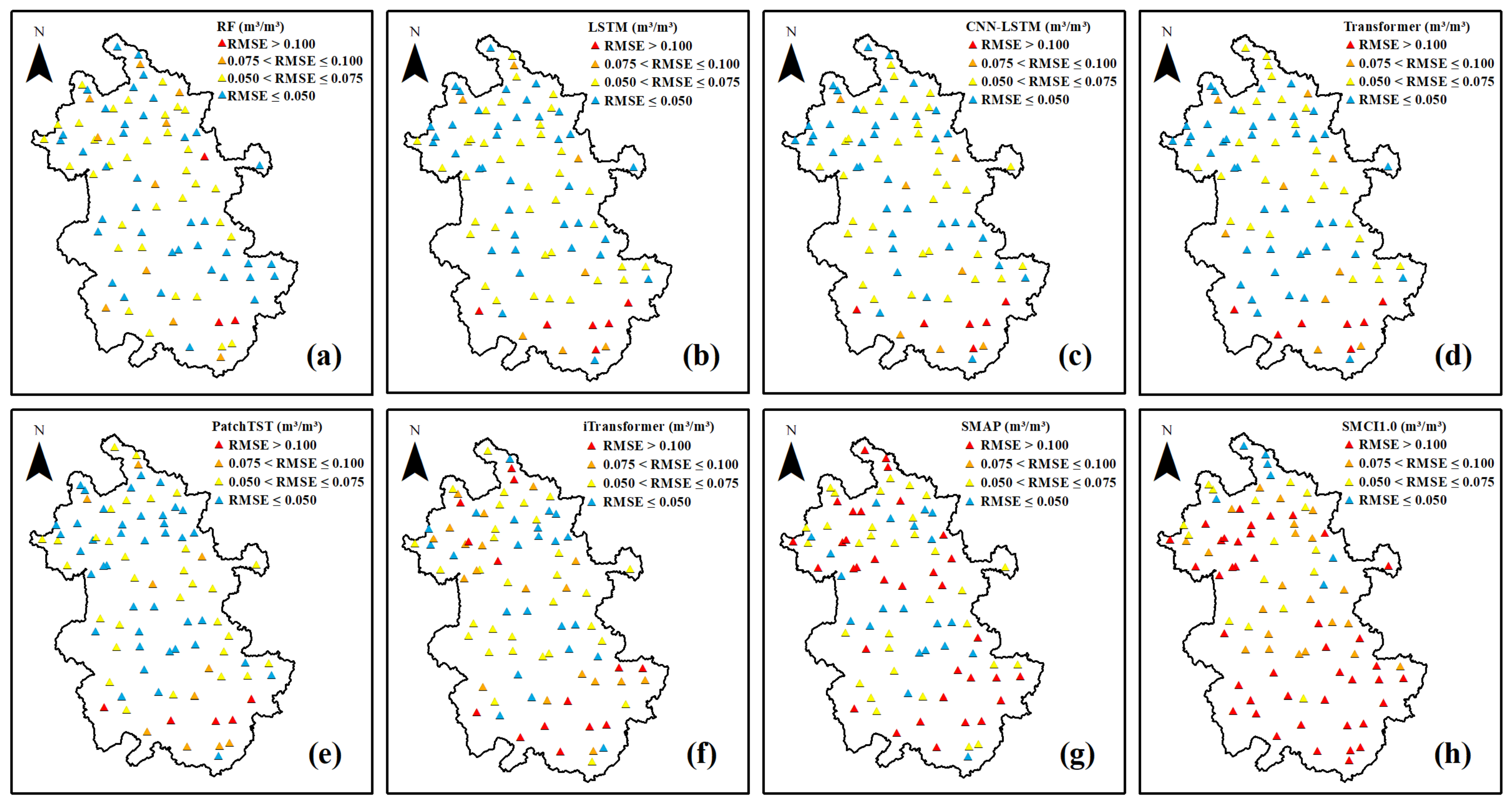
To further investigate the spatial variability of model performance across the study area, station-level RMSE values for each product were spatially mapped, as shown in Figure 6. Overall, all products exhibited evident spatial heterogeneity. High-RMSE stations (RMSE > 0.075 m³/m³) were relatively concentrated in the southern part of Anhui Province, while low-RMSE stations (RMSE ≤ 0.050 m³/m³) were more frequently observed in the central and northern areas. This spatial pattern may be attributed to regional differences in land cover and topography across Anhui Province. Among the six downscaled products, Transformer and PatchTST showed a higher proportion of low-RMSE stations, indicating more stable spatial performance. Although PatchTST also exhibited good spatial stability, its lower average R (0.5305) and higher ubRMSE (0.0401 m³/m³), as shown in Table 3, resulted in a less balanced overall performance compared with the Transformer product. iTransformer exhibited a noticeably larger number of high-RMSE stations, particularly in the northern part of the province, consistent with its higher average RMSE shown in Table 3. The original SMAP L4-SM and SMCI1.0 products showed the most extensive high-RMSE areas, further confirming the effectiveness of the downscaling approach. These station-level spatial results are consistent with the averaged metrics in Figure 5 and Table 3, while additionally revealing regional differences that cannot be captured by average statistics alone.

In summary, the accuracy assessment based on in situ station data proves that the Transformer-based downscaled SM product established in this study achieved an optimal balance between spatial resolution and accuracy. It not only improved the spatial resolution of the original SMAP L4-SM product from 9 km to 1 km to meet the demand for high-resolution data in regional hydrological applications, but also outperformed the original product, downscaled products from comparative models, and the existing 1 km SMCI1.0 SM product in overall accuracy. The results further verify the effectiveness and reliability of the Transformer model for SM downscaling.

4.3. Spatial Distribution of Downscaled SM in Anhui

The accuracy of the Transformer-based downscaled SM product was systematically verified in Section 4.2, confirming its reliability. To further evaluate whether the downscaled product preserved the spatial patterns and temporal variations in the original SMAP observations while providing enhanced spatial detail, quantitative correlation analyses and representative spatial comparisons were performed. We generated continuous daily downscaled SM products from 1 April 2015 to 31 December 2022. Given the consistent spatial patterns across years, presenting daily results for each year would produce excessive figures. Since SM exhibited prominent fluctuations in 2019, which well reflected the intra-annual spatiotemporal dynamics of SM over Anhui Province, this year was selected as a typical case to compare spatial distributions and seasonal characteristics between the original and downscaled SM products.

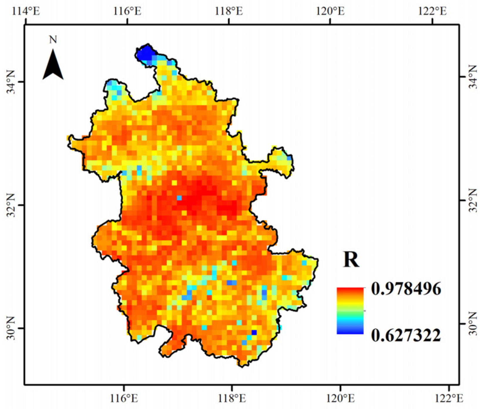
To further evaluate the consistency of temporal variations between the original and downscaled SM products, pixel-wise temporal correlation analysis was performed using daily SM time series from April 2015 to December 2022. The 1 km downscaled SM product was aggregated to the original 9 km SMAP grid, and R was calculated between the two products for each grid cell. The spatial distribution of the pixel-wise R is shown in Figure 7. R was high across Anhui Province, with a provincial mean of 0.9315 and 99.30% of pixels exceeding 0.8, indicating that the Transformer-based downscaled SM product effectively preserved the temporal dynamics of the original SMAP observations across different regions. Relatively lower correlations were observed in the mountainous areas of southern Anhui, likely due to the complex terrain and environmental conditions.

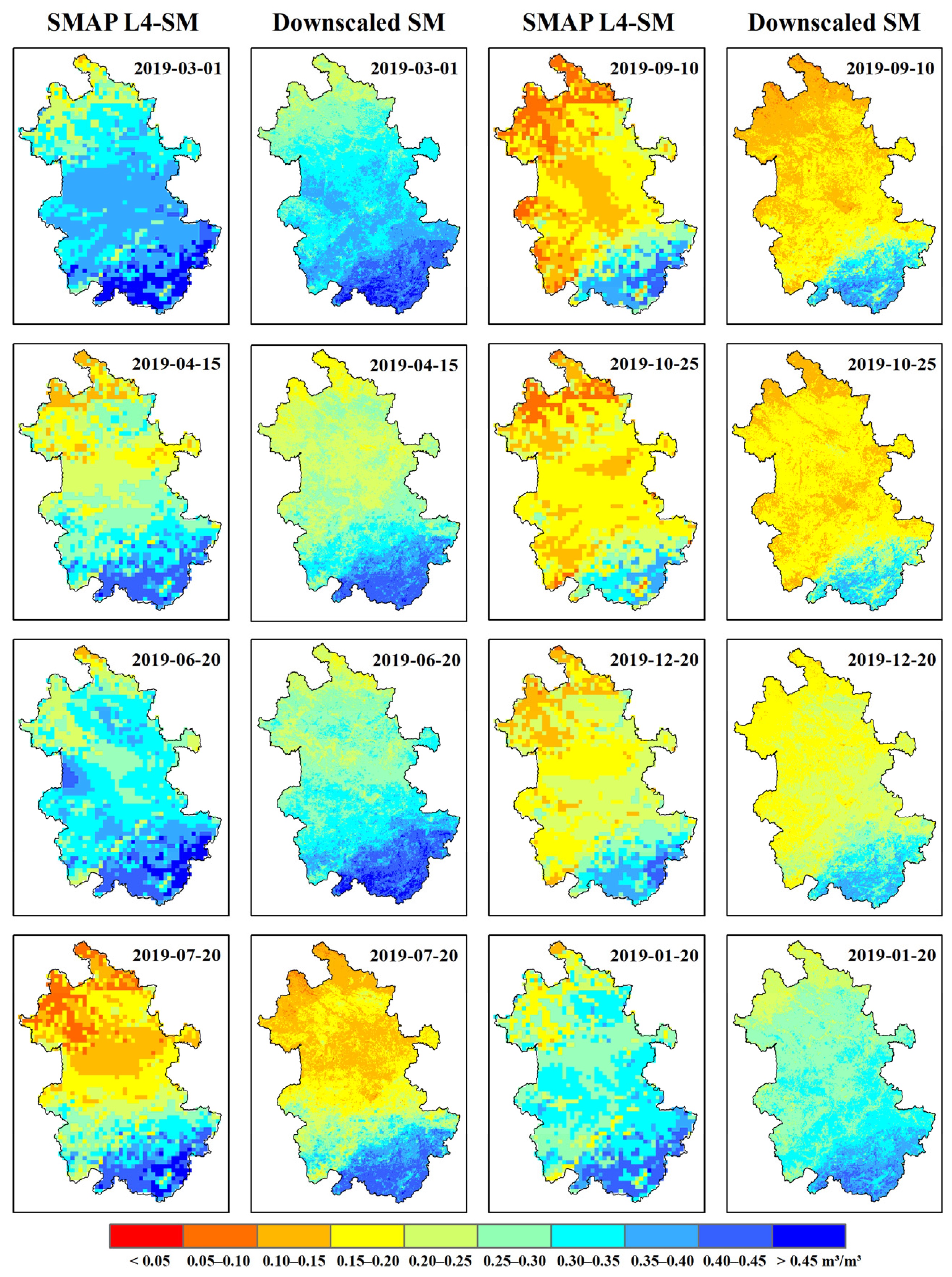
In addition to the long-term temporal consistency assessment, the spatial pattern consistency between the original and downscaled SM products was further evaluated using representative dates in 2019. Eight representative dates were selected to cover different seasonal conditions, including March 1 and April 15 in spring, June 20 and July 20 in summer, September 10 and October 25 in autumn, and December 20 and January 20 in winter. As summarized in

Table 4. Spatial R between SMAP and Transformer-downscaled SM products for representative dates in 2019.

Date	p-Value	Spatial-R
2019-01-20	1.84102 × 10−204	0.6463
2019-03-01	6.6864 × 10−291	0.7334
2019-04-15	0.0000	0.7836
2019-06-20	2.41791 × 10−231	0.6768
2019-07-20	0.0000	0.8957
2019-09-10	0.0000	0.8254
2019-10-25	3.12217 × 10−289	0.7319
2019-12-20	0.0000	0.7892

, the spatial R ranged from 0.6463 (January 20) to 0.8957 (July 20), with an average value of 0.7603 across all selected dates (all p < 0.001). The consistently high correlations indicate that the Transformer-based downscaled SM product effectively retained the spatial distribution patterns of the original SMAP observations.

Although the quantitative spatial correlation analysis confirmed the consistency of both temporal dynamics and spatial patterns between the two products, visual comparisons were further conducted to examine the spatial refinement capability of the downscaled product. The spatial distribution of SM before and after downscaling is shown in Figure 8. Both the original and downscaled SM products clearly exhibited typical seasonal dynamics. The downscaled SM not only retained the spatial distribution characteristics of the original SM product but also provided finer spatial details. Moreover, SM in southern Anhui remained above 0.3 m³/m³ throughout most of the year with relatively stable variations. Based on Figure 1b,c, this phenomenon can be attributed to the mountainous terrain, high forest coverage, and strong evapotranspiration regulation in the southern region. Therefore, SM in this area remained at a relatively high level year-round with limited seasonal variation, showing continuous and stable spatial distribution.

At the seasonal scale, the downscaled product captured the key spatiotemporal transitions of SM across Anhui Province. In spring, SM was generally high in early March due to snowmelt and seasonal precipitation, with southern mountainous areas wetter than the central and northern plains; by mid-April, rising temperatures and enhanced evapotranspiration caused a pronounced SM decline, particularly in cropland areas. In summer, frequent plum rain precipitation in late June led to relatively balanced SM across the province, whereas the hot and dry conditions after mid-July intensified the north–south contrast as southern forests retained more moisture than northern farmland. In autumn, reduced precipitation and persistent evapotranspiration during crop maturation lowered regional SM in early September, and crop harvesting by late October further smoothed the spatial distribution. In winter, SM gradually recovered with declining temperatures and accumulated precipitation in December; by mid-January, low temperatures and snowfall stabilized SM and narrowed regional discrepancies. Across all seasons, the downscaled product consistently revealed more detailed spatial heterogeneity in localized wet and dry transitions and land-cover boundaries compared with the original 9 km product.

In summary, the quantitative correlation analyses confirm that the downscaled product preserves both the temporal dynamics (mean pixel-wise R = 0.9315) and spatial patterns (mean spatial R = 0.7603) of the original SMAP product. Building on this consistency, the 1 km downscaled SM reveals substantially richer spatial details, particularly in localized wet and dry regions, land-cover boundaries, and topographic transitions, while maintaining reasonable seasonal variations. These results further validate the reliability of the downscaled SM product derived from the Transformer model.

4.4. Precipitation Response Characteristics of Downscaled SM

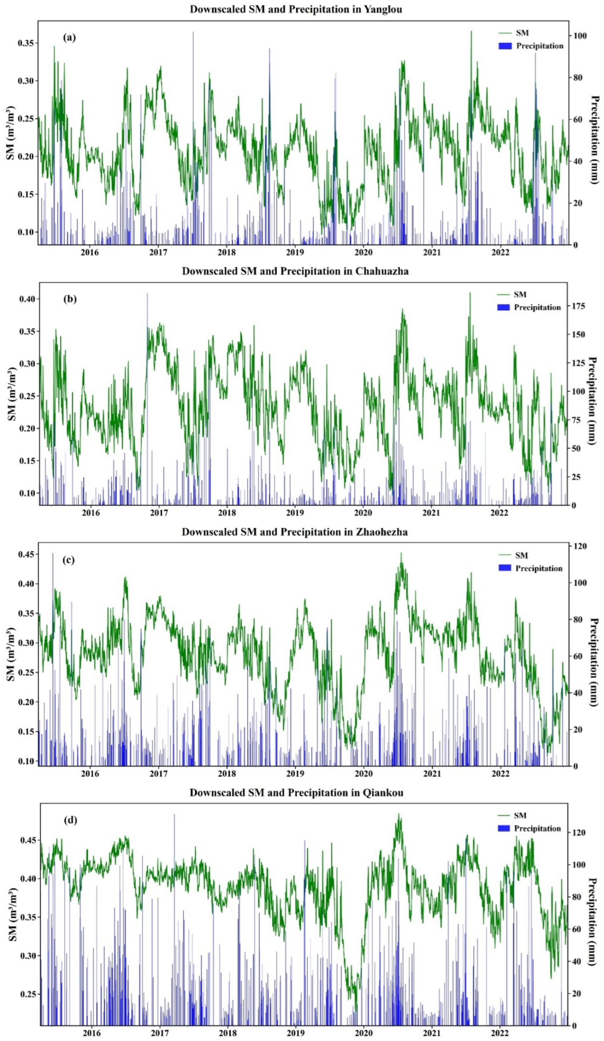
In SM downscaling research, precipitation acts not only as an important input and key feature variable for model construction that affects the spatiotemporal distribution of SM, but also serves as an independent reference variable to analyze how downscaled SM products respond to precipitation events. To further explore such responses, this study selected four representative in situ stations across different regions of Anhui Province: Yanglou in the northernmost area, Chahuazha in the north-central area, Zhaohezha in the south-central area, and Qiankou in the southern area. We extracted precipitation and Transformer-based downscaled SM time series data for these stations from 2015 to 2022 and conducted comparative analysis via time series plots. The locations of the four stations are presented in Figure 1c, and their time series of precipitation and downscaled SM are shown in Figure 9.

Overall, the temporal variations at the four stations indicate that the downscaled SM product generally captures precipitation-driven fluctuations across different climatic and environmental conditions in Anhui Province. During periods with frequent or intense precipitation, SM exhibited clear increasing trends, whereas prolonged precipitation deficits corresponded to sustained SM decreases. For example, during the plum rain season in mid-2020, persistent heavy rainfall across Anhui Province resulted in substantial SM increases at all four stations, with Zhaohezha and Qiankou reaching approximately 0.45 m³/m³. In contrast, during the relatively dry years of 2019 and 2022, reduced precipitation was accompanied by persistent SM decreases, particularly at the agricultural stations Yanglou, Chahuazha, and Zhaohezha, where minimum values approached 0.10 m³/m³. At Qiankou, however, the minimum SM remained around 0.25 m³/m³, owing to the strong regulatory capacity of forest vegetation in the southern mountainous area. Occasionally, SM rose during low-precipitation periods, which can be attributed to antecedent precipitation accumulation, winter snowmelt, and agricultural irrigation at cropland stations such as Chahuazha.

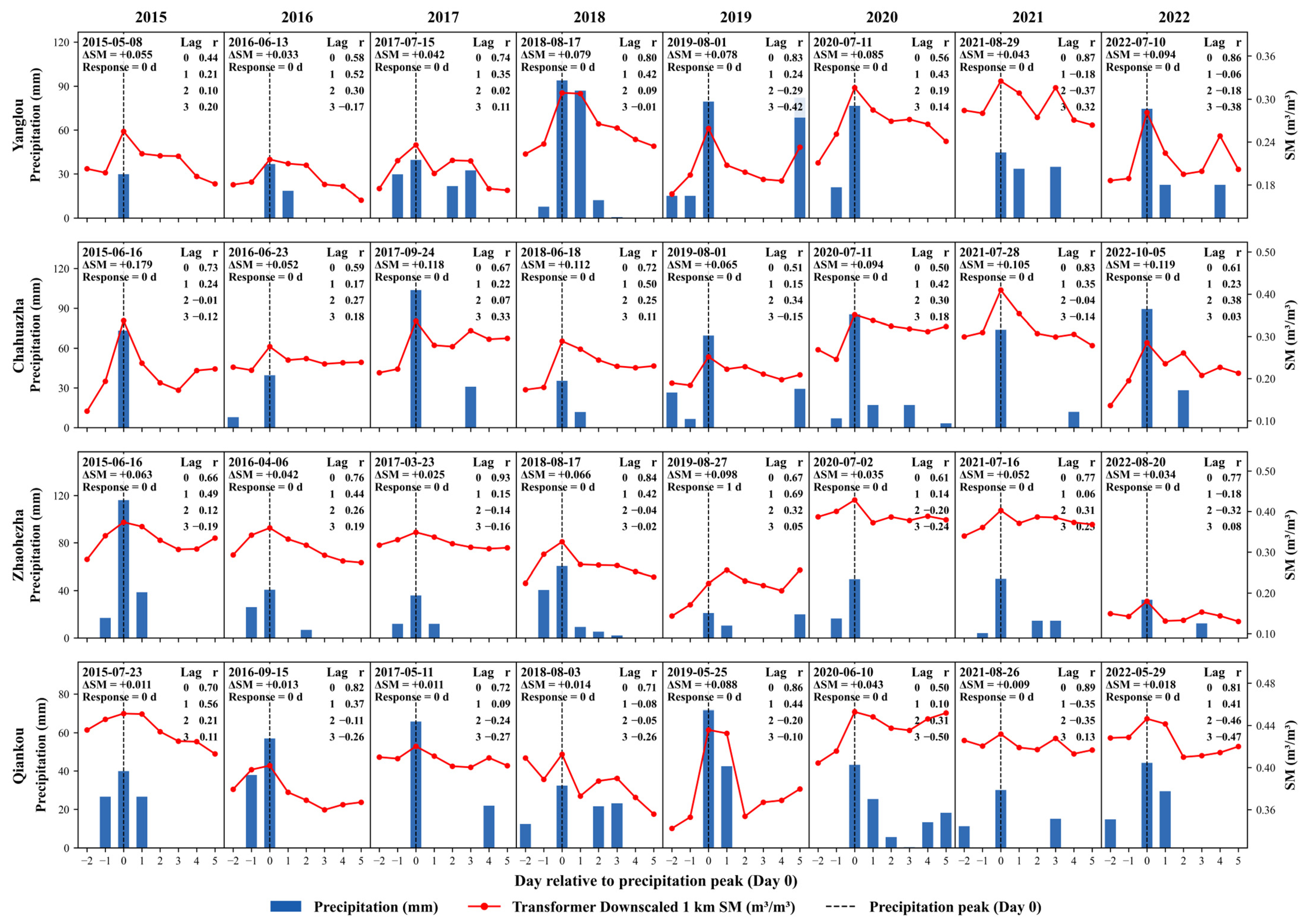
Although Figure 9 demonstrates the overall consistency between precipitation and SM variations at interannual and seasonal scales, the detailed response characteristics of SM following individual precipitation events require further quantitative evaluation. Therefore, for each station and year from 2015 to 2022, one representative precipitation event was selected, requiring at least two consecutive rain-free days before and after the event to isolate its effect. In total, 32 events were analyzed. For each event, the day of maximum precipitation was defined as Day 0, and the SM evolution within a window from Day −2 to Day +5 was extracted. The precipitation-driven SM responses, including the response magnitude (ΔSM), peak timing (response), and lagged correlations (r), are summarized in Figure 10.

As shown in Figure 10, the downscaled SM exhibits a rapid and consistent response to all selected precipitation events. In nearly every event, the SM curve rises sharply on Day 0 and reaches its peak on the same day, as indicated by the response value of 0 d in most panels; only one event at Zhaohezha in 2019 shows a one-day Lag. The lagged correlation coefficients in the upper-right corner of each panel further confirm this synchrony: the Lag-0 coefficient is consistently positive and relatively high across stations and years, whereas the coefficients at Lag 1 are markedly lower, and those at Lag 2 and Lag 3 are close to zero or become negative. This pattern indicates that the downscaled product effectively captures rapid SM adjustments associated with precipitation events, and that the influence of a single precipitation event decays rapidly within two to three days.

Figure 10 also reveals the spatial differences in SM response magnitude to precipitation events. The ΔSM values are generally larger at the northern and central stations (Yanglou, Chahuazha, and Zhaohezha) than at the southern station Qiankou. At Qiankou, the SM curve remains at a high absolute level throughout the event window, reflecting a high pre-event SM level conditioned by the humid mountainous climate and dense forest cover in southern Anhui; consequently, the additional increment caused by an individual precipitation event is comparatively small. In contrast, at the northern or central stations, the pre-event SM level is generally lower, leaving more room for SM to rise after precipitation and resulting in a more pronounced increment. Despite these spatial differences in response amplitude, the downscaled SM product consistently captures the precipitation-driven SM dynamics across all four stations.

Overall, both the long-term time series (Figure 9) and the quantitative analysis of 32 representative precipitation events (Figure 10) demonstrate that the Transformer- downscaled 1 km SM product exhibits a strong and consistent response to precipitation. During rainfall events, SM rises rapidly and typically peaks on the same day, with high Lag-zero correlations that decay within two to three days. These results confirm that the Transformer-based downscaling framework reliably captures precipitation-driven SM dynamics, underscoring the robust precipitation response capability of the downscaled product.

5. Discussion

5.1. Analysis of Influencing Factor Importance

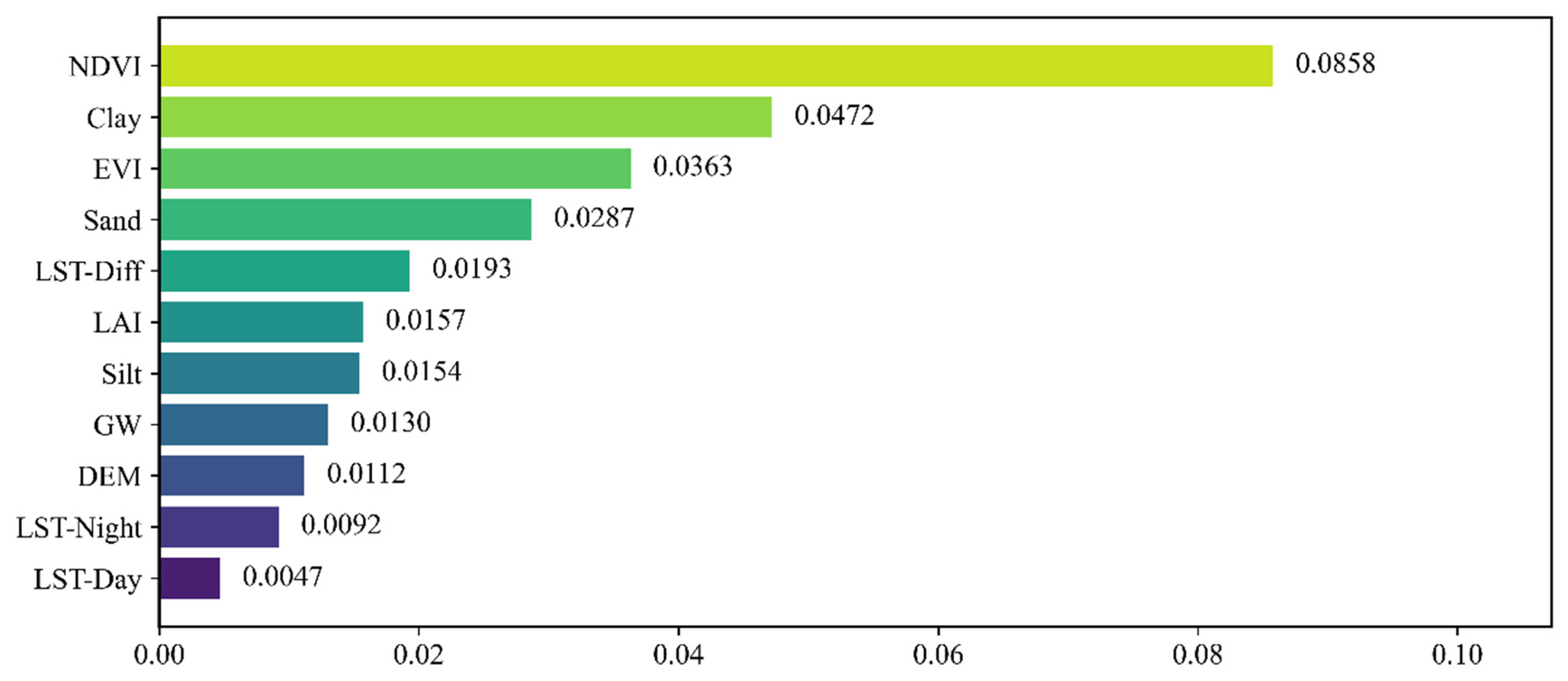
In the selection of downscaling factors, this study incorporated a more comprehensive water transfer mechanism. In addition to commonly used influencing factors (such as vegetation indices, precipitation, and topography), deeper hydro-meteorological coupling factors like LST-Diff and GW were also introduced. This section presents an importance analysis of the influencing factors used in the study. The Permutation Feature Importance (PFI) method was employed based on the Transformer model to quantitatively assess the contribution of each input factor to the model predictions, aiming to reveal the impact of different variables on the SM prediction results.

Due to the overwhelming importance of the precipitation factor in modeling, this study focused on presenting the contribution rankings of the remaining influencing factors to avoid its dominance from masking the performance of other variables. The results of the feature importance analysis are shown in Figure 11. According to the results, vegetation index features (such as NDVI, EVI, and LAI) played a significant role in SM downscaling modeling, among which NDVI had the highest importance (0.0858), indicating that surface vegetation coverage played a key role in characterizing the spatial distribution of SM. This result was consistent with previous studies [27]. In addition, soil texture features also exhibited a strong influence. For example, Clay (0.0472), Sand (0.0287), and Silt (0.0154) all contributed to SM prediction to a certain extent. Different soil textures determined the water-holding capacity and permeability of the soil, thereby affecting the spatial distribution and dynamic changes in SM [55]. This result reflected that the introduction of static geological variables was of great significance for characterizing the spatial heterogeneity of SM.

LST-Diff and GW were introduced as coupling factors reflecting deeper hydro-meteorological processes, and they demonstrated importance in SM downscaling second only to vegetation indices and soil texture. LST-Diff can indirectly reflect the dynamic variation in SM, as moist soils have higher heat capacity than dry soils [56,57], resulting in smaller diurnal temperature fluctuations [9]. The influence of LST-Diff (0.0193) on SM prediction was significantly stronger than that of LST-Night (0.0092) and LST-Day (0.0047), indicating that it played a more important role in SM downscaling modeling. The influence of GW (0.0130) reflected the potential recharge capacity of deep SM to surface SM, and GW showed slightly higher importance than DEM. This was consistent with previous findings: since GW plays a significant regulatory role in SM and regional water cycle processes, spatial differences in groundwater depth may lead to pronounced spatial heterogeneity in SM and surface moisture fluxes at the regional scale. Especially in areas with shallow groundwater tables, its influence on SM and surface evaporation can be comparable to the variability caused by topography and land cover [58].

Although DEM is generally considered an important factor influencing SM dynamics, it showed a relatively low feature importance of 0.0112. Previous research has indicated that in SM downscaling modeling based on terrain partitioning, DEM often exhibits higher feature importance than vegetation index factors. However, this study adopted a unified modeling strategy for the entire province, and as a static topographic variable, the local elevation differences in DEM were difficult to exert a significant influence on the overall modeling. It should be noted that the PFI-based feature importance can be influenced by correlations among input variables. Therefore, the importance rankings should be interpreted as the relative importance of variables within the current feature set. Future studies could further combine complementary explainable methods, such as SHAP, to provide a more comprehensive understanding of feature importance.

5.2. Limitations of This Study

In this study, the Transformer-based SM downscaling product achieved good accuracy, but there are still certain uncertainties in data, methodology, and result validation that need to be discussed and explained.

The accuracy of the downscaled SM product obtained was limited by the original 9 km SMAP L4-SM data. As observed in Table 3 and Figure 5, there were errors between the original SMAP data and the in situ measurements, with an average ubRMSE of 0.0407 m³/m³. The average ubRMSE of the downscaled SM was reduced to 0.0372 m³/m³ due to the influence of multi-source auxiliary variables. However, the original SMAP L4-SM, serving as the supervisory variable, inherently limited the potential accuracy improvement of the final product. Future work may consider incorporating multi-source remote sensing SM products to alleviate the constraints imposed by errors from a single data source on the accuracy of downscaled SM products.

During the preprocessing of downscaling factors, to improve the completeness and continuity of multi-source time series feature data, some variables (such as NDVI, EVI, LAI, and GW) were processed using S-G filtering and interpolation methods to fill missing values or smooth anomalies. Although this approach alleviated the impact of data gaps to some extent, it might also introduce estimation errors, especially during periods with high data variability. Such errors may weaken the original temporal characteristics of the variables and affect the model’s depiction of SM dynamics. Future studies could adopt machine learning-based time series interpolation or multi-source data fusion strategies to further enhance the authenticity of input features, thereby improving the accuracy and reliability of downscaled SM products.

In the validation of the downscaled SM products, accuracy assessment mainly relied on in situ station SM data, but discrepancies still existed in spatial and depth matching [50]. The original SMAP product represents SM at 0–5 cm depth, while the in situ stations provide measurements at 10 cm depth. Although previous studies have demonstrated strong correlations between adjacent soil layers [59], the depth-related differences cannot be ignored. Additionally, using the average SM value within a 1 km grid to represent a single-point observation from a station might introduce errors caused by spatial scale mismatch. Introducing higher-resolution downscaling factors to achieve finer-resolution SM products (e.g., 30 m) could significantly reduce spatial matching errors and improve the reliability of accuracy validation.

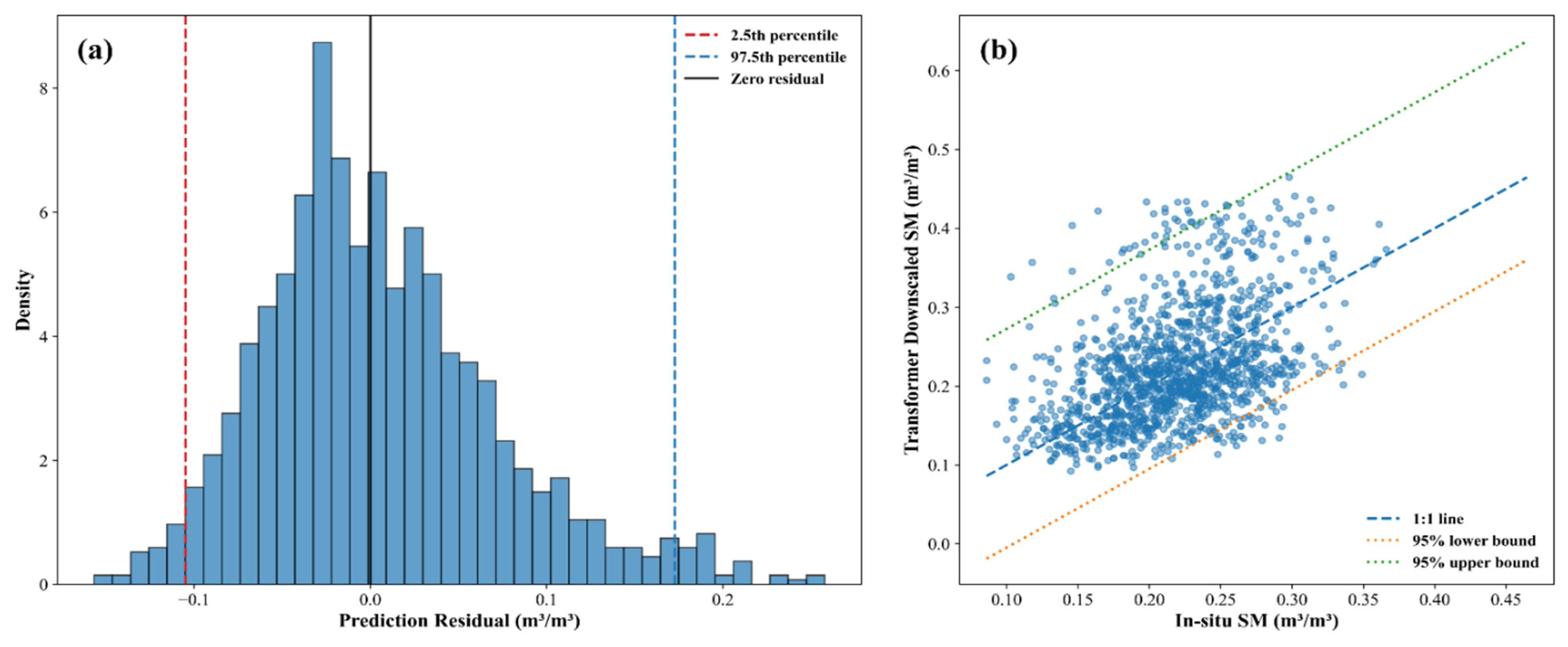
To further quantify the prediction uncertainty, the residuals between the Transformer-downscaled SM and the in situ observations were analyzed, as shown in Figure 12 and

Table 5. Quantitative results of prediction uncertainty analysis for the Transformer-downscaled SM product.

Metric	Value
Number of stations	87
Mean residual (m3/m3)	0.0052
Median residual (m3/m3)	−0.0045
2.5th residual percentile (m3/m3)	−0.1049
97.5th residual percentile (m3/m3)	0.1727
Prediction interval coverage (%)	94.8916
Nominal prediction interval coverage (%)	95

. The 2.5th and 97.5th percentiles of the residuals were −0.1049 m³/m³ and 0.1727 m³/m³, respectively, corresponding to an empirical 95% prediction interval. Furthermore, each date was treated as a held-out validation date, with the prediction interval estimated from the residuals of the remaining dates and its coverage evaluated using the observations on the held-out date. The overall coverage was 94.8916%, close to the nominal 95% level. Overall, these results indicate that although uncertainties associated with the supervisory data, input data preprocessing, and spatial and depth mismatches remain, the prediction-error uncertainty of the downscaled SM product can be reasonably characterized, and the product still demonstrates a satisfactory level of reliability in the presence of these uncertainties.

In addition, the applicability of the proposed framework beyond Anhui Province requires further evaluation. Although the Transformer-based model achieved satisfactory performance within the study region, the relationships between SM and auxiliary environmental variables may differ under other climatic and geomorphological conditions. For example, the relative importance of groundwater, precipitation, and soil properties may vary across regions due to differences in climate and land surface characteristics. Direct application to new regions may therefore require regional adaptation and further validation. Temporal-split validation such as leave-one-year-out experiments can also be adopted to fully characterize the temporal generalization of downscaling models.

6. Conclusions

To meet the demand for high-resolution SM products, this study established an SM downscaling framework integrating multi-source features based on the Transformer algorithm, taking Anhui Province with complex landforms as the study area, and generated a high-precision 1 km daily SM dataset covering 2015 to 2022. The main conclusions are summarized as follows:

(1) Compared with classic models including RF, LSTM, and CNN-LSTM, Transformer and its variants overall demonstrated superior prediction performance and generalization capability. In terms of quantitative evaluation metrics, Transformer-based models achieved good prediction accuracy on the test set, with Transformer (RMSE = 0.0450 m³/m³) and PatchTST (RMSE = 0.0437 m³/m³) obtaining relatively low RMSE values. In terms of regression analysis, Transformer (regression slope = 0.8041) and iTransformer (regression slope = 0.9089) exhibited relatively high prediction trend consistency. Combining quantitative metrics and regression analysis, Transformer and its variants outperform the classic models in characterizing SM variation patterns.

(2) The 1 km downscaled SM product derived from the Transformer model exhibits high accuracy and reliability. Evaluations against in situ SM measurements and the SMCI1.0 product reveal that this downscaled dataset achieves the best overall performance, with a mean ubRMSE = 0.0372 m³/m³ and RMSE = 0.0591 m³/m³. Analysis of its spatial distribution and seasonal variations shows that the product preserves the spatial heterogeneity of the original SMAP SM data and delivers more detailed spatial information. It can also reasonably reflect climatic anomalies across seasons and years. Time series analysis at typical stations further confirms that the downscaled SM responds effectively to precipitation variations.

(3) The introduced LST-Diff and GW factors play vital roles in SM downscaling. Feature importance analysis reveals that these coupled factors reflecting deep hydrometeorological processes rank second only to vegetation indices and soil texture in importance for SM downscaling. In particular, LST-Diff exerts a stronger influence on downscaling performance than conventional daytime and nighttime LST, while GW is more important than DEM. Accordingly, future SM downscaling studies are recommended to adopt LST-Diff instead of separate daytime or nighttime LST, and incorporate deep hydrological factors such as GW to achieve better downscaling results.

Overall, the Transformer-based downscaling framework proposed in this study outperforms classic models including RF, LSTM, and CNN-LSTM in accuracy. The resulting 1 km downscaled SM product also achieves higher precision than the existing 1 km SM product, SMCI1.0. Furthermore, this study presents a feasible approach for SM downscaling by integrating remote sensing data and deep hydrological information, and provides technical support for dynamic monitoring of high-resolution SM at the regional scale.

References

1. Peng, J.; Loew, A.; Merlin, O.; Verhoest, N.E.C. A review of spatial downscaling of satellite remotely sensed soil moisture. Rev. Geophys. 2017, 55, 341–366. [Google Scholar] [CrossRef] [Scilit]
2. Ochsner, T.E.; Cosh, M.H.; Cuenca, R.H.; Dorigo, W.A.; Draper, C.S.; Hagimoto, Y.; Kerr, Y.H.; Larson, K.M.; Njoku, E.G.; Small, E.E.; et al. State of the Art in Large-Scale Soil Moisture Monitoring. Soil Sci. Soc. Am. J. 2013, 77, 1888–1919. [Google Scholar] [CrossRef] [Scilit]
3. Dobriyal, P.; Qureshi, A.; Badola, R.; Hussain, S.A. A review of the methods available for estimating soil moisture and its implications for water resource management. J. Hydrol. 2012, 458–459, 110–117. [Google Scholar] [CrossRef] [Scilit]
4. Bastiaanssen, W.G.M.; Molden, D.J.; Makin, I.W. Remote sensing for irrigated agriculture: Examples from research and possible applications. Agric. Water Manag. 2000, 46, 137–155. [Google Scholar] [CrossRef] [Scilit]
5. Xu, J.; Su, Q.; Li, X.; Ma, J.; Song, W.; Zhang, L.; Su, X. A Spatial Downscaling Framework for SMAP Soil Moisture Based on Stacking Strategy. Remote Sens. 2024, 16, 200. [Google Scholar] [CrossRef] [Scilit]
6. Yan, H.; Zarekarizi, M.; Moradkhani, H. Toward improving drought monitoring using the remotely sensed soil moisture assimilation: A parallel particle filtering framework. Remote Sens. Environ. 2018, 216, 456–471. [Google Scholar] [CrossRef] [Scilit]
7. Seneviratne, S.I.; Corti, T.; Davin, E.L.; Hirschi, M.; Jaeger, E.B.; Lehner, I.; Orlowsky, B.; Teuling, A.J. Investigating soil moisture–climate interactions in a changing climate: A review. Earth–Sci. Rev. 2010, 99, 125–161. [Google Scholar] [CrossRef] [Scilit]
8. Robock, A.; Vinnikov, K.Y.; Srinivasan, G.; Entin, J.K.; Hollinger, S.E.; Speranskaya, N.A.; Liu, S.; Namkhai, A. The global soil moisture data bank. Bull. Am. Meteorol. Soc. 2000, 81, 1281–1299. [Google Scholar] [CrossRef] [Scilit]
9. Sabaghy, S.; Walker, J.P.; Renzullo, L.J.; Jackson, T.J. Spatially enhanced passive microwave derived soil moisture: Capabilities and opportunities. Remote Sens. Environ. 2018, 209, 551–580. [Google Scholar] [CrossRef] [Scilit]
10. Collow, T.W.; Robock, A.; Basara, J.B.; Illston, B.G. Evaluation of SMOS retrievals of soil moisture over the central United States with currently available in situ observations. J. Geophys. Res. Atmos. 2012, 117, D09113. [Google Scholar] [CrossRef] [Scilit]
11. Entin, J.K.; Robock, A.; Vinnikov, K.Y.; Hollinger, S.E.; Liu, S.; Namkhai, A. Temporal and spatial scales of observed soil moisture variations in the extratropics. J. Geophys. Res. Atmos. 2000, 105, 11865–11877. [Google Scholar] [CrossRef] [Scilit]
12. Kerr, Y.H.; Waldteufel, P.; Richaume, P.; Wigneron, J.P.; Ferrazzoli, P.; Mahmoodi, A.; Al Bitar, A.; Cabot, F.; Gruhier, C.; Juglea, S.E.; et al. The SMOS Soil Moisture Retrieval Algorithm. IEEE Trans. Geosci. Remote Sens. 2012, 50, 1384–1403. [Google Scholar] [CrossRef] [Scilit]
13. Entekhabi, D.; Njoku, E.G.; O’Neill, P.E.; Kellogg, K.H.; Crow, W.T.; Edelstein, W.N.; Entin, J.K.; Goodman, S.D.; Jackson, T.J.; Johnson, J.; et al. The Soil Moisture Active Passive (SMAP) Mission. Proc. IEEE 2010, 98, 704–716. [Google Scholar] [CrossRef] [Scilit]
14. Njoku, E.G.; Wilson, W.J.; Yueh, S.H.; Dinardo, S.J.; Li, F.K.; Jackson, T.J.; Lakshmi, V.; Bolten, J. Observations of soil moisture using a passive and active low-frequency microwave airborne sensor during SGP99. IEEE Trans. Geosci. Remote Sens. 2002, 40, 2659–2673. [Google Scholar] [CrossRef] [Scilit]
15. Entekhabi, D.; Asrar, G.R.; Betts, A.K.; Beven, K.J.; Bras, R.L.; Duffy, C.J.; Dunne, T.; Koster, R.D.; Lettenmaier, D.P.; Mclaughlin, D.B.; et al. An agenda for land surface hydrology research and a call for the second International hydrological decade. Bull. Am. Meteorol. Soc. 1999, 80, 2043–2058. [Google Scholar] [CrossRef] [Scilit]
16. Wang, X.; Zhe, Y.; Zhang, S.; Xia, Y.; Niu, Y. Research progress on soil moisture inversion and spatial downscaling using microwave remote sensing. Prog. Geophys. 2025, 40, 2531–2550. [Google Scholar]
17. Li, Z.; Chen, J.; Liu, Y.; Yao, X.; Yu, J. Soil moisture retrieval from remote sensing. J. Beijing Norm. Univ. (Nat. Sci.) 2020, 56, 474–481. [Google Scholar] [CrossRef]
18. Leone, A.P.; Sommer, S. Multivariate analysis of laboratory spectra for the assessment of soil development and soil degradation in the southern Apennines (Italy). Remote Sens. Environ. 2000, 72, 346–359. [Google Scholar] [CrossRef] [Scilit]
19. Liu, W.; Baret, F.; Gu, X.; Tong, Q.; Zheng, L.; Zhang, B. Relating soil surface moisture to reflectance. Remote Sens. Environ. 2002, 81, 238–246. [Google Scholar] [CrossRef] [Scilit]
20. Dalal, R.C.; Henry, R.J. Simultaneous Determination of Moisture, Organic Carbon, and Total Nitrogen by Near Infrared Reflectance Spectrophotometry. Soil Sci. Soc. Am. J. 1986, 50, 120–123. [Google Scholar] [CrossRef] [Scilit]
21. Zhao, S.; Qin, Q.; Shen, X.; Li, X.; Zhang, L.; Fan, W. Research on soil moisture monitoring using microwave remote sensing technology. J. Microw. 2010, 26, 90–96. [Google Scholar] [CrossRef]
22. Dong, J.; Crow, W.T.; Tobin, K.J.; Cosh, M.H.; Bosch, D.D.; Starks, P.J.; Seyfried, M.; Collins, C.H. Comparison of microwave remote sensing and land surface modeling for surface soil moisture climatology estimation. Remote Sens. Environ. 2020, 242, 111756. [Google Scholar] [CrossRef] [Scilit]
23. Im, J.; Park, S.; Rhee, J.; Baik, J.; Choi, M. Downscaling of AMSR-E soil moisture with MODIS products using machine learning approaches. Environ. Earth Sci. 2016, 75, 1120. [Google Scholar] [CrossRef] [Scilit]
24. Peng, J.; Loew, A.; Zhang, S.; Wang, J.; Niesel, J. Spatial downscaling of satellite soil moisture data using a vegetation temperature condition index. IEEE Trans. Geosci. Remote Sens. 2015, 54, 558–566. [Google Scholar] [CrossRef] [Scilit]
25. Chauhan, N.; Miller, S.; Ardanuy, P. Spaceborne soil moisture estimation at high resolution: A microwave-optical/IR synergistic approach. Int. J. Remote Sens. 2003, 24, 4599–4622. [Google Scholar] [CrossRef] [Scilit]
26. Zhao, W.; Wen, F.; Cai, J. Methods, progresses, and challenges of passive microwave soil moisture spatial downscaling. Natl. Remote Sens. Bull. 2022, 26, 1699–1722. [Google Scholar] [CrossRef] [Scilit]
27. Abbaszadeh, P.; Moradkhani, H.; Zhan, X. Downscaling SMAP radiometer soil moisture over the CONUS using an ensemble learning method. Water Resour. Res. 2019, 55, 324–344. [Google Scholar] [CrossRef] [Scilit]
28. Remesan, R.; Shamim, M.A.; Han, D.; Mathew, J. Runoff prediction using an integrated hybrid modelling scheme. J. Hydrol. 2009, 372, 48–60. [Google Scholar] [CrossRef] [Scilit]
29. Wei, Z.; Meng, Y.; Zhang, W.; Peng, J.; Meng, L. Downscaling SMAP soil moisture estimation with gradient boosting decision tree regression over the Tibetan Plateau. Remote Sens. Environ. 2019, 225, 30–44. [Google Scholar] [CrossRef] [Scilit]
30. LeCun, Y.; Bengio, Y. Convolutional networks for images, speech, and time series. In The Handbook of Brain Theory and Neural Networks; Mit Press: Cambridge, MA, USA, 1995; pp. 255–258. [Google Scholar] [CrossRef]
31. Hochreiter, S.; Schmidhuber, J. Long short-term memory. Neural Comput. 1997, 9, 1735–1780. [Google Scholar] [CrossRef] [Scilit]
32. Pan, Z.; Xu, L.; Chen, N. Combining graph neural network and convolutional LSTM network for multistep soil moisture spatiotemporal prediction. J. Hydrol. 2025, 651, 132572. [Google Scholar] [CrossRef] [Scilit]
33. Hegazi, E.H.; Samak, A.A.; Yang, L.; Huang, R.; Huang, J. Prediction of soil moisture content from sentinel-2 images using convolutional neural network (CNN). Agronomy 2023, 13, 656. [Google Scholar] [CrossRef] [Scilit]
34. Li, Q.; Wang, Z.; Shangguan, W.; Li, L.; Yao, Y.; Yu, F. Improved daily SMAP satellite soil moisture prediction over China using deep learning model with transfer learning. J. Hydrol. 2021, 600, 126698. [Google Scholar] [CrossRef] [Scilit]
35. Fang, K.; Shen, C. Near-real-time forecast of satellite-based soil moisture using long short-term memory with an adaptive data integration kernel. J. Hydrometeorol. 2020, 21, 399–413. [Google Scholar] [CrossRef] [Scilit]
36. Li, M.; Zhou, Q.; Han, X.; Lv, P. Prediction of reference crop evapotranspiration based on improved convolutional neural network (CNN) and long short-term memory network (LSTM) models in Northeast China. J. Hydrol. 2024, 645, 132223. [Google Scholar] [CrossRef] [Scilit]
37. Liu, Y.; Xin, Y.; Yin, C. A Transformer-based method to simulate multi-scale soil moisture. J. Hydrol. 2025, 655, 132900. [Google Scholar] [CrossRef] [Scilit]
38. Vaswani, A.; Shazeer, N.; Parmar, N.; Uszkoreit, J.; Jones, L.; Gomez, A.N.; Kaiser, Ł.; Polosukhin, I. Attention is all you need. In Proceedings of the Advances in Neural Information Processing Systems 30, Long Beach, CA, USA, 4–9 December 2017. [Google Scholar] [CrossRef] [Scilit]
39. Han, K.; Wang, Y.; Chen, H.; Chen, X.; Guo, J.; Liu, Z.; Tang, Y.; Xiao, A.; Xu, C.; Xu, Y. A survey on vision transformer. IEEE Trans. Pattern Anal. Mach. Intell. 2022, 45, 87–110. [Google Scholar] [CrossRef] [Scilit] [PubMed]
40. Zerveas, G.; Jayaraman, S.; Patel, D.; Bhamidipaty, A.; Eickhoff, C. A transformer-based framework for multivariate time series representation learning. In Proceedings of the 27th ACM SIGKDD Conference on Knowledge Discovery & Data Mining, Virtual Event, 14–18 August 2021; pp. 2114–2124. [Google Scholar]
41. Zhou, Y.; Zhou, P.; Zhang, Y.; Wu, C.; Jin, J.; Cui, Y.; Ning, S. Characteristics of precipitation during Meiyu and Huang-Huai rainy seasons in Anhui Province of China. Front. Earth Sci. 2021, 9, 751969. [Google Scholar] [CrossRef] [Scilit]
42. Zhang, X.; Zhao, D.; Zhao, Y.; Wen, Y. Analysis of precipitation characteristics and changes of drought and flood disasters on Anhui Province between 1961 and 2020, based on time series. Water Supply 2022, 22, 5265–5280. [Google Scholar] [CrossRef] [Scilit]
43. Dong, J.; Crow, W.; Reichle, R.; Liu, Q.; Lei, F.; Cosh, M.H. A global assessment of added value in the SMAP Level 4 soil moisture product relative to its baseline land surface model. Geophys. Res. Lett. 2019, 46, 6604–6613. [Google Scholar] [CrossRef] [Scilit]
44. Reichle, R.H.; De Lannoy, G.J.; Liu, Q.; Ardizzone, J.V.; Colliander, A.; Conaty, A.; Crow, W.; Jackson, T.J.; Jones, L.A.; Kimball, J.S. Assessment of the SMAP level-4 surface and root-zone soil moisture product using in situ measurements. J. Hydrometeorol. 2017, 18, 2621–2645. [Google Scholar] [CrossRef] [Scilit]
45. Xiong, X.; Che, N.; Barnes, W.L. Terra MODIS on-orbit spectral characterization and performance. IEEE Trans. Geosci. Remote Sens. 2006, 44, 2198–2206. [Google Scholar] [CrossRef] [Scilit]
46. Zhang, X.; Zhou, J.; Liang, S.; Wang, D. A practical reanalysis data and thermal infrared remote sensing data merging (RTM) method for reconstruction of a 1-km all-weather land surface temperature. Remote Sens. Environ. 2021, 260, 112437. [Google Scholar] [CrossRef] [Scilit]
47. Wang, M.; Yao, J.; Chang, H.; Liu, R.; Xu, N.; Liu, Z.; Gong, H.; Zheng, H.; Wang, J.; Guo, X. Underground well water level observation grid dataset from 2005 to 2022. Sci. Data 2025, 12, 728. [Google Scholar] [CrossRef] [Scilit] [PubMed]
48. Shen, Z.; Yong, B.; Gourley, J.J.; Qi, W.; Lu, D.; Liu, J.; Ren, L.; Hong, Y.; Zhang, J. Recent global performance of the Climate Hazards group Infrared Precipitation (CHIRP) with Stations (CHIRPS). J. Hydrol. 2020, 591, 125284. [Google Scholar] [CrossRef] [Scilit]
49. Li, Q.; Shi, G.; Shangguan, W.; Nourani, V.; Li, J.; Li, L.; Huang, F.; Zhang, Y.; Wang, C.; Wang, D. A 1 km daily soil moisture dataset over China using in situ measurement and machine learning. Earth Syst. Sci. Data 2022, 14, 5267–5286. [Google Scholar] [CrossRef] [Scilit]
50. Wang, Y.; Shi, H.; Yang, X.; Jiang, Y.; Wu, Y.; Shui, J.; Liu, Y.; Guo, M.; Li, L. Spatial downscaling of SMAP soil moisture to high resolution using machine learning over China’s Loess Plateau. Catena 2024, 247, 108492. [Google Scholar] [CrossRef] [Scilit]
51. Zeng, A.; Chen, M.; Zhang, L.; Xu, Q. Are transformers effective for time series forecasting? In Proceedings of the 37th AAAI Conference on Artificial Intelligence, Washington, DC, USA, 7–14 February 2023; pp. 11121–11128. [Google Scholar]
52. Nie, Y.; Nguyen, N.H.; Sinthong, P.; Kalagnanam, J. A time series is worth 64 words: Long-term forecasting with transformers. arXiv 2022, arXiv:2211.14730. [Google Scholar] [CrossRef] [Scilit]
53. Liu, Y.; Hu, T.; Zhang, H.; Wu, H.; Wang, S.; Ma, L.; Long, M. Itransformer: Inverted transformers are effective for time series forecasting. In Proceedings of the 12th International Conference on Learning Representations, Vienna, Austria, 7–11 May 2024; pp. 11116–11140. [Google Scholar]
54. Ford, T.W.; Quiring, S.M. Comparison of Contemporary In Situ, Model, and Satellite Remote Sensing Soil Moisture with a Focus on Drought Monitoring. Water Resour. Res. 2019, 55, 1565–1582. [Google Scholar] [CrossRef] [Scilit]
55. Joshi, C.; Mohanty, B.P. Physical controls of near-surface soil moisture across varying spatial scales in an agricultural landscape during SMEX02. Water Resour. Res. 2010, 46, 9152. [Google Scholar] [CrossRef] [Scilit]
56. Peters, J.; De Baets, B.; De Clercq, E.M.; Ducheyne, E.; Verhoest, N.E. The potential of multitemporal Aqua and Terra MODIS apparent thermal inertia as a soil moisture indicator. Int. J. Appl. Earth Obs. Geoinf. 2011, 13, 934–941. [Google Scholar] [CrossRef] [Scilit]
57. Minacapilli, M.; Iovino, M.; Blanda, F. High resolution remote estimation of soil surface water content by a thermal inertia approach. J. Hydrol. 2009, 379, 229–238. [Google Scholar] [CrossRef] [Scilit]
58. Chen, X.; Hu, Q. Groundwater influences on soil moisture and surface evaporation. J. Hydrol. 2004, 297, 285–300. [Google Scholar] [CrossRef] [Scilit]
59. Kędzior, M.; Zawadzki, J. Comparative study of soil moisture estimations from SMOS satellite mission, GLDAS database, and cosmic-ray neutrons measurements at COSMOS station in Eastern Poland. Geoderma 2016, 283, 21–31. [Google Scholar] [CrossRef] [Scilit]
Figure 1. Study area map: (a) location of Anhui Province; (b) Digital Elevation Model (DEM) based on ASTER GDEM V3; (c) land cover types in 2019 derived from MCD12Q1 (Plant Functional Types, PFT). In this study, types 1–4 (Evergreen Needleleaf Trees, Evergreen Broadleaf Trees, Deciduous Needleleaf Trees, and Deciduous Broadleaf Trees) are collectively classified as Forest, while types 7 and 8 (Cereal Croplands and Broadleaf Croplands) are merged into Croplands.
Remotesensing 18 03272 g001
Figure 2. The SM spatial downscaling flowchart. All the data descriptions and acquisition methods used in the flowchart were presented in Section 2.2; the “Spatial Division” refers to a geographic block-based spatial partition strategy with 50 km × 50 km blocks, where pixels within the same geographic block were assigned to the same dataset; the ratio of the training set to the test set in the modeling was 8:2, and the models were introduced in Section 3.2 and Section 3.3.
Remotesensing 18 03272 g002
Figure 3. Schematic diagram of the Transformer architecture. The input variables used in the model are described in Section 2.2.
Remotesensing 18 03272 g003
Figure 4. Regression fitting plots of predicted values versus original SMAP L4-SM observed values for each model. (a1,a2) RF model; (b1,b2) LSTM model; (c1,c2) CNN-LSTM model; (d1,d2) Transformer model; (e1,e2) PatchTST model; (f1,f2) iTransformer model. The black dashed line represents the ideal fit line (1:1 line); the blue solid line represents the regression fit line based on the training set; and the orange solid line represents the regression fit line based on the testing set.
Remotesensing 18 03272 g004aRemotesensing 18 03272 g004b
Figure 5. Validation results of each product against in situ station data: (a) Bias; (b) RMSE; (c) R; (d) ubRMSE.
Remotesensing 18 03272 g005
Figure 6. Spatial distribution of station-level RMSE for each SM product across Anhui Province: (a) RF downscaled SM; (b) LSTM downscaled SM; (c) CNN-LSTM downscaled SM; (d) Transformer downscaled SM; (e) PatchTST downscaled SM; (f) iTransformer downscaled SM; (g) SMAP L4-SM; (h) SMCI1.0 SM.
Remotesensing 18 03272 g006
Figure 7. Spatial distribution of pixel-wise R between the SMAP and Transformer-downscaled SM products.
Remotesensing 18 03272 g007
Figure 8. Comparison of spatial distribution of SM before and after downscaling. Two representative days from each season in 2019 (spring, summer, autumn, and winter) were selected to show the spatial distribution characteristics of the original 9 km SMAP L4-SM product and the 1 km Transformer downscaled SM product in Anhui Province.
Remotesensing 18 03272 g008
Figure 9. Time series of precipitation and downscaled SM at four stations in Anhui Province: (a) Yanglou; (b) Chahuazha; (c) Zhaohezha; (d) Qiankou. The green line represents Transformer downscaled SM, and the blue bars denote precipitation.
Remotesensing 18 03272 g009
Figure 10. SM responses of four stations to 32 representative precipitation events from 2015 to 2022. ΔSM denotes the maximum SM increment relative to the pre-event baseline (mean of Day −2 and Day −1); response denotes the number of days required for the post-event SM to reach its peak; the lagged correlation coefficient (r) was calculated within a window of Day −7 to Day +7 around the precipitation peak; Lag 0–3 denotes the r values when precipitation leads SM by 0 to 3 days.
Remotesensing 18 03272 g010
Figure 11. Illustration of feature importance. This figure shows the ranking of the importance of other influencing factors, excluding precipitation; the definitions of each variable were provided in Section 2.2.
Remotesensing 18 03272 g011
Figure 12. Prediction uncertainty analysis of the Transformer-downscaled SM product. (a) Distribution of prediction residuals. (b) Scatter plot of in situ SM and Transformer-downscaled SM with empirical prediction bounds.
Remotesensing 18 03272 g012