


Highlights
What are the main findings?
- The framework detected prescribed EPB sTEC depletion signatures under static and uniformly drifting conditions and remained responsive across the tested sensitivity cases, although no event satisfied the detection criteria when the GOLD-derived depletion amplitude was scaled by the lowest factor of 0.50.
- declination-guided grouping produced coherent depletion groups from multiple satellite links, while the proposed detector identified more depletion signatures than the adapted slope-and-variance-based method.
What are the implications of the main findings?
- The framework provides a controlled testbed for evaluating EPB detection and localisation under known simulated conditions.
- Evaluation using real GNSS and independent observations is required to assess performance under observational conditions.
Abstract
Equatorial plasma bubbles (EPBs) are ionospheric plasma depletions that can disrupt Global Navigation Satellite System (GNSS) signals and degrade positioning at equatorial and low latitudes. Evaluating total electron content (TEC)-based EPB detection using observations is challenging because GNSS links provide sparse, geometry-dependent sampling, and the three-dimensional structure of EPBs is generally unknown. This study develops a controlled forward modeling framework for simulating and detecting EPB signatures in GNSS slant TEC (sTEC). Global-scale Observations of the Limb and Disk (GOLD)-derived parameterised depletions were embedded in a three-dimensional Neustrelitz electron density model (NEDM-2020) background ionosphere, and sTEC was integrated along simulated receiver and satellite ray paths. Depletion events were identified from detrended sTEC, mapped to ionospheric pierce point coordinates, and combined across multiple satellite links using a declination-guided clustering and grouping procedure. The prescribed signatures were detected under static and uniformly drifting conditions. The tested horizontal-geometry and drift-speed cases remained detectable, whereas no event satisfied the detection criteria at the lowest depletion-amplitude scaling factor of 0.50 applied to the GOLD-derived depletion amplitude. In 30 Gaussian noise realisations at each non-zero noise level, the nominal PRN 23 depletion was recovered in 17, 6, and 1 runs at noise standard deviations of 0.10, 0.25, and 0.50 TECU, respectively. An adapted slope-and-variance-based method identified the PRN 10 depletion in the static case but did not retain a valid depletion event in the drifting case. The framework provides a controlled testbed for evaluating EPB detection and localisation under known simulated conditions. Evaluation using real GNSS observations and independent measurements is required to assess its performance under observational conditions.
1. Introduction
The ionosphere is a partially ionised region of the upper atmosphere that impacts radio wave propagation between satellites and ground-based receivers. For Global Navigation Satellite Systems (GNSSs), variations in ionospheric electron density can introduce signal delay, phase fluctuations, amplitude fading, cycle slips, and positioning errors [1,2]. These effects are particularly significant in equatorial and low latitude regions, where strong plasma irregularities frequently develop after sunset. Among the most important of these irregularities are equatorial plasma bubbles (EPBs), which are field aligned plasma density depletions that form in the nighttime F-region ionosphere [3].
EPBs are commonly associated with equatorial spread F and are mainly explained by the nonlinear growth of Rayleigh Taylor instability in the post sunset equatorial ionosphere. After sunset, recombination reduces the conductivity of the lower ionosphere, and the bottomside F region can become unstable, particularly when the F layer is lifted by the evening pre-reversal enhancement [4]. Under favorable conditions, plasma depletions grow upward through the F region and extend along geomagnetic field lines, producing elongated structures with significant electron density reductions [5]. These structures may also contain smaller scale irregularities, which can strongly disturb trans ionospheric radio signals. As a result, EPBs represent an important space weather concern for satellite navigation and communication systems [6].
GNSS observations provide a practical and widely available method for monitoring EPB-related ionospheric disturbances. When satellite–receiver signal paths intersect plasma bubbles, the corresponding sTEC may show localised depletions, rapid TEC variations, and scintillation-like fluctuations. Previous studies have used detrended TEC [7,8], while Vankadara et al. [9] used GNSS-derived TEC and rate of TEC index (ROTI), together with magnetometer observations, to examine the severity and poleward expansion of EPB-related irregularities and associated scintillation over Indian longitudes. An automated slope-and-variance-based method has also been applied to identify TEC depletion signatures [10]. Recent work by Christovam et al. showed that calibrated single-frequency GNSS TEC can approximate dual-frequency TEC within a few TECU and can still reveal EPB related depletions, although with higher noise levels than dual-frequency solutions [11]. This demonstrates the potential of single-frequency GNSS TEC as a practical and lower cost approach for real time EPB detection and mapping.
Recent studies illustrate the complementary capabilities of different GNSS observing configurations. Vital et al. [12] used ground-based GNSS ROTI observations from 2013–2022 to investigate the seasonal, longitudinal, and solar cycle characteristics of midnight EPBs over South America. Tang et al. [13] combined dense ground-based GNSS ROTI maps with in situ Swarm measurements to examine the generation and large scale evolution of storm time EPBs over the Asian–Pacific region during the May 2024 geomagnetic storm. Du et al. [14] combined GNSS radio occultation scintillation observations from Macau Science Satellite-1 (MSS-1) and Constellation Observing System for Meteorology, Ionosphere, and Climate-2 (COSMIC-2) with an empirical orthogonal function method to reconstruct three-dimensional EPB occurrence patterns. These studies show that ground-based GNSS networks provide regional and temporal information, whereas radio occultation observations provide complementary altitude dependent sampling. Nevertheless, systematic evaluation of EPB detection methods remains difficult using real observations alone. EPBs are dynamic three-dimensional structures, whereas GNSS measurements sample only limited and geometry-dependent portions of their spatial extent. Consequently, it is often difficult to determine whether detected TEC disturbances accurately represent the location, geometry, and evolution of the underlying plasma bubble.
Numerical modeling has also contributed substantially to understanding the generation, growth, and morphology of EPBs. Yokoyama [15] reviewed the development of numerical EPB models and their progression toward resolving nonlinear plasma structures relevant to scintillation evaluation and forecasting. Zhu et al. [16] used a two-dimensional electrostatic model to investigate EPB development under vertical wind and random background density perturbations, showing that both types of seeding can influence bubble growth and nonlinear morphology. Huba and Lu [17] used a coupled framework combining SAMI3 (Sami3 is another model of the ionosphere) with the whole atmosphere community climate model with thermosphere and ionosphere extension (WACCM-X) to simulate storm-time EPBs during the September 2017 geomagnetic storm and examined their relationship with storm-modified thermospheric winds, electric fields, and Rayleigh–Taylor instability growth. Yokoyama [18] applied the three-dimensional high resolution bubble model to examine the sensitivity of EPB growth to E-region plasma density and conductivity. More recently, Carrasco et al. [19] combined a three-dimensional Sheffield University plasmasphere ionosphere model (SUPIM)/3D plasma bubble model (PBM3D) and compared the simulated bubble morphology with all-sky-airglow observations over the Brazilian sector.
These physics-based modeling studies primarily investigate the instability driven generation, nonlinear evolution, and morphology of EPBs. The present study addresses a different methodological objective. It does not simulate the physical initiation and nonlinear growth of plasma bubbles. Instead, observation-informed, parameterised three-dimensional depletion structures are prescribed within an NEDM-2020 [20] background ionosphere, and their signatures are forward modeled along GNSS satellite–receiver ray paths. This provides controlled conditions in which the imposed locations and boundaries are known, allowing the EPB detection and declination-guided grouping procedures to be evaluated under known simulated conditions.
The main objective of this study is to develop a forward modeling framework for evaluating the detection of known EPB-like signatures in simulated GNSS sTEC observations. A three-dimensional background ionosphere is generated using NEDM-2020 [20], parameterised EPB-like depletion structures are inserted into the electron density field, and vertical and slant TEC are computed for simulated GNSS observation geometries. A detrending-and-perturbation-based method is then applied to identify sTEC depletions, and the detected events are mapped to ionospheric pierce point coordinates and compared with the known boundaries of the prescribed structures under static and uniformly drifting conditions.
The principal methodological contribution is a declination-guided grouping procedure that combines spatially separated depletion detections from multiple satellite links observed by a single GNSS receiver. The resulting declination-aligned groups provide approximate localisation of the imposed EPB-like structures under the simulated conditions. Geomagnetic declination is used as an external alignment constraint to guide the grouping of spatially separated detections; therefore, the resulting orientation represents declination-guided association rather than an independent estimate from the GNSS observations.
The resulting framework is intended as a controlled forward modeling testbed for evaluating EPB detection and declination-guided grouping under known simulated conditions. Because the depletion structures are prescribed through idealised parameterisations, the study does not reproduce the full physical and observational complexity of naturally occurring EPBs.
2. Background Ionosphere Model and Bubble Characteristics
This section describes the simulation and detection framework used to generate and identify EPB signatures in GNSS-derived sTEC. The methodology consists of five main procedures: construction of a three-dimensional background ionosphere using Neustrelitz Electron Density Model (NEDM-2020), insertion of parameterised EPB-like plasma depletion structures, simulation of GNSS sTEC observations along satellite–receiver ray paths, application of a detrending-and-perturbation-based TEC depletion algorithm, and comparison of the detected events against the known simulated EPB locations.
2.1. Ionosphere Model Simulation
We generated idealised, parameterised representations of EPB-like depletion structures within a controlled ionospheric simulation environment. The model focuses on reproducing the spatial structure and morphology of EPBs by embedding plasma depletions into an empirically derived background ionosphere.
Background Ionosphere and Simulation Domain
The background ionospheric electron density is generated using the NEDM-2020 model. NEDM-2020 is a three-dimensional climatological electron density model developed to support space-weather services and mitigate propagation errors in trans-ionospheric radio signals. The model represents the electron density distribution by combining separate ionospheric F-layer and E-layer components with a plasmasphere model, thereby describing the ionosphere and plasmasphere from the lower ionosphere up to GNSS orbit altitudes. The electron density is specified as a function of location, altitude, time, and solar activity, including the solar radio flux index , expressed in solar flux units (sfu), where [20]. Although empirical models such as the International Reference Ionosphere (IRI) and NeQuick can also provide three-dimensional electron density fields with comparable climatological performance [21], NEDM-2020 was selected for the present study because of its fast-running three-dimensional implementation and its suitability for repeated integration along satellite–receiver ray paths. In addition, NEDM-2020 does not require temporal or spatial interpolation of ionospheric parameters, and access to the model code facilitated the implementation of the prescribed EPB structures directly within the background electron-density field. The choice of NEDM-2020 therefore reflects the practical requirements of the present forward-modeling framework. Because NEDM-2020 was developed at our institute, access to and modification of the model code facilitated the implementation of EPBs within the background ionosphere. This selection does not imply that NEDM-2020 is universally more accurate than the alternative models.
For the current study, we have selected 17 November 2020. On that day, GOLD image data showed signatures consistent with EPB activity at approximately 23:55 UT over the South American region. The Global-scale Observations of the Limb and Disk (GOLD) is a NASA mission that observes the thermosphere and ionosphere from geostationary orbit using a far-ultraviolet imaging spectrograph [22]. The selected GOLD image was used only to guide the location and horizontal morphology of the prescribed EPB-like structures and was not assimilated into NEDM-2020.
NEDM-2020 accounts for variations in solar activity through the input and has been evaluated under different solar activity conditions [20]. It can therefore also generate background ionospheres representative of higher solar activity. The nominal simulations use the observed value for 17 November 2020. As an additional sensitivity test, the simulation was repeated with while keeping the other model and detection parameters unchanged. This experiment is intended as a controlled sensitivity test of the detection framework to a higher solar activity background, rather than as a validation of NEDM-2020 for a specific observed high solar activity day.
Figure 1 shows a typical nighttime scan from the GOLD spectrometer (LASP, Boulder, CO, USA). The colour scale represents radiance at 135.6 nm, with blue indicating lower radiance and red indicating higher radiance. The Equatorial Ionization Anomaly (EIA) crests appear as high-radiance red regions, while EPBs are seen as low-radiance, dark blue, north–south-aligned depletion bands between the two EIA crests.
Figure 1.
Nighttime GOLD 135.6 nm airglow observation used for EPB parameterisation on 17 November 2020 at 23:55 UT. Dark blue, north–south-aligned depletion bands in the airglow emission indicate EPB structures. The dashed black curve represents the geomagnetic equator. The identified depletion regions are used to derive the bubble centre, longitudinal extent, north–south extent, boundary coordinates, and depletion factor for insertion into the simulation grid.
EPBs have lower plasma densities, which cause weaker oxygen ion recombination emissions at 135.6 nm, making the depletion structures appear darker than the surrounding ionosphere. Considering this, the NEDM-2020 is driven by the corresponding daily F10.7 = 77.3, DOY = 322, and UT = 23.9, where the F10.7 value was obtained from the NASA Goddard Space Flight Center (GSFC) OMNIWeb database [23]. The model combines ionospheric and plasmaspheric components to represent the large-scale structure of the ionosphere and can be used for trans-ionospheric applications.
A non-uniform spatial grid (Table 1) is employed to balance accuracy and computational efficiency. Within the regions containing the prescribed EPB structures, NEDM-2020 electron density is evaluated on a user-defined computational grid with a spacing of 0.1° in latitude and longitude, corresponding to approximately 10–11 km near the equatorial region. A coarser spacing of 2° is used outside these regions to reduce computational cost. The 0.1° spacing therefore represents the numerical sampling resolution adopted for the forward simulation and EPB implementation; it does not imply that the underlying empirical model contains independent physical information at a native resolution of 0.1°. The finer grid allows the prescribed EPB morphology to be represented over multiple grid cells before the electron-density field is used for ray-path integration. A high-resolution altitude grid of 10 km is used from the lower ionosphere (∼60 km) up to the upper ionospheric regions (1200 km), allowing representation of the full vertical structure relevant to EPBs. Above 1200 km, the altitude grid extends with a coarse resolution of 50 km up to the GNSS satellite height at 21,000 km. Electron density values are computed at each grid point, forming a volumetric matrix that represents the background ionospheric state.
The EPBs are introduced into the simulation by modifying the background electron density matrix using parameterised depletion structures. Each bubble is defined by a set of parameters, including geographic location, longitudinal and latitudinal extent, vertical extent (Apex and base heights), and depletion magnitude. These parameters are derived from observational datasets and mapped onto the simulation grid to ensure spatial consistency.
For this purpose, NASA’s Global-scale Observations of the Limb and Disk (GOLD) mission was used to identify EPBs and parameterise them. The GOLD mission was launched in 2018 with the goal of investigating how Earth’s thermosphere and ionosphere react to geomagnetic activity [22,24]. GOLD has two independent ultraviolet imaging spectrograph channels, referred to as Channel A and Channel B. Both channels observe Earth’s far-ultraviolet airglow, including the atomic oxygen OI 135.6 nm emission, which is useful for identifying nighttime ionospheric plasma depletions associated with EPBs [25]. In this study, radiance measurements from Channels A and B were combined to obtain a more complete representation of the observed EPB structures.
After visually identifying the EPBs, we parameterise them using an approach similar to that discussed in [26]. All further processing is made after conversion of the radiance (brightness) pixels from geographic to quasi-dipole magnetic coordinate system. A summed radiance is computed along the magnetic latitudes between ±10° for each 0.5° magnetic longitude. Using a simple running average, we extract the background radiance from the summed value and compute the radiance depletion, defined as the percentage change relative to the background radiance. The resulting radiance-depletion magnitude is used as an observational proxy for the relative strength of the prescribed EPB structure. The local minima in the summed radiance correspond to the longitude of bubble centre in magnetic coordinates. On either side of the bubble centre, the points where the radiance depletion equals 0% (i.e., the summed radiance intersects the background) gives the longitudinal boundaries (upper and lower bounds) of the bubble. This is referred to as the bubble width. Next, to compute the latitudinal extent of individual EPBs, we make similar summed radiance along the magnetic longitude between ±30° magnetic latitudes. This ensures that elongated EPBs are not missed. The points to which the EPBs extend toward the EIA crests define the latitudinal extents. This will be referred to as the north–south extent of an EPB. All calculations are made at 0° magnetic latitude. Since the GOLD pixels are georeferenced at 300 km altitude [27], we use this information to convert the bubble centre and the bubble’s longitudinal and latitudinal boundaries—west–east and north–south—from quasi-dipole magnetic coordinates to geographic coordinates. The quasi-dipole to geographic coordinate transformation was performed using the ApexPy version 2.0.1 in Python 3.11.3 package [28]. The bubble centre location is also used for computing the local time. This algorithm is used to create a database of all EPBs detected from GOLD nighttime scans with the following parameters:
- (a)
- EPB centre coordinates, in both magnetic and geographic coordinates;
- (b)
- east–west width of the EPB, including the eastern and western boundary coordinates in both magnetic and geographic coordinates;
- (c)
- north–south extent of the EPB, including the northern and southern boundary coordinates in both magnetic and geographic coordinates;
- (d)
- radiance-depletion percentage;
- (e)
- UTC and local time at the EPB centre.
The GOLD-derived parameters therefore provide the observational basis for defining each simulated EPB in the electron density grid. The centre coordinates determine the initial bubble location, the east–west and north–south boundaries define its horizontal extent, and the GOLD-derived radiance-depletion magnitude provides the depletion-amplitude parameter used to control the strength of the prescribed density perturbation. These parameters are then mapped onto the NEDM-2020 simulation grid and used to construct a smooth three-dimensional depletion structure.
Table 1.
Principal parameters used in the nominal simulation and detection framework.
3. EPB Modeling and Implementation
3.1. Horizontal Depletion Tapering
The plasma bubble is introduced by applying a depletion factor to the background electron density generated by the NEDM-2020 model. The depletion is strongest at the longitudinal centre of the bubble and gradually decreases toward the eastern and western boundaries using a cosine-based tapering function. The depleted electron density is defined as
where is the background electron density, is the depleted electron density, is geographic latitude, is longitude, and h is altitude. The term denotes the longitudinal grid-index offset measured from the bubble centre, n is the longitudinal half-width of the bubble expressed in number of grid steps, and is a dimensionless depletion-amplitude parameter that controls the strength of the prescribed electron-density reduction.
The bubble-specific depletion inputs were estimated from the percentage reduction in the summed GOLD 135.6 nm radiance relative to the locally estimated background radiance. For the five EPB structures considered in the nominal simulation, the estimated radiance-depletion values were , , , , and . The negative signs indicate reductions in radiance. In the numerical implementation, the absolute numerical magnitudes were used directly as the depletion-amplitude parameter , giving values of 14.94, 70.00, 58.29, 90.00, and 20.08, with a range of 14.94–90.00.
The GOLD-derived radiance depletions are used here as observational proxies for the relative strength of the prescribed EPB structures and are not interpreted as equivalent percentage reductions in electron density. In particular, because of the nonlinear form of Equation (1), does not represent a percentage electron-density depletion. At the longitudinal centre of the bubble, where , the remaining electron-density fraction is . The five prescribed values therefore correspond to maximum local electron-density reductions of approximately 93.7%, 98.6%, 98.3%, 98.9%, and 95.3%, respectively. These reductions are prescribed properties of the simulated EPB model and should not be interpreted as a quantitative conversion of GOLD 135.6 nm radiance depletion into electron-density depletion.
Since the cosine argument is defined as , the corresponding full period of the cosine function is grid steps. In the present implementation, the longitudinal index offset is restricted to the interval , which represents the longitudinal width of the bubble. At the bubble centre, where , the cosine term reaches its maximum value, producing the largest depletion factor and therefore the strongest electron density reduction. Toward the bubble boundaries, where , the cosine term approaches zero, causing the depletion factor to approach unity and the electron density to smoothly recover to the background value. This cosine-based tapering provides a continuous longitudinal transition and prevents sharp discontinuities at the bubble boundaries.
3.2. Vertical Apex-Height Tapering
The latitudinal extent of the bubble is defined between specified northern and southern boundaries. For each latitude grid location within the bubble, a corresponding longitude position is interpolated, producing an elongated plasma bubble structure aligned along the geomagnetic meridian. This is ensured by taking bubble’s northern and southern boundaries from the GOLD satellite data. The vertical structure of the bubble is controlled using a cosine-based apex-height profile. For each latitude grid position within the bubble boundaries, the corresponding bubble apex height is defined as
where is the bubble apex height at a given latitude grid position, is the base height of the bubble, is the maximum apex-height contribution above the base height, is the latitudinal grid-index offset measured from the bubble centre latitude, and is the total latitudinal extent of the bubble in grid steps.
The latitudinal index offset varies from to . At the bubble centre, where , the cosine term reaches its maximum value, resulting in the highest bubble altitude. As the distance from the centre increases toward the northern and southern boundaries, where , the cosine term approaches zero, causing the bubble height to approach the base height. This formulation produces a dome-shaped vertical structure with maximum altitude near the bubble centre and reduced height toward the northern and southern boundaries.
The calculated apex heights are mapped to the nearest altitude grid indices before applying the density depletion. The plasma bubble is implemented directly on the discrete latitude–longitude–altitude grid used by the NEDM-2020. The spatial boundaries of the bubble are converted into corresponding latitude, longitude, and altitude grid indices. For each latitude slice, the depletion extends longitudinally according to the prescribed bubble width and vertically according to the cosine defined apex-height profile. The electron density at each affected grid point is reduced by dividing the background density by the corresponding depletion factor. The use of cosine-based weighting functions in both longitude and altitude directions ensures smooth spatial transitions while preserving the discrete grid representation of the ionosphere.
3.3. Multi-Layer Bubble Structure
To approximate the vertically stratified structure of EPBs, a multi-layer modeling approach is used. The uppermost layer is assigned the largest apex height, latitudinal extent, and the original depletion-amplitude parameter. Successive lower layers are assigned progressively smaller apex heights and reduced latitudinal extents. For these lower layers, the depletion-amplitude parameter is also reduced using a cosine-based scaling factor, so that the depletion becomes weaker toward the lower part of the structure. This produces a tapered three-dimensional bubble representation with smoother vertical transitions and avoids imposing a uniform depletion over the full altitude range. The maximum apex height of 1054 km was selected based on the representative plasma-bubble configuration reported by Nava [29]. For reproducibility, the nominal nine-layer configuration used maximum apex heights of 1054.00, 942.25, 830.50, 718.75, 607.00, 495.25, 383.50, 271.75, and 160.00 km from the uppermost to the lowest layer, respectively. The uppermost layer retained the original GOLD-derived latitudinal boundaries and bubble-specific depletion-amplitude parameter. For Layers 2–9, the northern and southern boundaries were progressively contracted toward the bubble centre by , , , , , , , and , respectively, while the longitudinal extent was retained. The corresponding depletion-amplitude scaling factors were 0.09848, 0.09397, 0.08660, 0.07660, 0.06428, 0.05000, 0.03420, and 0.01736. The adjusted spatial boundaries and altitude profiles were rounded to the nearest corresponding model-grid increments before the electron-density depletion was applied. Figure 2 illustrates the apex-height profiles used to construct the multi-layer EPB geometry. The maximum bubble height, or apex position, occurs near the central latitude, while the bubble height decreases gradually towards the northern and southern boundaries. In the present configuration, nine-layers are used, with maximum apex heights ranging from approximately 1054 km for the uppermost layer to 160 km for the lowest layer. This produces a dome-like vertical morphology and ensures that the simulated bubble has a finite latitudinal extent rather than a uniform vertical structure.
Figure 2.
Multi-layer EPB apex-height profiles as a function of geographic latitude. The curves show how the bubble apex height decreases from the central latitude toward the northern and southern boundaries, producing a dome-shaped and vertically tapered plasma depletion structure. The nine modeled layers have maximum apex heights ranging from approximately 160 km to 1054 km. The color gradient represents the layer-dependent depletion amplitude, with the darkest blue indicating the uppermost layer with the maximum depletion amplitude and progressively lighter blue indicating lower layers with reduced depletion amplitudes.
The model also supports the inclusion of multiple plasma bubbles within the same simulation domain. Each bubble is implemented sequentially using its own spatial boundaries, apex-height profile, and depletion parameters. After each insertion, the electron density matrix is updated, allowing the simulation to represent complex ionospheric conditions containing multiple adjacent or partially overlapping depletion regions.
The final output of the simulation is a three-dimensional electron density matrix representing a perturbed ionosphere. From this dataset, integrated quantities such as vertical total electron content (vTEC) and sTEC are computed. The vTEC is obtained by integrating electron density along the altitude dimension, while sTEC is computed along satellite–receiver ray paths in the detection stage. These parameters are used for visualisation and as input to the plasma bubble detection algorithm.
4. Detection Algorithm
Following the generation of the perturbed ionospheric electron density field, a detection algorithm is applied to identify EPB-related depletion signatures in simulated GNSS sTEC observations.
4.1. Step-1 GNSS Observation Geometry and Ray Tracing
Following the development of the plasma bubble simulation model based on the NEDM-2020 electron density representation, a detection algorithm was formulated to identify ionospheric plasma depletions from simulated GNSS observations. The approach is based on sTEC derived from signal propagation between a ground-based receiver and GNSS satellites. A single receiver is considered, with satellite observations constrained by a receiver-to-satellite elevation mask of 5° and a 180° azimuth sector, restricting the analysis to one sky-viewing direction, i.e., eastward.The eastward-looking sector was selected to maintain a controlled and consistent observation geometry, with the analysed satellite links sampling the same general side of the receiver. This facilitates comparison of EPB crossings under the prescribed eastward-drift configuration. A full 0–360° azimuth range would provide a wider variety of crossing geometries and should be considered in future evaluations using broader receiver–satellite configurations.
The IPP drift speed was estimated directly from the simulated GNSS geometry at a fixed ionospheric thin-shell height of 350 km. For each PRN, the great-circle distance between consecutive IPP locations on the spherical shell with radius , where , was computed and divided by the sampling interval . The mean IPP speed was then calculated for each PRN. A fixed shell height of 350 km was selected as a reference value within the commonly used range of 350–450 km. This height was applied consistently to all satellite links for IPP mapping and speed estimation. Different shell heights would shift the IPP positions and modify the derived mean IPP speeds; therefore, this assumption represents a limitation of the geometric interpretation. To quantify the sensitivity to this assumption, the IPP mapping and speed estimation were repeated at shell heights of 400 and 450 km, while 350 km was retained as the nominal reference height. In the present simulation, the mean IPP speeds ranged from 59.3 to 432.3 m s, with the maximum value observed for PRN 29. At the 5 s sampling interval, this maximum speed corresponds to a consecutive IPP spacing of approximately 2.16 km. Therefore, the selected sampling interval is sufficient to resolve the smallest modeled east–west bubble width of approximately 67 km, providing about 31 samples across the structure for the fastest IPP track. A higher sampling rate, such as 1 s or 0.1 s, would improve sensitivity to smaller-scale irregularities. However, in the present simulation, the minimum detectable structure size is mainly limited by the model grid resolution of 0.1° in latitude and longitude, corresponding to about 10–11 km; therefore, reliable detection is expected for depletion structures extending over several grid cells, approximately 20–30 km or larger.
4.2. Step-2 sTEC Computation
Satellite positions are computed from the GPS broadcast navigation RINEX file brdc3220.20n, corresponding to day of year 322 in 2020 (17 November 2020), and obtained from the NASA Crustal Dynamics Data Information System (CDDIS) GNSS daily data archive. The satellite coordinates are transformed into geodetic coordinates, while the receiver position is fixed at S, W, and 100 m altitude. A single receiver is considered, with satellite observations constrained by a receiver-to-satellite elevation mask of and an eastward-looking azimuth sector of 0–. Ray-path bending is neglected in this simulation. Straight-line propagation was assumed to reduce computational complexity. This approximation is most relevant for observations near the elevation mask, where ionospheric refraction may shift the estimated IPP positions by several kilometres. Although this displacement is smaller than the minimum modeled east–west bubble width of approximately 67 km, it may affect precise comparisons between detected IPP locations and the prescribed bubble boundaries.
For each ray path, discrete integration points are generated between the receiver and the GNSS satellite. Electron density values at these points are obtained by trilinear interpolation from the NEDM-2020 electron density grid. The sTEC is then computed by numerical integration of electron density along the slant propagation path. The integration is carried out along the slant direction using a step size of in the ionospheric region and above up to the GNSS satellite altitude of approximately 21,000 .
To represent the idealised motion of the EPB-like depletion structures, a uniform horizontal drift velocity of in the eastward direction is introduced, shifting the disturbed electron density field as a function of time. This value is consistent with reported mean zonal plasma-bubble drift velocities of about 100– from optical airglow observations in low-latitude and equatorial regions [30,31]. This allows the detection algorithm to be evaluated under both static conditions and idealised drifting structures, enabling the effects of simulated plasma drift and satellite–receiver geometry on the resulting sTEC variations to be examined.
4.3. Step-3 Detrending and Perturbation Detection
Plasma bubble detection is based on identifying localised negative perturbations in the sTEC time series after detrending. A moving-average filter with a window size of 60 samples, corresponding to 300 s for the 5 s sampling interval, is applied to estimate the slowly varying background sTEC. The perturbed signal is then defined as the difference between the observed sTEC and the moving-average background. The background level and the standard deviation of the perturbed signal are used to define the detection threshold.
The 60-sample window was selected to be longer than the minimum expected plasma-bubble crossing time, so that the moving average represents the slowly varying background rather than following the depletion itself. The selection was further evaluated using the simulated IPP motion and a moving-window sensitivity test. Using the maximum simulated mean IPP speed of 432.3 m s, calculated at the 350 km ionospheric shell height, and the smallest modeled east–west bubble width of approximately 67 km, the minimum bubble-crossing time is
This corresponds to approximately 31 samples at the 5 s sampling interval. A sensitivity test was performed using 50, 60, and 80-sample moving-average windows, corresponding to 250, 300, and 400 s, respectively. The 50-sample window produced a different final grouping result, indicating that it was too short to provide a stable background estimate. In contrast, the 60- and 80-sample windows both retained two final declination-guided depletion groups after the clustering and merging steps, although the 80-sample window produced one additional intermediate cluster. Therefore, the 60-sample window was selected as the shorter stable and more conservative window, providing a practical balance between preserving bubble-scale depletions and limiting window-dependent detections.
Bubble candidates are identified when the amplitude of the perturbed signal falls below a threshold defined as , where is the standard deviation of the perturbed signal for the corresponding satellite link. In the present implementation, is calculated from the complete detrended sTEC time series for each satellite link, including residuals associated with the simulated depletion events. Consequently, a strong or long-duration depletion may increase the estimated residual standard deviation and produce a more conservative detection threshold. The use of event-free intervals or robust dispersion estimates, such as the median absolute deviation, could reduce this dependence and should be evaluated when applying the method to observational data. Additional constraints are applied to reduce false detections and improve the reliability of the results within the simulated scenarios: a minimum event duration of 25 s, corresponding to 5 consecutive samples, is required; edge regions affected by the moving average filter are excluded; and a minimum relative sTEC depletion depth of 1% relative to the background sTEC level is used as a screening criterion. The 1% relative sTEC depletion-depth threshold is not used as the primary detection condition but as a minimum filter to remove negligible variations after the and duration criteria have been satisfied. Thus, a 1% decrease alone is not sufficient to identify an EPB event; the perturbation must also satisfy the threshold and minimum-duration criterion. This value was retained for both the static and drifting simulations to ensure consistent detection settings and to preserve weak but sustained EPB-like perturbations in the simulated sTEC data. Sensitivity tests (Table 2) with higher relative sTEC depletion-depth thresholds are discussed in the results section. These criteria suppress short-lived fluctuations and help ensure that detected events correspond to sustained depletion signatures within the simulated scenarios.
Table 2.
Sensitivity of detected sTEC depletion events to the minimum depletion-depth threshold.
4.4. Step-4 IPP Mapping and Spatial Clustering
Detected depletion events are mapped to IPP coordinates at a fixed shell height of 350 km, providing their geographic locations. The detected points are then grouped in latitude and longitude space using a spatial clustering procedure. Several candidate clustering radii were tested, and a radius of was selected because it grouped neighboring detections associated with the same localised depletion region while avoiding excessive merging of spatially separated detections. Smaller radii fragmented detections from the same region into multiple clusters, whereas larger radii tended to combine nearby but distinct depletion regions. The resulting cluster centres represent localised plasma depletion regions.
To constrain the orientation of the larger-scale detected structures, the longitude-dependent geomagnetic declination relation reported by Nigussie et al. [32] was evaluated at the mean longitude of the detected cluster centres. This provides a representative common declination-guided orientation for the region in which the grouping is performed. The resulting declination, D, was converted into a common alignment slope,
For each cluster centre with longitude and latitude , the intercept of the corresponding declination-guided line was calculated as
Because all candidate alignment lines have the same prescribed slope, the perpendicular angular separation between the lines associated with two cluster centres, indexed by i and j, was calculated in latitude and longitude coordinate space as
Here, i and j denote two different cluster centres, and and are the intercepts of their corresponding declination-guided parallel lines.
Clusters were assigned to the same declination-guided depletion group when . The threshold was selected after testing several candidate values. Smaller thresholds separated spatially related cluster centres into multiple groups, whereas larger thresholds tended to associate neighboring but distinct depletion regions. Thus, the clustering radius and the alignment line threshold serve different purposes: the former groups individual depletion detections into localised spatial clusters, whereas the latter associates declination-consistent cluster centres into declination-guided depletion groups.
In the nominal static case, the detected cluster centres spanned longitudes from approximately W to W. Across these locations, the calculated geomagnetic declination varied from to . The representative declination evaluated at the mean longitude of the cluster centres was , with a maximum difference of from the declination values evaluated at the individual cluster centres.
A sensitivity check was performed by repeating the final grouping using representative declination values across this range. The nominal two-group result, in which clusters 1, 3, and 4 were associated and cluster 2 remained separate, was retained for declinations of , , and . At the most negative tested value of , cluster 1 separated from clusters 3 and 4, producing three groups.The two-group result was therefore retained for three of the four tested representative declination values. However, the change to three groups at shows that the grouping can become sensitive to the assumed geomagnetic orientation when cluster separations lie near the adopted association threshold.
Although only one GNSS receiver was used, its multiple satellite links provided spatially separated IPP tracks and depletion detections. This single receiver geometry, together with sampling from multiple satellites, therefore allowed spatially separated cluster centres to be associated into coherent, declination-guided depletion groups. Because geomagnetic declination is supplied as an a priori alignment constraint, the resulting orientation represents declination-guided association rather than an independent estimate from the GNSS observations.
The present grouping calculation is performed in geographic latitude–longitude coordinates, treating local angular latitude and longitude differences as approximately Cartesian. Over the detected latitude range from approximately S to N, the maximum difference between the longitudinal and latitudinal angular-distance scales is approximately 3.8%. The resulting scale distortion is modest for the present analysis domain, but the approximation does not account for the full curvature of the geographic coordinate system or spatial variation of the geomagnetic field. For larger spatial domains, widely separated receiver networks, or regions with stronger magnetic-field variation, a local east–north tangent-plane representation or magnetic-coordinate formulation would provide a more rigorous grouping geometry.
The detector and grouping parameters were selected during development of the method using the same controlled simulated scenario subsequently used for the principal evaluation. The moving-average window, minimum depletion-depth threshold, spatial clustering radius, and declination-guided grouping threshold were examined through parameter-sensitivity tests rather than calibrated using an independent dataset. Consequently, the reported performance should be interpreted as characterisation of the framework under the present simulated conditions rather than as an independently validated estimate of operational detection performance. Independent calibration and validation using separate simulated or observational datasets will be required before application to real GNSS observations.
The principal model, observation, detection, and localisation parameters used in the nominal simulation are summarised in Table 1, together with the basis for their adopted values.
4.5. Sensitivity Experiment Design
To evaluate the sensitivity of the proposed method beyond the nominal GOLD-derived EPB realisation, controlled one-at-a-time sensitivity experiments were performed for horizontal geometric scale, depletion-amplitude scaling factor, eastward drift speed, and maximum EPB apex height. In each experiment, the selected parameter was varied from its nominal value while the remaining simulation and detector settings were held fixed.
A separate vertical-morphology sensitivity experiment was performed for the static EPB case by varying the maximum physical EPB apex height between 900, 1054, and 1200 km, with 1054 km representing the nominal case. The minimum physical apex height was fixed at 160 km, the number of vertical layers was fixed at nine, and the horizontal morphology, depletion profile, background ionosphere, GNSS geometry, sampling interval, and detector parameters were kept unchanged. The static configuration was used to isolate the influence of the prescribed vertical morphology from the additional time-dependent changes introduced by EPB drift.
The horizontal geometry of the prescribed EPB structures was varied according to
where denotes an original horizontal boundary coordinate of the prescribed EPB structure, is the corresponding coordinate of the bubble centre, is the scaled boundary coordinate, and s is the geometric scale factor. Values of , , and were considered. These transformations, respectively, compressed the horizontal dimensions by , retained the nominal GOLD-derived geometry, and expanded the horizontal dimensions by . Both the zonal width and meridional extent were modified, while the original bubble centre and orientation were preserved.
The prescribed depletion-amplitude parameters were independently scaled by factors of , , and , while eastward drift speeds of 50, 100, and were examined. For the horizontal-geometry, depletion-amplitude, and drift-speed experiments, the NEDM-2020 background ionosphere, receiver and satellite geometry, prescribed nine-layer vertical configuration, apex-height profile, sampling interval, and all detector parameters were kept fixed.
These experiments therefore assess the sensitivity of the framework to the selected ranges of horizontal geometry, depletion amplitude, drift speed, and vertical morphology, but do not represent the full range of morphological and environmental variability of naturally occurring EPBs.
No additional measurement noise was introduced in these experiments. Measurement noise was examined separately in the Gaussian noise sensitivity experiment described below.
4.6. Gaussian Noise Sensitivity Experiment
To examine how measurement noise affects the detection results, zero-mean Gaussian noise was added to the simulated sTEC data after the ray-path integration. The noisy sTEC time series was calculated as
where is the original simulated sTEC, and represents Gaussian noise. Noise standard deviations of , , , and TECU were considered, with the TECU case representing the noise-free reference. These noise levels were selected as controlled sensitivity cases representing progressively increasing random perturbation amplitudes rather than as fixed representative noise levels for a particular GNSS receiver or TEC product. In observational GNSS data, the effective sTEC uncertainty depends on factors such as receiver type, processing strategy, satellite elevation, multipath conditions, and whether single- or dual-frequency measurements are used.
For each non-zero noise level, independent zero-mean Gaussian random noise was generated for every sTEC sample and for each of 30 independent realisations. The values , , and TECU specify the standard deviation of the Gaussian distribution and do not represent constant perturbations added to the sTEC time series. The added perturbation represents aggregate random uncertainty at the sTEC level after TEC estimation. It does not explicitly model the individual contributions of code noise, carrier-phase noise, code multipath, or temporally correlated receiver errors.
The nominal simulation case was used, with a horizontal geometry scale of , a depletion-amplitude scale of , and an eastward drift speed of . The detector settings were held fixed throughout the experiment. These included the 60-sample (300 s) moving average window, the residual threshold, the minimum event duration of 25 s, and the relative sTEC depletion-depth criterion. A detection was considered recovered when the detector identified an event on the same PRN as in the original noise-free case.
For ground-truth assessment, each detected event was also compared with the time-dependent boundaries of the prescribed drifting EPBs. At each detected sample time, the prescribed EPB regions were displaced according to the imposed plasma drift. A detected event was classified as EPB-related when at least one detected IPP sample overlapped a prescribed EPB region; an event with no spatial overlap was classified as a false detection. Event-level precision was calculated as TP/(TP + FP), where TP denotes EPB-related detections and FP denotes false detections. Because a conventional true-negative event denominator is not uniquely defined for this simulation, false alarms were additionally quantified using the false-alarm occurrence rate, defined as the fraction of realisations containing at least one false detection.
4.7. Adapted Slope-and-Variance-Based Detection Method
To provide a comparison for the proposed detrending-and-perturbation-based detection method, an adapted slope-and-variance-based TEC depletion-detection method was implemented following Li and Zou [10]. This method identifies plasma-bubble signatures using the temporal slope of the TEC time series and the variance of that slope. In the original method, plasma bubbles are detected using a slope threshold of 0.05 TECU s and a slope-variance threshold of (TECU s), as reported for observational GNSS data.
When applied directly to the simulated sTEC data, the original threshold values were found to be overly restrictive. A threshold-sensitivity analysis was therefore performed using slope thresholds of 0.05, 0.02, and 0.01 TECU s together with slope-variance thresholds of , , and (TECU s). No detections were obtained for slope thresholds of 0.05 or 0.02 TECU s at any of the tested variance thresholds. At a slope threshold of 0.01 TECU s, the known PRN 10 EPB-related signature was recovered using slope-variance thresholds of and (TECU s), but not .
Accordingly, a slope threshold of 0.01 TECU s and a slope-variance threshold of (TECU s) were adopted for the comparison, corresponding to the highest tested variance threshold that recovered the known signature. This selection represents a sensitivity-based adaptation to the present simulated dataset rather than an independent calibration of the comparison method. The adapted method was then applied to the same simulated sTEC data and GNSS observation geometry as the proposed method.
5. Detection and Localisation Evaluation
5.1. Comparison with Known Simulated EPBs
The detection results were evaluated by comparing the detected IPP locations with the known spatial boundaries of the imposed EPB-like depletion structures. A detected IPP sample was considered spatially consistent when it occurred within the corresponding simulated EPB boundary during the expected satellite–receiver crossing interval. To quantify localisation performance, the fraction of detected IPP samples lying within the corresponding prescribed EPB region was calculated. For detected samples located outside the prescribed boundary, the minimum horizontal distance to the nearest EPB boundary was also determined.
The comparison was performed for both static and drifting EPB-like cases. In the static case, the simulated EPB boundaries remained fixed during the observation interval, allowing direct comparison between the detected IPP locations and the imposed bubble regions. For the drifting case, the eastward displacement of the simulated EPB at time t was calculated as
where is the prescribed eastward drift velocity, is the initial simulation time, and is the corresponding eastward displacement. The prescribed EPB boundaries were shifted eastward by before comparison with the detected IPP positions. In the present drifting simulation, .
Finally, the proposed perturbation-based sTEC depletion-detection method was compared with the adapted slope-and-variance-based TEC depletion-detection method of Li and Zou [10]. Both methods were applied to the same simulated sTEC data and GNSS observation geometry. The comparison focused on detected event timing, IPP locations, and agreement with the known simulated EPB boundaries. This additional comparison was used to assess whether the proposed method could identify both strong and gradual TEC depletion signatures within the simulated scenarios.
5.2. Simulated EPB Morphology
The simulations are conducted to examine whether the proposed model can generate controlled, three-dimensional electron density depletion structures with EPB-like characteristics. The background ionosphere was first generated using the NEDM-2020 electron density model, after which parameterised plasma depletion regions were inserted into the 3D electron density matrix. The resulting disturbed ionosphere was analysed using three-dimensional visualisations, vertical and horizontal cross-sections, and derived TEC quantities. These results are used to assess the spatial morphology, prescribed electron-density reduction, and temporal behaviour of the simulated plasma bubbles.
5.2.1. Three-Dimensional Electron Density Structure
As a first step, the perturbed electron density field was examined in three dimensions to confirm that the inserted depletion structures were represented within the full simulation domain. Figure 3 shows selected altitude slices of the perturbed electron density field after EPB insertion.
Figure 3.
Three-dimensional visualisation of the perturbed electron density field generated using NEDM-2020 for 17 November 2020 at 23.9 UT with , after insertion of parameterised EPB depletion structures. Each horizontal slice represents the latitude–longitude electron density distribution at a selected altitude. The black curves indicate the geomagnetic equator, and the white ellipses mark the EPB-related depletion regions visible at altitudes of 250 and 400 km.
Each slice represents the latitude–longitude electron density distribution at a different altitude level. The localised low-density regions visible within the slices indicate the simulated EPB depletion structures embedded in the background ionosphere. The depletion features are most apparent within the F-region altitude range, where the background electron density is relatively high.
5.2.2. Latitude–Altitude Cross-Section
After confirming the three-dimensional representation of the inserted EPB structures, a latitude–altitude cross section was extracted to examine the vertical morphology of the simulated plasma depletion.
Figure 4 presents the electron-density distribution at longitude before and after EPB insertion. The cross-section corresponds to the ionosphere simulated for 17 November 2020 at 23.9 UT using , consistent with the background configuration described in Section 2.1.
Figure 4.
Latitude–altitude electron-density cross-section at longitude for 17 November 2020 at 23.9 UT and . (a) Background ionosphere before EPB insertion. (b) Perturbed ionosphere generated using the nine-layer EPB implementation. The selected longitude intersects a simulated EPB structure and therefore allows its multilayer vertical morphology to be visualised. The altitude range is displayed up to 1200 km, whereas the prescribed EPB structure reaches a maximum apex height of approximately 1054 km.
In the background case shown in Figure 4a, the electron density varies smoothly with geographic latitude and altitude, with the principal density enhancement located in the F region. After EPB insertion, Figure 4b shows a localised region of reduced electron density at southern geographic latitudes. The surrounding electron density distribution remains largely unchanged, confirming that the imposed depletion is spatially confined within the background ionosphere.
The EPB is represented by nine modeled depletion layers with layer-dependent apex heights, latitudinal extents, and depletion-amplitude scaling. In the cross-section, all nine layers are represented, producing a vertically tapered depletion structure that extends from the bottomside F region to a maximum apex height of approximately 1054 km. The darkest regions within the depletion structure correspond to strongly reduced electron-density values on the plotted colour scale and do not represent missing data or values explicitly assigned to zero.
The depletion appears mainly at southern geographic latitudes because the cross section is presented in geographic coordinates, whereas the simulated EPB geometry follows the geomagnetic equatorial region. At longitude , the geomagnetic equator is displaced from the geographic equator; consequently, the field-aligned depletion appears predominantly in the geographic Southern Hemisphere in this latitude–altitude view.
Overall, Figure 4 confirms that the implemented model produces a localised EPB with finite latitudinal extent, a multilayer vertical structure, and progressive narrowing towards the modeled apex height.
5.2.3. Longitude–Altitude Cross-Section
To examine the longitudinal distribution and vertical extent of the inserted depletion structures, a longitude–altitude cross-section was extracted at geographic latitude . This latitude was selected because it lies within the modeled north–south extent of all five simulated EPBs, allowing their longitudinal and vertical structures to be examined simultaneously. The simulation itself covers the complete three-dimensional domain and is not restricted to this latitude. Figure 5 compares the background and perturbed electron density fields for 17 November 2020 at 23.9 UT using sfu, consistent with the conditions described in Section 2.1.
Figure 5.
Longitude–altitude electron density cross section at latitude for 17 November 2020 at 23.9 UT and . (a) Background ionosphere before EPB insertion. (b) Perturbed ionosphere generated using the nine-layer EPB implementation. The selected latitude intersects the prescribed north–south extent of all five simulated EPBs, allowing their longitudinal and vertical structures to be displayed in a single cross section. The altitude range is shown up to 1200 km, whereas the prescribed EPB structures reach maximum apex heights of approximately 1054 km.
In the background case shown in Figure 5a, the electron density varies smoothly with longitude and altitude, representing the background ionosphere generated by NEDM-2020. After EPB insertion, Figure 5b shows multiple localised regions of reduced electron density at the longitudes corresponding to the modeled EPB positions. The surrounding electron density distribution remains largely unchanged, confirming that the imposed depletions are spatially localised.
Differences in the horizontal widths and vertical extents of the visible depletions reflect the bubble-specific geometrical parameters used in the simulation. The longitudinal extents are based on the GOLD-derived input parameters, while the maximum apex height of 1054 km was selected based on the representative plasma-bubble configuration reported by Nava [29]. Consequently, wider bubbles occupy larger longitude intervals, whereas narrower bubbles appear as thinner depletion structures in the longitude–altitude cross-section.
The vertically layered appearance results from the nine-layer EPB parameterisation. Each layer has a different apex height, horizontal extent, and depletion-amplitude scaling. A fixed latitude cross section intersects these discrete layers at different positions within each three-dimensional bubble, producing the observed stepped or block-like morphology.
Overall, Figure 5 confirms that the simulated EPBs are localised in longitude, extend vertically through the F region and into the topside ionosphere, and preserve the bubble-specific differences in longitudinal width and apex height.
5.2.4. TEC Map and GNSS Sampling Geometry
After examining the three-dimensional electron density structure and the latitude–altitude and longitude–altitude cross sections, vertical TEC was computed from the perturbed ionosphere to evaluate how the inserted EPB structures appear in an integrated ionospheric quantity. Figure 6 shows the simulated vTEC map together with the GNSS IPP tracks used for EPB detection. The TEC map corresponds to the perturbed ionosphere generated under the simulation conditions described in Section 2.1.
Figure 6.
Simulated vTEC map and GNSS sampling geometry for the perturbed ionosphere on 17 November 2020 at 23.9 UT with . The colour scale represents vertical TEC in TECU. The coloured curves show the IPP tracks of visible GPS satellite links used for detection, and the receiver location is marked by the black square. The dashed black curve indicates the geomagnetic equator, and the dotted white curves indicate geomagnetic longitude lines. These magnetic-coordinate references are included to support interpretation of the EPB location and GNSS sampling geometry.
The inserted EPB regions appear in the TEC map as localised areas of reduced TEC embedded within the background ionospheric structure. These TEC depletions are the integrated effect of the electron density reductions introduced into the three-dimensional model. Compared with the electron density cross-sections, the vTEC map provides a horizontally integrated view of the EPB signatures and shows how the plasma depletions influence GNSS-based TEC observations.
The receiver is located near the simulated EPB region, and the selected GNSS satellite links sample the ionosphere along different IPP tracks. Some tracks pass close to or across the TEC depletion regions, while others sample the surrounding background ionosphere. This sampling geometry is important because EPB detection from GNSS observations depends on whether the satellite–receiver ray paths intersect the depleted plasma regions. Therefore, Figure 6 links the simulated EPB morphology with the GNSS observation geometry used in the subsequent sTEC detection analysis.
Geomagnetic longitude lines and the geomagnetic equator are also included as geomagnetic-coordinate references. These references help interpret the relationship between the geographic TEC map and the field-aligned nature of EPBs. Although the TEC map is shown in geographic latitude and longitude, the EPB structures are organised with respect to the geomagnetic field.
5.3. Detrending and Perturbation Detection Results
The detection algorithm was applied to the simulated sTEC observations generated from the selected GNSS satellite–receiver links. The purpose of this analysis was to determine whether the inserted EPB depletion structures produce detectable perturbations in the simulated sTEC time series and whether these perturbations can be mapped back to the corresponding ionospheric regions.
The detection results are presented in three main steps. First, the simulated sTEC response along selected PRN links is examined to identify satellite paths affected by the inserted plasma depletions. Second, the detrending procedure is applied to separate the slowly varying background sTEC from the perturbed component. Third, the detected depletion samples are mapped to IPP coordinates and clustered to evaluate their spatial agreement with the simulated EPB structures.
In this section, the term perturbed sTEC refers to the difference between the simulated sTEC and its moving-average background. Negative perturbations indicate localised reductions in sTEC relative to the background level and are used as signatures of EPB-related plasma depletion.
5.3.1. sTEC Response Along Selected PRN Links
Figure 7 shows the simulated sTEC variations for the selected GPS satellite links under perturbed ionospheric conditions. The simulation was performed for 17 November 2020 during the 22:00–24:00 UT interval, with the NEDM-2020 background ionosphere generated using sfu. Panel (a) shows the temporal variation of sTEC during the two-hour observation period, while panel (b) shows sTEC as a function of satellite elevation angle.
Figure 7.
Simulated sTEC variations for selected GPS satellite links under perturbed ionospheric conditions on 17 November 2020 during 22:00–24:00 UT, with . (a) Temporal variation of sTEC during the observation interval. (b) sTEC as a function of satellite elevation angle. Selected PRN links show localised sTEC perturbations associated with satellite–receiver ray paths sampling the inserted EPB depletion regions.
The sTEC values depend strongly on satellite viewing geometry because lower-elevation links traverse longer oblique paths through the ionosphere. Consequently, part of the large-scale sTEC variation is controlled by satellite elevation. Superimposed on this geometrical variation, selected PRN links show localised perturbations when the corresponding satellite–receiver ray paths intersect the modeled EPB depletion regions. In particular, GPS PRNs 10, 26, and 31 show noticeable perturbations during the observation interval.
The simulations with and without EPBs were performed using identical background-ionosphere, receiver, satellite-geometry, and processing conditions; the only difference was the insertion of the modeled electron-density depletion structures. Therefore, differences between the background and perturbed sTEC series are attributable to the modeled EPBs. Their visibility can increase at low elevation because the longer slant path increases the contribution of the depleted region to the integrated electron content.
PRNs whose ray paths remain mostly outside the modeled depletion regions show smoother sTEC variations dominated mainly by the background ionosphere and satellite viewing geometry. The affected PRNs therefore provide suitable cases for evaluating the perturbation-based EPB detection procedure.
Figure 7 demonstrates that the inserted EPB structures produce measurable sTEC perturbations along selected simulated GNSS links. These links are examined further using the detrending and depletion-detection procedure.
5.3.2. Detrending and Perturbation Detection Example for PRN 10
To illustrate the detection procedure, GPS PRN 10 was selected as a representative satellite–receiver link because its sTEC time series shows a clear localised perturbation during the observation interval. Figure 8 shows the detrending and perturbation-based TEC depletion-detection example for GPS PRN 10 observed from the receiver located at S, W on 17 November 2020 between 22:00 and 24:00 UT.
Figure 8.
Detrending and perturbation-based TEC depletion detection for GPS PRN 10 observed from the receiver at 5S, 62W on 17 November 2020 during 22:00–24:00 UT. The top panel shows the simulated sTEC time series together with the moving average background. The middle panel shows the perturbed sTEC, defined as the difference between the simulated sTEC and the moving-average background, together with the detection threshold. The bottom panel shows the corresponding IPP track, with detected depletion locations marked along the satellite path.
The top panel shows the simulated sTEC time series together with the moving-average background. The background represents the slowly varying component of the sTEC signal, which is mainly controlled by the large-scale ionospheric structure and satellite viewing geometry. The perturbed sTEC is obtained by subtracting the moving-average background from the simulated sTEC. Negative values of the perturbed sTEC therefore indicate localised depletions relative to the background level.
The detection threshold is defined as , where is the standard deviation of the perturbed sTEC for the corresponding satellite link after detrending. Samples are identified as EPB-related depletion candidates when the perturbed sTEC falls below this threshold and also satisfies the minimum-duration and depletion-depth criteria described in Step 3 of the detection procedure.
In Figure 8, the localised negative perturbation in the middle panel falls below the detection threshold during part of the observation interval. The bottom panel maps the corresponding detected samples to ionospheric pierce-point coordinates at the assumed shell height. The detected points are spatially localised along the IPP track, showing where the satellite–receiver line of sight samples the modeled plasma depletion.
Overall, this example demonstrates how the detrending procedure separates the slowly varying background sTEC from the localised EPB-related perturbation and allows the depletion signature to be identified and mapped in geographic space.
5.3.3. Spatial Mapping and Declination-Guided Grouping
After applying the detrending-and-perturbation-based sTEC depletion-detection method to the selected satellite–receiver links, the detected depletion samples were mapped to ionospheric pierce-point coordinates at a fixed shell height of 350 km, following the procedure described in Section 4. This mapping converts the time domain sTEC depletion detections into geographic locations and allows comparison with the modeled EPB structures. Figure 9 shows the detected depletion samples together with the simulated EPB regions and the corresponding IPP tracks. The detected points are concentrated along portions of the IPP tracks that pass through or near the inserted EPB regions, indicating that the localised negative sTEC perturbations are spatially consistent with the modeled plasma depletions.
Figure 9.
Spatial mapping and declination-guided grouping of detected TEC depletion samples for the static EPB case on 17 November 2020 during 22:00–24:00 UT. The shaded regions represent the inserted EPB structures, dotted black curves show the IPP tracks, and blue markers indicate detected depletion samples mapped at a shell height of 350 km. Red stars indicate cluster centres obtained by grouping detections within a radius in latitude–longitude space. The dashed magenta lines show the declination-guided alignments associated with the depletion groups obtained by applying the geomagnetic declination constraint to cluster centres satisfying the separation criterion. The receiver location is marked by the black square.
Using the 1% minimum depletion-depth threshold, detections from PRNs 10, 18, 23, and 31 formed four spatial clusters, which were associated into two declination-guided depletion groups. As shown in Figure 9, the detected IPP samples, cluster centres, and depletion groups are spatially consistent with the modeled EPB regions. The resulting groups therefore provide approximate localisation of the EPB-like structures under the simulated conditions.
Although only one GNSS receiver was used, multiple satellite links provided spatially separated IPP tracks across the disturbed region, allowing detections from different tracks to be associated into declination-guided groups. Because the common alignment slope is defined using geomagnetic declination, the result represents declination-guided association rather than independent estimation of EPB orientation.
To evaluate the influence of the minimum depletion-depth criterion, a sensitivity test was performed using thresholds of 1%, 2%, and 3%. In the static case, the 1% threshold detected PRNs 10, 18, 23, and 31, producing four spatial clusters and two declination-guided depletion groups. Increasing the threshold to 2% retained only PRN 10, producing one spatial cluster and one declination-guided depletion group, while no detections were obtained at the 3% threshold. In the drifting case, the 1% threshold detected only PRN 23, producing one spatial cluster and one declination-guided depletion group. No detections were obtained at the 2% or 3% thresholds. Therefore, the 1% threshold was retained for both the static and drifting simulations to maintain a consistent detection configuration and preserve weak EPB-related sTEC depletion signatures.
The remaining detection parameters were selected from a limited set of candidate values in the baseline simulation and were subsequently kept fixed throughout the additional simulations. No further adjustment of the detection configuration was made when varying the EPB horizontal scale, depletion-amplitude scaling, or background ionospheric conditions through changes in . These additional cases therefore provide a test of whether the selected detection configuration remains applicable under different simulated EPB and background conditions.
5.4. Detection and Localisation Under Static and Drifting Conditions
The detection results were quantitatively evaluated by comparing the detected IPP locations with the known locations and boundaries of the prescribed EPB structures. In the static case, 121 of 127 detected IPP samples (95.28%) were located within the prescribed EPB regions. The six samples outside the prescribed boundaries were all associated with PRN 18. For these outside samples, the mean distance to the nearest EPB boundary was 16.12 km and the maximum distance was 18.22 km. PRN 18 contained 27 detected samples, of which 21 were located within the prescribed EPB regions, corresponding to a spatial-consistency rate of 77.78%. All detected samples associated with PRNs 10, 23, and 31 were located within the prescribed EPB regions. These results provide quantitative support for the spatial correspondence between the detected sTEC depletion signatures and the imposed EPB structures.
The drifting case was evaluated by applying an eastward plasma drift velocity of throughout the 22:00–24:00 UT observation interval. Over the two-hour simulation period, the imposed drift produces an eastward displacement of approximately 720 km, corresponding to about in longitude near the equatorial region. Under this configuration, a valid depletion event was detected along PRN 23, with an sTEC drop of 0.38 TECU, a relative sTEC depletion depth of 1.02%, and a duration of 145 s. The corresponding IPP detections formed one spatial cluster and one declination-guided depletion group. All 29 detected IPP samples were located within the corresponding time-dependent displaced EPB region, giving a spatial-consistency rate of 100%. No detected samples occurred outside the prescribed drifting EPB boundary. This comparison shows that detection performance depends on both the depletion-amplitude and the relative geometry between the receiver, satellite IPP tracks, and EPB location.
Drifting EPB Case
Figure 10 shows four snapshots of the drifting EPB case during the 22:00–24:00 UT observation interval. The panels illustrate the progressive eastward displacement of the simulated EPB structures under the imposed drift velocity of 100 m s. As the structures drift eastward, their positions relative to the GNSS IPP trajectory vary with time. The detected depletion points associated with PRN 23 remain within the corresponding time-dependent displaced EPB region, illustrating the importance of the evolving EPB–IPP geometry in determining where the simulated sTEC depletion signature is detected.
Figure 10.
Temporal evolution of the drifting EPB case with an imposed eastward drift velocity of 100 m s during the 22:00–24:00 UT observation interval on 17 November 2020. Panels (a–d) show snapshots at approximately 22:00, 22:16, 22:48, and 23:58 UT, respectively. The shaded polygons represent the simulated drifting EPB regions, the dotted black curves show the IPP tracks, the blue markers indicate detected depletion points accumulated up to each snapshot time, and the black square marks the receiver location.
5.5. Model and Parameter Sensitivity Analysis
Table 3 summarises the response of the proposed detrending-and-perturbation-based detection method to independent variations in EPB horizontal geometry, depletion-amplitude scaling, and eastward drift speed.
Table 3.
Sensitivity of the proposed detrending-and-perturbation-based method to variations in EPB horizontal geometry, depletion-amplitude scaling, and eastward drift speed.
Relative to the nominal case, variations in horizontal geometry and drift speed altered the GNSS links contributing to the detected EPB signatures and the resulting spatial clustering, while detections were retained across all tested geometry and drift-speed cases. The depletion-amplitude sensitivity experiment showed a clearer detection limit: no event satisfied the adopted detection criteria when the depletion-amplitude parameter was scaled by , whereas detections were retained for the nominal and enhanced depletion-amplitude cases. These results indicate that the framework remains responsive across the tested variations in horizontal geometry and drift speed, while detectability decreases when the prescribed depletion amplitude becomes sufficiently small.
The vertical-morphology sensitivity experiment showed that varying the maximum physical EPB apex height also influenced the detection and grouping results. At 900 km, PRNs 10, 18, and 31 were detected, producing three spatial clusters and two declination-guided depletion groups. In the nominal 1054 km case, PRNs 10, 18, 23, and 31 were detected, producing four spatial clusters and two groups. At 1200 km, the same four PRNs were detected, but the final grouping changed to three declination-guided depletion groups.
The detected sTEC drop magnitudes and event durations also varied with the prescribed maximum apex height, indicating that the vertical electron-density distribution influences the resulting ray-integrated sTEC signatures. The 900 km case produced 97 detected samples, the 1054 km case 127 samples, and the 1200 km case 93 samples. Spatial consistency with the prescribed EPB regions was 100.0%, 95.28%, and 100.0%, respectively. These results show that the assumed vertical morphology can affect detection sensitivity and the detailed spatial clustering and grouping outcomes and should therefore be treated as a source of model uncertainty.
The sensitivity of the IPP-based spatial mapping to the assumed ionospheric shell height was also examined using shell heights of 350, 400, and 450 km. Relative to the nominal 350 km IPP shell height, the mean IPP displacement was 84.76 km at 400 km and 165.80 km at 450 km, with maximum displacements of 138.36 and 267.57 km, respectively. The mean IPP speed increased from 238.45 m s at 350 km to 253.06 and 266.76 m s at 400 and 450 km, respectively. Despite these changes in the mapped IPP positions and derived speeds, the detection and grouping outcomes remained unchanged across the tested shell heights. In the static case, PRNs 10, 18, 23, and 31 were detected at all three heights, producing four spatial clusters and two declination-guided depletion groups. In the nominal 100 m s drifting case, PRN 23 was detected at all three heights, producing one spatial cluster and one declination-guided depletion group. Thus, the assumed shell height introduces uncertainty in the absolute IPP locations and derived speeds, while the detection and grouping outcomes remained stable within the 350–450 km range tested here.
A separate controlled background-sensitivity experiment was also performed using sfu while retaining the same date, observation geometry, EPB configuration, and detector settings. The simulated EPB signatures remained detectable under this higher- background, showing that the detection and declination-guided grouping procedure retained the prescribed EPB signatures under the tested increase in background ionospheric density. These sensitivity tests characterise the behaviour of the method within the investigated parameter ranges and should not be interpreted as establishing general performance across the full morphological and environmental variability of naturally occurring EPBs.
5.6. Sensitivity to Additive Gaussian Noise
To examine the effect of measurement noise on the detection results, zero-mean Gaussian noise was added to the simulated sTEC observations. The noise-free nominal case was evaluated once, while each non-zero noise level was evaluated using 30 independent random realisations. The simulation configuration and detector settings were otherwise kept unchanged. Table 4 summarises the recovery of the nominal PRN 23 detection together with the ground-truth classification of detected events and the corresponding false-alarm statistics.
Table 4.
Ground-truth detection performance under different levels of additive Gaussian noise. The noise-free nominal case was evaluated once, whereas each non-zero noise level was evaluated using 30 independent realisations.
The noise-free case recovered PRN 23 as expected, and the detected event overlapped the prescribed drifting EPB region. At a noise standard deviation of 0.10 TECU, PRN 23 was recovered in 17 of 30 realisations, corresponding to a recovery rate of 56.7%. Across these 30 realisations, 28 detection events were obtained. Ground-truth comparison showed that 22 events overlapped prescribed drifting EPB regions, whereas six events had no spatial overlap and were therefore classified as false detections. This corresponds to an event-level precision of 78.6%. The six false detections occurred in six of the 30 realisations, giving a false-alarm occurrence rate of 20.0%.
Of the 11 detections involving PRNs other than the nominal PRN 23, five were spatially associated with prescribed EPBs and six were false detections. The EPB-related additional detections consisted of four PRN 18 events with partial spatial overlap and one PRN 31 event, whereas the false detections consisted of four PRN 18 events and two PRN 32 events with no overlap with any prescribed EPB region. These results show that detections on additional PRNs should not automatically be interpreted as noise-induced false alarms, because some correspond to genuine crossings of the prescribed EPB structures.
As the noise level increased, the PRN 23 recovery rate decreased substantially, to 6 of 30 realisations (20.0%) at 0.25 TECU and 1 of 30 realisations (3.3%) at 0.50 TECU. All events detected at these two higher noise levels overlapped prescribed EPB regions, giving an event-level precision of 100% and no false-alarm realisations. However, the absence of false detections at the higher noise levels should not be interpreted as improved overall performance, because detection sensitivity decreased sharply. Because the detection threshold is defined relative to the residual standard deviation, increasing noise increases the magnitude of the adaptive threshold and reduces the likelihood that the nominal depletion signature satisfies the detection criteria.
5.7. Adapted Slope-And-Variance-Based TEC Depletion-Detection Method
Using the adapted thresholds selected through the sensitivity analysis described in the Methods section, namely, a slope threshold of and a slope-variance threshold of , the adapted slope-and-variance-based method detected the known PRN 10 EPB-related signature in the static case. The same threshold values were subsequently applied unchanged to the comparison analyses.
5.7.1. Slope and Slope Variance Diagnostic for PRN 10
Figure 11 shows the slope-and-variance-based TEC depletion-detection result for the Receiver–PRN 10 link on 17 November 2020 during the 22:00–24:00 UT observation period, using the adapted procedure described above. The first panel shows the simulated sTEC together with the estimated background TEC, while the second and third panels present the temporal sTEC slope and corresponding slope variance, respectively. The fourth panel shows the TEC depletion relative to the estimated background. The detected depletion occurs approximately 78–84 min after the start of the observation interval. During this period, the sTEC departs from the estimated background, while the slope and slope variance satisfy the adapted detection criteria. PRN 10 is therefore identified as containing an EPB-related depletion signature by the adapted slope and variance method, consistent with its detection by the proposed detrending-based method.
Figure 11.
Slope-and-variance-based TEC depletion detection for the Receiver–PRN 10 link on 17 November 2020 during the 22:00–24:00 UT observation period. The panels show, from top to bottom, the simulated sTEC and estimated background TEC, the temporal slope of the sTEC signal, the variance of the slope, and the TEC depletion relative to the background. Red dashed lines indicate the adapted slope threshold of and slope-variance threshold of , while marked samples indicate detected depletion points. The detected depletion occurs approximately 78–84 min after the start of the observation interval.
5.7.2. Spatial Comparison Between Detection Methods
Figure 12 compares the spatial distribution of detections obtained using the detrending-and-perturbation-based TEC depletion-detection method and the adapted slope-and-variance-based method during the 22:00–24:00 UT observation period on 17 November 2020. Both methods identify the depletion associated with PRN 10, with the corresponding detections located close to the inserted EPB region. This spatial correspondence is consistent with the simulated plasma bubble structure.
Figure 12.
Spatial comparison between the detrending-and-perturbation-based TEC depletion-detection method and the adapted slope-and-variance-based TEC depletion-detection method on 17 November 2020 during 22:00–24:00 UT. The shaded regions represent the inserted EPB structures, dotted black curves show the IPP tracks, open blue circles indicate detections from the detrending-and-perturbation-based method, and red diamonds indicate detections from the adapted slope-and-variance-based method. The black square marks the receiver location. Both methods identify the depletion associated with PRN 10, whereas the detrending-and-perturbation-based method additionally identifies depletion signatures along PRN 18, PRN 23, and PRN 31.
The detrending-and-perturbation-based method additionally identifies depletion signatures along PRN 18, PRN 23, and PRN 31. These additional events are not detected by the adapted slope-and-variance-based method. The difference reflects the distinct detection criteria used by the two approaches: the proposed method identifies negative sTEC perturbations relative to a locally estimated background, whereas the slope-and-variance-based method requires the temporal sTEC slope and corresponding slope variance to exceed the adapted threshold criteria. Under the present simulated conditions, the proposed method therefore identifies a larger set of EPB-related depletion signatures than the adapted slope-and-variance-based approach.
5.7.3. Detection Sensitivity in the Drifting Case
The adapted slope-and-variance-based method was also applied to the drifting EPB case using the same threshold values selected from the static sensitivity analysis. No further adjustment of the thresholds was performed. In the drifting case, no depletion events satisfied the complete slope and variance detection criteria. In contrast, the detrending-and-perturbation-based TEC depletion-detection method identified the depletion signature associated with the displaced EPB region.
This difference reflects the distinct detection principles of the two approaches. The slope-and-variance-based method requires sufficiently pronounced temporal gradient and slope variance signatures, whereas the detrending-and-perturbation-based method identifies negative sTEC departures relative to a locally estimated background. Under the simulated drifting conditions considered here, the detrending-and-perturbation-based method therefore retained sensitivity to EPB-related sTEC perturbations that were not identified by the adapted slope-and-variance-based method. These results indicate that the relative performance of the two approaches depends on the temporal characteristics of the sTEC depletion signature.
From a computational perspective, both detection approaches are relatively lightweight once the sTEC time series has been generated. The proposed method primarily requires moving-average detrending, calculation of the residual standard deviation, threshold testing, and subsequent event screening. The adapted slope-and-variance method additionally requires calculation of the temporal sTEC derivative and a moving variance before applying its detection criteria. Both approaches can be implemented using rolling-window operations and are therefore potentially suitable for near-real-time processing of GNSS TEC streams. In the present forward-modeling framework, the computationally more demanding component is the generation of the simulated sTEC through three-dimensional electron-density interpolation and ray-path integration, which is common to both detection methods. No dedicated execution-time benchmark was performed in this study; therefore, a quantitative computational speed advantage is not claimed for either detector. Operational benchmarking using real-time GNSS data streams remains a topic for future work.
5.8. Limitations and Future Work
This framework is intended as a controlled testbed for evaluating EPB detection and localisation under known simulated conditions. The depletion structures are prescribed using a parameterised multilayer model rather than generated through plasma-instability growth, and their motion is represented by a uniform eastward drift. The prescribed vertical morphology, fixed 350 km IPP shell, and straight-line ray propagation simplify the altitude-dependent structure and propagation geometry. In particular, ionospheric refraction and associated ray bending are not considered in the present study.
Most analyses used noise-free simulated sTEC. The Gaussian noise experiment was designed to represent aggregate random uncertainty at the sTEC level rather than to reproduce individual observational error sources separately. If several independent additive error contributions are represented as Gaussian random variables, their sum is also Gaussian [33]. Under this simplifying assumption, a single zero-mean Gaussian perturbation provides a mathematically consistent first-order representation of their combined random contribution. However, this assumption does not imply that all errors affecting observational GNSS TEC are Gaussian or independent. Effects such as multipath, receiver and satellite biases, cycle slips, data gaps, elevation-dependent measurement errors, temporally correlated noise, background ionospheric variability, and small-scale irregularities may introduce non-Gaussian, systematic, or correlated variations. These effects could alter both the estimated background and the detection threshold and may therefore lead to detection behaviour different from that obtained under the present independent Gaussian-noise assumption. More realistic error models and observational GNSS data should therefore be considered in future validation.
The present detector settings, including the relative sTEC depletion-depth criterion, also require further evaluation using observational GNSS data. For application to real observations, an appropriate relative sTEC depletion-depth threshold should be determined using representative datasets from individual GNSS stations, because measurement noise, local ionospheric variability, receiver characteristics, and sampling rate may differ among stations and datasets. In addition, several detector and grouping parameters were selected and examined using the same controlled simulated scenario employed for the principal evaluation. The reported performance should therefore be interpreted as a characterisation of the framework under the present simulated conditions rather than as an independently validated estimate of operational detection performance.
The fixed thin-shell approximation introduces uncertainty in the absolute IPP locations and derived IPP speeds. Although the 350–450 km sensitivity test produced appreciable geometric shifts, the detected satellite links and final grouping outcomes remained unchanged for both the static and nominal drifting cases. The broader applicability of the results is further limited by the use of a single GOLD-derived event, one date, one receiver location, and selected ranges of geometry, depletion-amplitude scaling, and drift speed. The single-receiver configuration was intended as a controlled proof-of-concept demonstrating the feasibility of detecting and approximately localising prescribed EPB signatures using multiple satellite links from one GNSS station. However, it limits IPP coverage and spatial sampling, and evaluation using multiple receivers at different locations is needed for a more comprehensive statistical assessment.
The present simulations represent the EPB structures over the 22:00–24:00 UT analysis interval using either fixed morphology or prescribed uniform eastward drift; the full natural EPB lifetime, including formation, growth, morphological evolution, and decay, was not simulated. Although an additional controlled sensitivity test was performed with sfu, broader variability across different longitude sectors, seasons, solar-cycle conditions, and receiver–satellite geometries was not evaluated. The declination-guided orientation procedure was evaluated only for the present event and receiver geometry, and its performance across different longitude sectors and geomagnetic configurations remains to be assessed. Accordingly, the present results characterise the behaviour of the detection framework under controlled simulated conditions and should not be assumed to transfer directly to real GNSS observations without further evaluation.
Future work will evaluate the proposed method using real multi-station GNSS observations to assess its detection and localisation performance under realistic measurement and ionospheric conditions. Where available, the GNSS-derived detections will also be compared with independent observations such as airglow, GOLD, or in situ measurements.
6. Conclusions
This study developed a controlled forward-modeling framework for evaluating EPB detection and localisation under prescribed simulated conditions. GOLD-derived parameterised three-dimensional depletion structures were embedded in the NEDM-2020 background ionosphere, and their sTEC signatures were simulated along GNSS receiver–satellite ray paths. The proposed detrending-and-perturbation-based method detected the prescribed depletions under both static and uniformly drifting conditions, with the mapped detections showing spatial consistency with the corresponding simulated EPB regions.
The declination-guided clustering and grouping procedure associated spatially separated detections from multiple satellite links into coherent depletion groups consistent with the prescribed EPB structures. The sensitivity experiments showed that detection outcomes varied with horizontal geometry, depletion-amplitude scaling, drift speed, and prescribed vertical morphology. The tested geometry and drift-speed cases remained detectable, whereas no event satisfied the detection criteria at the lowest depletion-amplitude scaling factor of 0.50. Under the simulated conditions considered here, the proposed method identified a larger set of depletion signatures than the adapted slope-and-variance-based method. The latter detected PRN 10 in the static case but did not retain a valid depletion event in the drifting case.
Detection reliability decreased as Gaussian noise increased. The nominal PRN 23 depletion was recovered in 56.7%, 20.0%, and 3.3% of the 30 realisations at noise levels of 0.10, 0.25, and 0.50 TECU, respectively. The present results are based on a single GOLD-derived event, one date, and one receiver geometry, and the complete natural EPB lifetime, including formation, growth, morphological evolution, and decay, was not simulated. Broader environmental and observational variability should therefore be evaluated in future work. These results characterise the behaviour of the framework under controlled simulated conditions and should not be assumed to transfer directly to real GNSS observations without further validation. Future work will evaluate the method using real multi-station GNSS measurements and, where available, independent airglow, GOLD, or in situ observations to assess its performance under observational conditions.
Author Contributions
Conceptualisation, S.S. and M.M.H.; methodology, S.S., M.M.H. and S.M.; software, M.M.H. and S.S.; validation, S.S. and M.M.H.; formal analysis, S.S. and M.M.H.; investigation, S.S. and M.M.H.; data curation, S.S. and S.M.; writing—original draft preparation, S.S. and S.M.; writing—review and editing, S.S., M.M.H., S.M., and H.S.; visualisation, S.S.; supervision, M.M.H. and H.S.; project administration, M.M.H. and H.S. All authors have read and agreed to the published version of the manuscript.
Funding
This research received no external funding.
Data Availability Statement
The GOLD airglow observations used for EPB identification and parameterisation are available from the GOLD mission data archive. The daily solar radio flux index, F10.7, used to drive NEDM-2020 was obtained from the OMNIWeb database provided by NASA Goddard Space Flight Center (GSFC). The GPS broadcast navigation RINEX file used for satellite-position computation was obtained from the NASA Crustal Dynamics Data Information System (CDDIS) GNSS daily data archive. The simulation outputs generated in this study, including the perturbed electron density fields, vTEC, sTEC time series, and detected EPB event parameters, are available from the corresponding author upon reasonable request.
Acknowledgments
The authors acknowledge the German Aerospace Center (DLR), Institute of Solar-Terrestrial Physics, for providing the research environment and support for this study. S.S. acknowledges Technische Universität (TU) Berlin for academic supervision and support within her doctoral studies. The authors also acknowledge the GOLD mission team for providing the airglow observations used for EPB identification and parameterisation, the NASA Goddard Space Flight Center (GSFC) OMNIWeb database for providing the solar radio flux index data, and the NASA Crustal Dynamics Data Information System (CDDIS) for providing the GNSS broadcast navigation data used in this work.
Conflicts of Interest
The authors declare no conflicts of interest.
References
- Yu, B.; Scott, C.; Xue, X.; Yue, X.; Dou, X. Using GNSS radio occultation data to derive critical frequencies of the ionospheric sporadic E layer in real time. GPS Solut. 2020, 25, 14. [Google Scholar] [CrossRef] [Scilit]
- Coster, A.; Komjathy, A. Space Weather and the Global Positioning System. Space Weather 2008, 6, S06D04. [Google Scholar] [CrossRef] [Scilit]
- Kelley, M.C. The Earth’s Ionosphere: Plasma Physics and Electrodynamics, 2nd ed.; Academic Press: Cambridge, MA, USA, 2009. [Google Scholar]
- Dungey, J.W. Convective diffusion in the equatorial F-region. J. Atmos. Terr. Phys. 1956, 9, 304–310. [Google Scholar] [CrossRef] [Scilit]
- Bhattacharyya, A. Equatorial plasma bubbles: A review. Atmosphere 2022, 13, 1637. [Google Scholar] [CrossRef] [Scilit]
- Patil, A.S.; Nade, D.P.; Taori, A.; Pawar, R.P.; Pawar, S.M.; Nikte, S.S.; Pawar, S.D. A brief review of equatorial plasma bubbles. Space Sci. Rev. 2023, 219, 16. [Google Scholar] [CrossRef] [Scilit]
- Portillo, A.; Herraiz, M.; Radicella, S.M.; Ciraolo, L. Equatorial plasma bubbles studied using African slant total electron content observations. J. Atmos. Sol.-Terr. Phys. 2008, 70, 907–917. [Google Scholar] [CrossRef] [Scilit]
- Picanço, G.A.S.; Denardini, C.M.; Nogueira, P.A.B.; Resende, L.C.A.; Carmo, C.S.; Chen, S.S.; Barbosa-Neto, P.F.; Romero-Hernandez, E. Study of the equatorial and low-latitude total electron content response to plasma bubbles during solar cycle 24–25 over the Brazilian region using a Disturbance Ionosphere indeX. Ann. Geophys. 2022, 40, 503–517. [Google Scholar] [CrossRef] [Scilit]
- Vankadara, R.K.; Panda, S.K.; Amory-Mazaudier, C.; Fleury, R.; Devanaboyina, V.R.; Pant, T.K.; Jamjareegulgarn, P.; Haq, M.A.; Okoh, D.; Seemala, G.K. Signatures of equatorial plasma bubbles and ionospheric scintillations from magnetometer and GNSS observations in the Indian longitudes during the space weather events of early September 2017. Remote Sens. 2022, 14, 652. [Google Scholar] [CrossRef] [Scilit]
- Li, D.; Zou, Y. Automatic detection of ionospheric TEC depletions by using low-latitude GNSS data. In Proceedings of the 2016 11th International Symposium on Antennas, Propagation and EM Theory (ISAPE), Guilin, China, 18–21 October 2016; IEEE: Piscataway, NJ, USA, 2016. [Google Scholar] [CrossRef] [Scilit]
- Christovam, A.L.; Prol, F.S.; Camargo, P.O. TEC calibration to detect equatorial plasma bubbles with single frequency GNSS data. In Proceedings of the 4th URSI Atlantic Radio Science Meeting (AT-RASC 2024), Gran Canaria, Spain, 19–24 May 2024. [Google Scholar] [CrossRef] [Scilit]
- Vital, L.F.R.; Xu, J.; Otsuka, Y.; Ayorinde, T.T.; Takahashi, H.; Barros, D.; de Sousa Carmo, C.; Figueiredo, C.A.O.B.; Wrasse, C.M.; Lima, L.M.; et al. On the fresh development of midnight plasma bubbles over South America. Earth Planets Space 2025, 77, 131. [Google Scholar] [CrossRef] [Scilit]
- Tang, L.; Xu, F.; Zhang, H.; Zhang, F.; Li, J.; Zhang, X. Super equatorial plasma bubbles over the Asian–Pacific region during the May 2024 geomagnetic storm. IEEE Trans. Geosci. Remote Sens. 2025, 63, 4113107. [Google Scholar] [CrossRef] [Scilit]
- Du, J.; Yang, Z.; Guo, P.; Wu, M.; Dong, J.; Li, H.; Zuo, F. 3D reconstruction of equatorial plasma bubbles using EOF and GNSS radio occultation data from MSS-1 and COSMIC-2. Earth Space Sci. 2025, 12, e2024EA003885. [Google Scholar] [CrossRef] [Scilit]
- Yokoyama, T. A review on the numerical simulation of equatorial plasma bubbles toward scintillation evaluation and forecasting. Prog. Earth Planet. Sci. 2017, 4, 37. [Google Scholar] [CrossRef] [Scilit]
- Zhu, Y.; Tang, Q.; Xu, T.; Liu, Y.; Zhou, C.; Deng, Z.; Zhang, Y.; Zhao, Z.; Wei, F.; Xu, B.; et al. Numerical simulation of the equatorial plasma bubble: The effect of seeding by the vertical winds and random background noise perturbations. Front. Astron. Space Sci. 2023, 10, 1320570. [Google Scholar] [CrossRef] [Scilit]
- Huba, J.D.; Lu, G. Modeling equatorial plasma bubbles with SAMI3/WACCM-X: September 2017 storm. Geophys. Res. Lett. 2024, 51, e2024GL109071. [Google Scholar] [CrossRef] [Scilit]
- Yokoyama, T. Simulation study of the impacts of E-region density on the growth of equatorial plasma bubbles. Front. Astron. Space Sci. 2024, 11, 1502618. [Google Scholar] [CrossRef] [Scilit]
- Carrasco, A.J.; Wrasse, C.M.; Takahashi, H.; Batista, I.S.; Barros, D.; Figueiredo, C.A.O.B.; Souza, J.R.; Peres, L.V.; Silva, R. Morphological study of plasma bubbles using all-sky airglow images and numerical simulations: Brazilian sector. J. Geophys. Res. Space Phys. 2025, 130, e2025JA033934. [Google Scholar] [CrossRef] [Scilit]
- Hoque, M.M.; Jakowski, N.; Prol, F.S. A New Climatological Electron Density Model for Supporting Space Weather Services. J. Space Weather Space Clim. 2022, 12, 1. [Google Scholar] [CrossRef] [Scilit]
- Chen, J.; Ren, X.; Zhang, X.; Zhang, J.; Huang, L. Assessment and validation of three ionospheric models (IRI-2016, NeQuick2, and IGS-GIM) from 2002 to 2018. Space Weather 2020, 18, e2019SW002422. [Google Scholar] [CrossRef] [Scilit]
- Eastes, R.W.; McClintock, W.E.; Burns, A.G.; Anderson, D.N.; Andersson, L.; Codrescu, M.; Correira, J.T.; Daniell, R.E.; England, S.L.; Evans, J.S.; et al. The Global-Scale Observations of the Limb and Disk (GOLD) mission. Space Sci. Rev. 2017, 212, 383–408. [Google Scholar] [CrossRef] [Scilit]
- NASA Goddard Space Flight Center, Space Physics Data Facility. OMNIWeb Data Explorer: Near-Earth Heliosphere Data. Available online: https://omniweb.gsfc.nasa.gov/form/dx1.html (accessed on 27 January 2026).
- Eastes, R.W.; McClintock, W.E.; Burns, A.G.; Anderson, D.N.; Andersson, L.; Aryal, S.; Budzien, S.A.; Cai, X.; Codrescu, M.V.; Correira, J.T.; et al. Initial observations by the GOLD mission. J. Geophys. Res. Space Phys. 2020, 125, e2020JA027823. [Google Scholar] [CrossRef] [Scilit]
- GOLD Mission. GOLD Instrument. Available online: https://gold.cs.ucf.edu/science-mission/gold-instrument/ (accessed on 1 June 2026).
- Karan, D.K.; Daniell, R.E.; England, S.L.; Martinis, C.R.; Eastes, R.W.; Burns, A.G.; McClintock, W.E. First zonal drift velocity measurement of equatorial plasma bubbles (EPBs) from a geostationary orbit using GOLD data. J. Geophys. Res. Space Phys. 2020, 125, e2020JA028173. [Google Scholar] [CrossRef] [Scilit]
- GOLD Mission. GOLD Data Release Notes, Rev. 5.0. 2023. Available online: https://gold.cs.ucf.edu/wp-content/documentation/GOLD_Release_Notes_Rev5.0.pdf (accessed on 27 September 2023).
- van der Meeren, C.; Laundal, K.M.; Burrell, A.G.; Lamarche, L.L.; Starr, G.; Reimer, A.S.; Morschhauser, A. ApexPy, v2.0.1; Zenodo: Geneva, Switzerland, 2023. [CrossRef]
- Nava, O.A. Analysis of Plasma Bubble Signatures in the Ionosphere. Master’s Thesis, Air Force Institute of Technology, Wright-Patterson Air Force Base, OH, USA, 2011. Available online: https://scholar.afit.edu/etd/1467 (accessed on 1 June 2026).
- Vargas, F.; Brum, C.; Terra, P.; Gobbi, D. Mean Zonal Drift Velocities of Plasma Bubbles Estimated from Keograms of Nightglow All-Sky Images from the Brazilian Sector. Atmosphere 2020, 11, 69. [Google Scholar] [CrossRef] [Scilit]
- Nade, D.P.; Sharma, A.K.; Nikte, S.S.; Patil, P.T.; Ghodpage, R.N.; Rokade, M.V.; Gurubaran, S.; Taori, A.; Sahai, Y. Zonal Velocity of the Equatorial Plasma Bubbles over Kolhapur, India. Ann. Geophys. 2013, 31, 2077–2084. [Google Scholar] [CrossRef] [Scilit][Green Version]
- Nigussie, M.; Jakowski, N.; Hoque, M.M. Equatorial Ionization Anomaly Crest Position and Width Modeling. Space Weather 2025, 23, e2025SW004479. [Google Scholar] [CrossRef] [Scilit]
- Grimmett, G.R.; Stirzaker, D.R. Probability and Random Processes, 4th ed.; Oxford University Press: Oxford, UK, 2020. [Google Scholar]
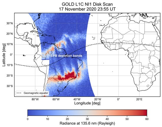
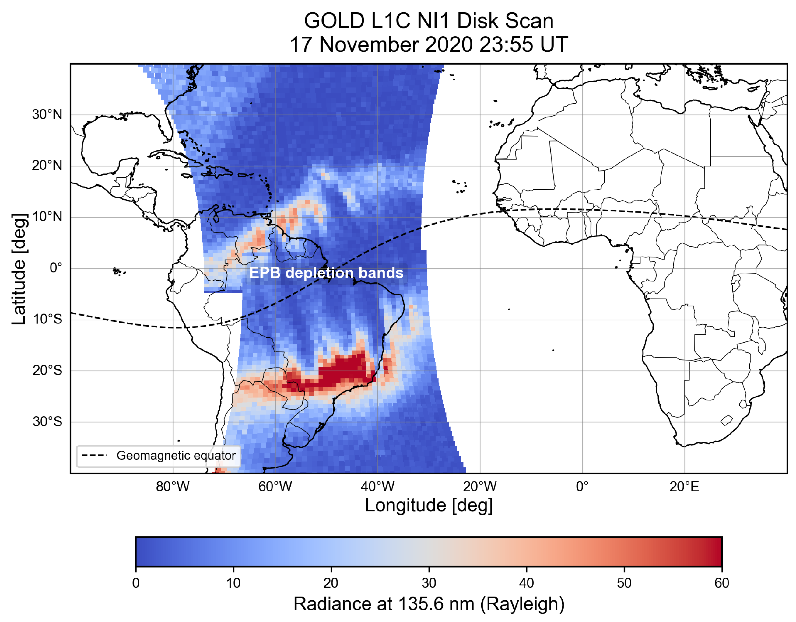
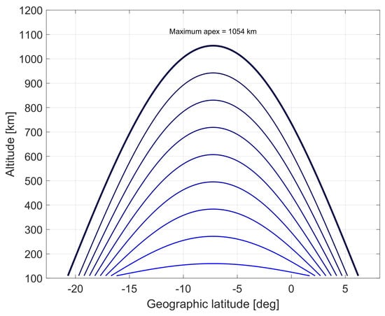
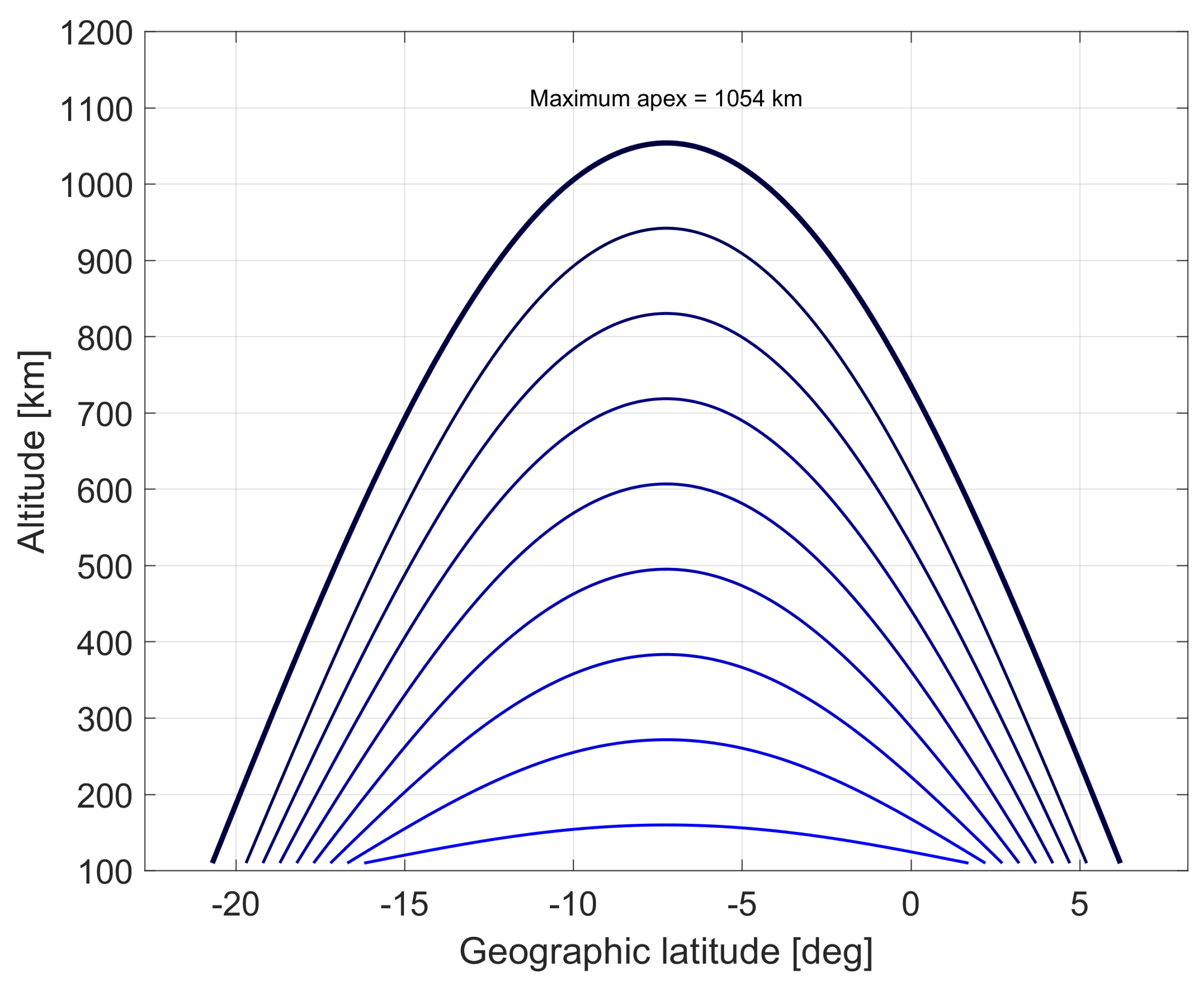
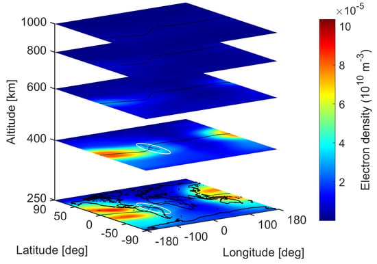
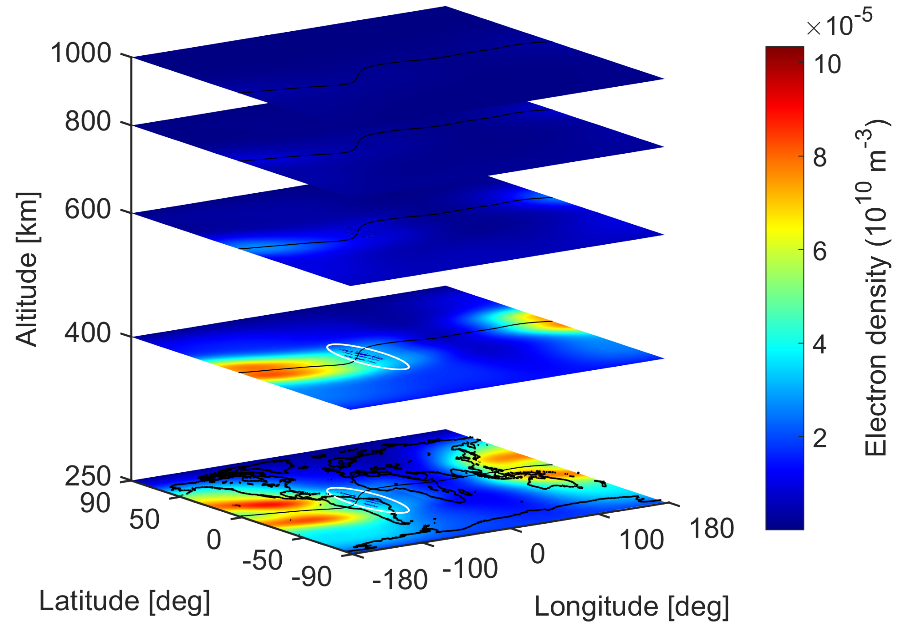
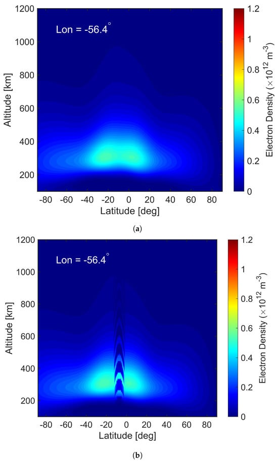
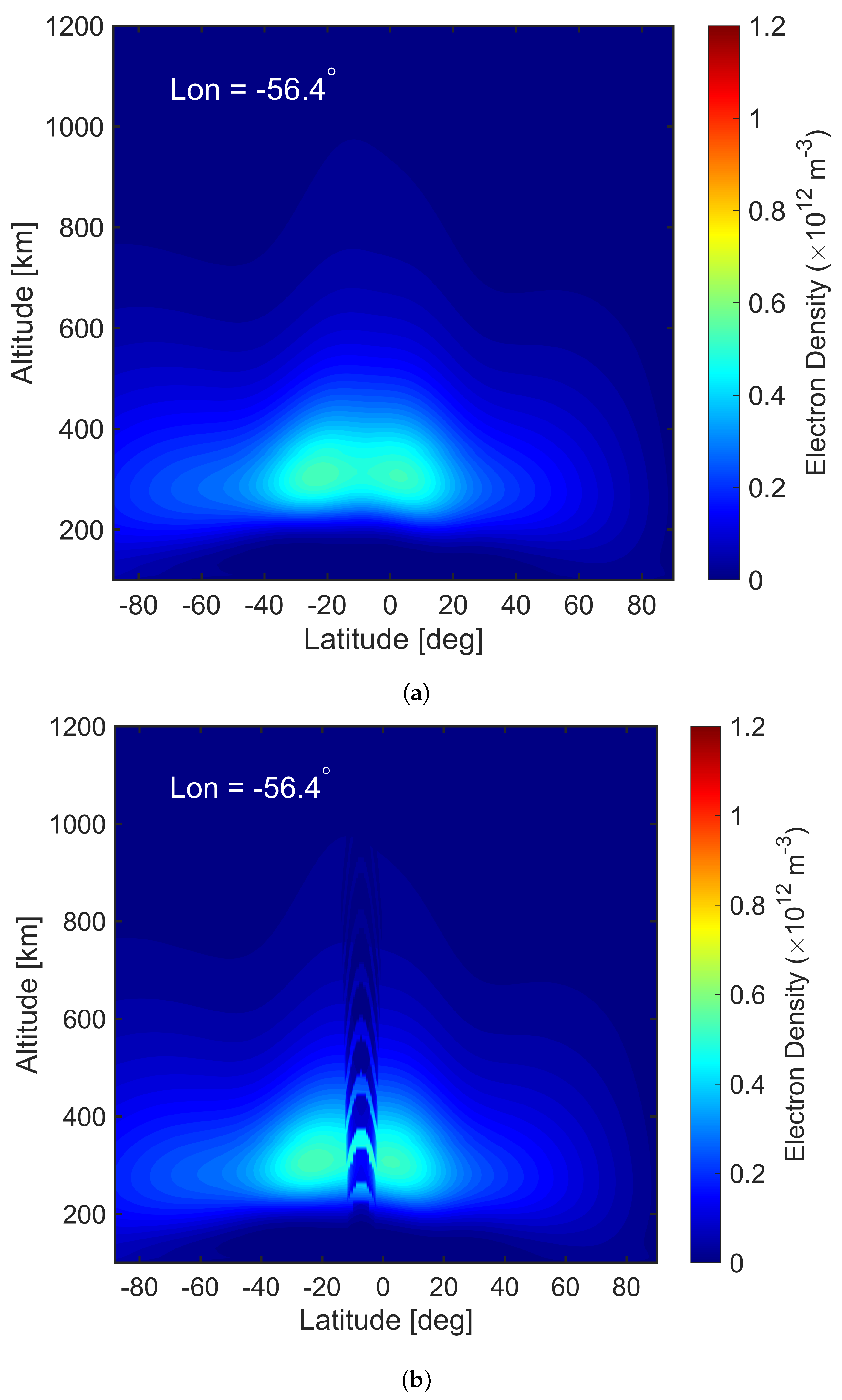
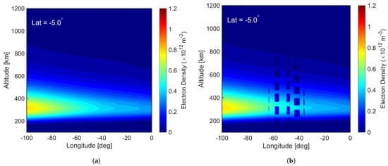
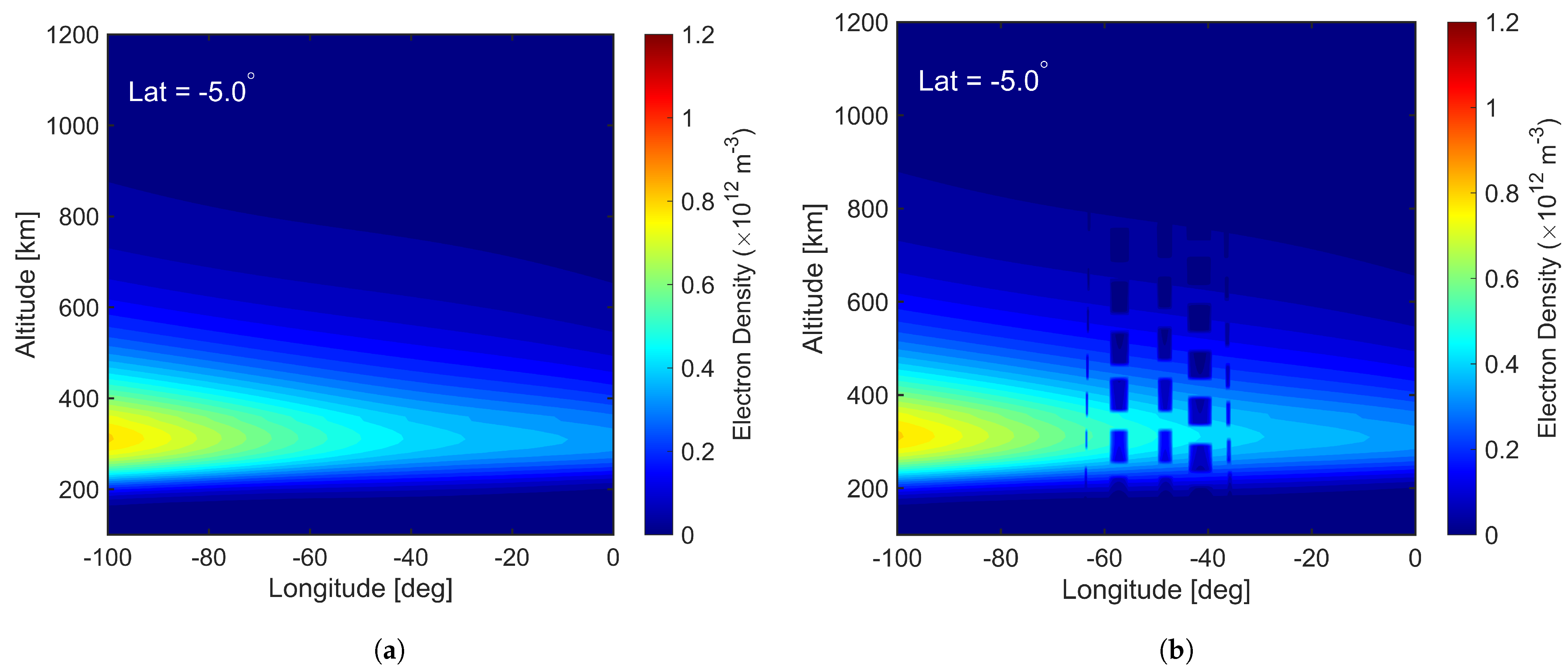
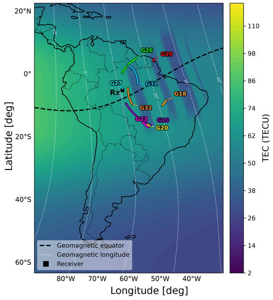
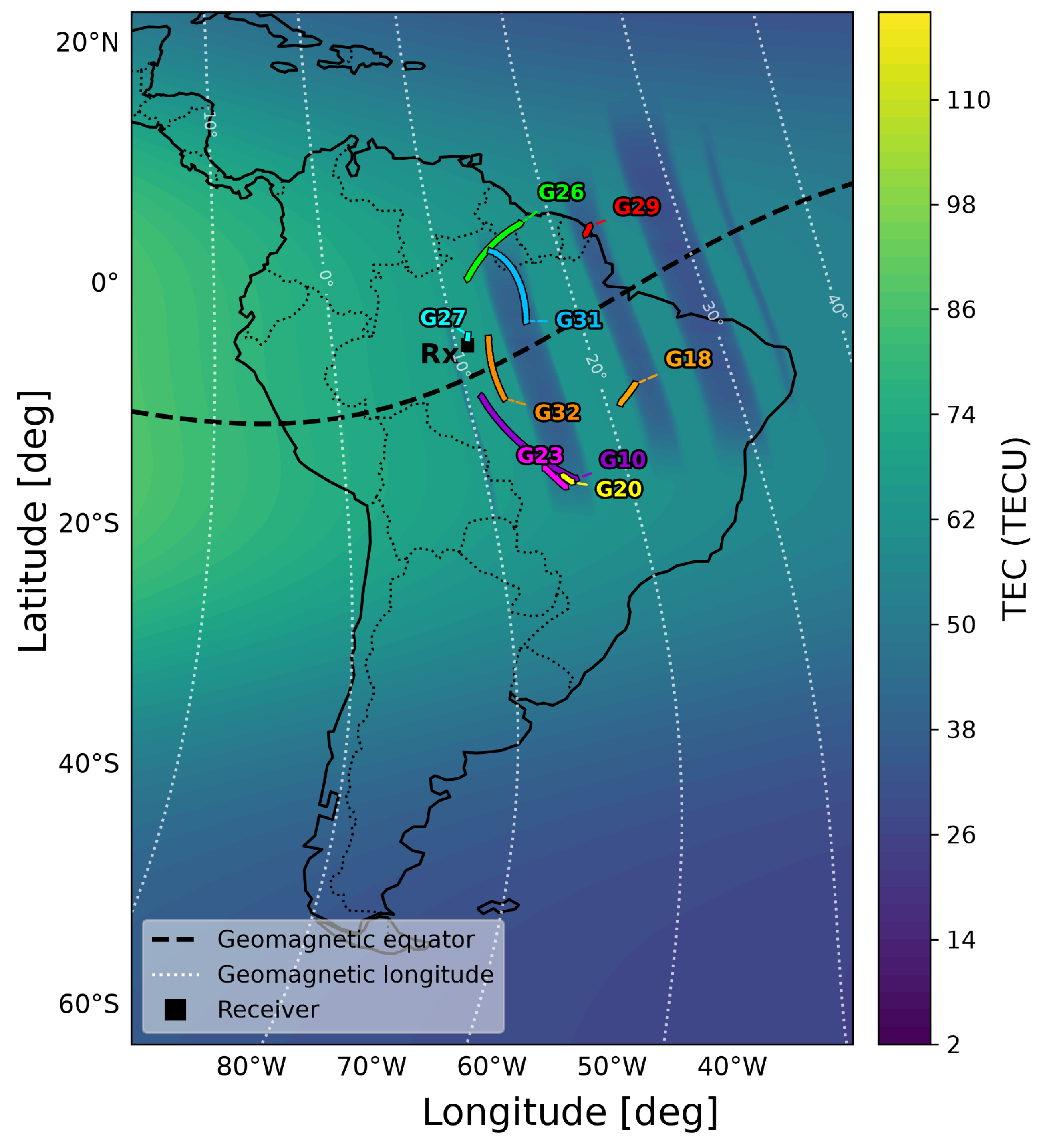
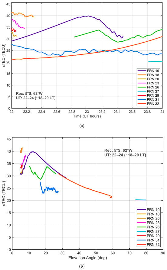
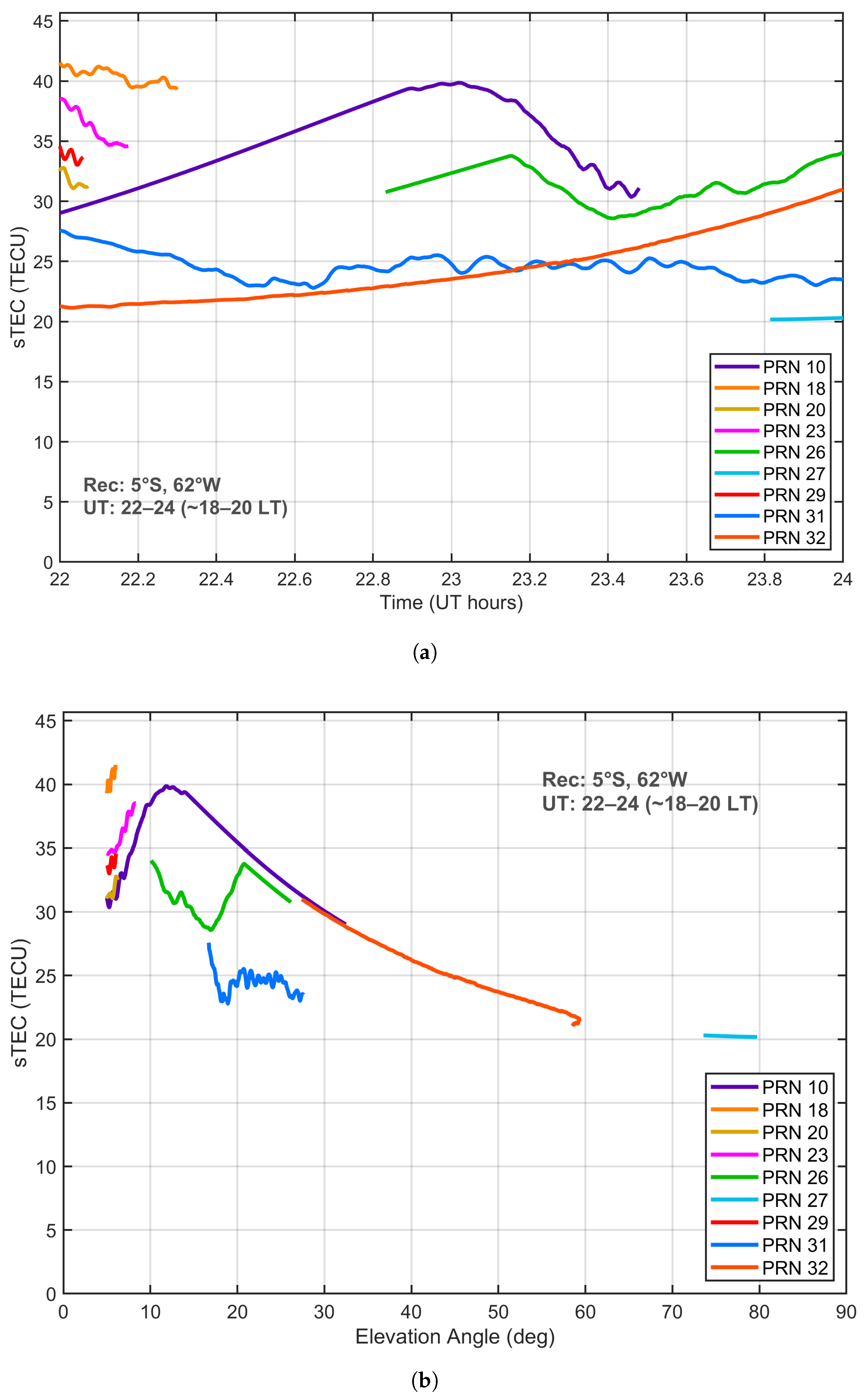
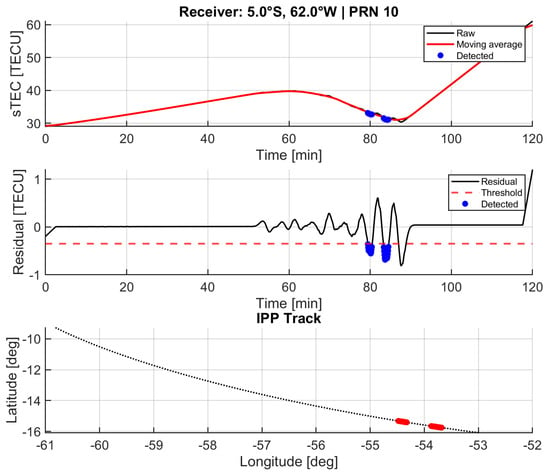
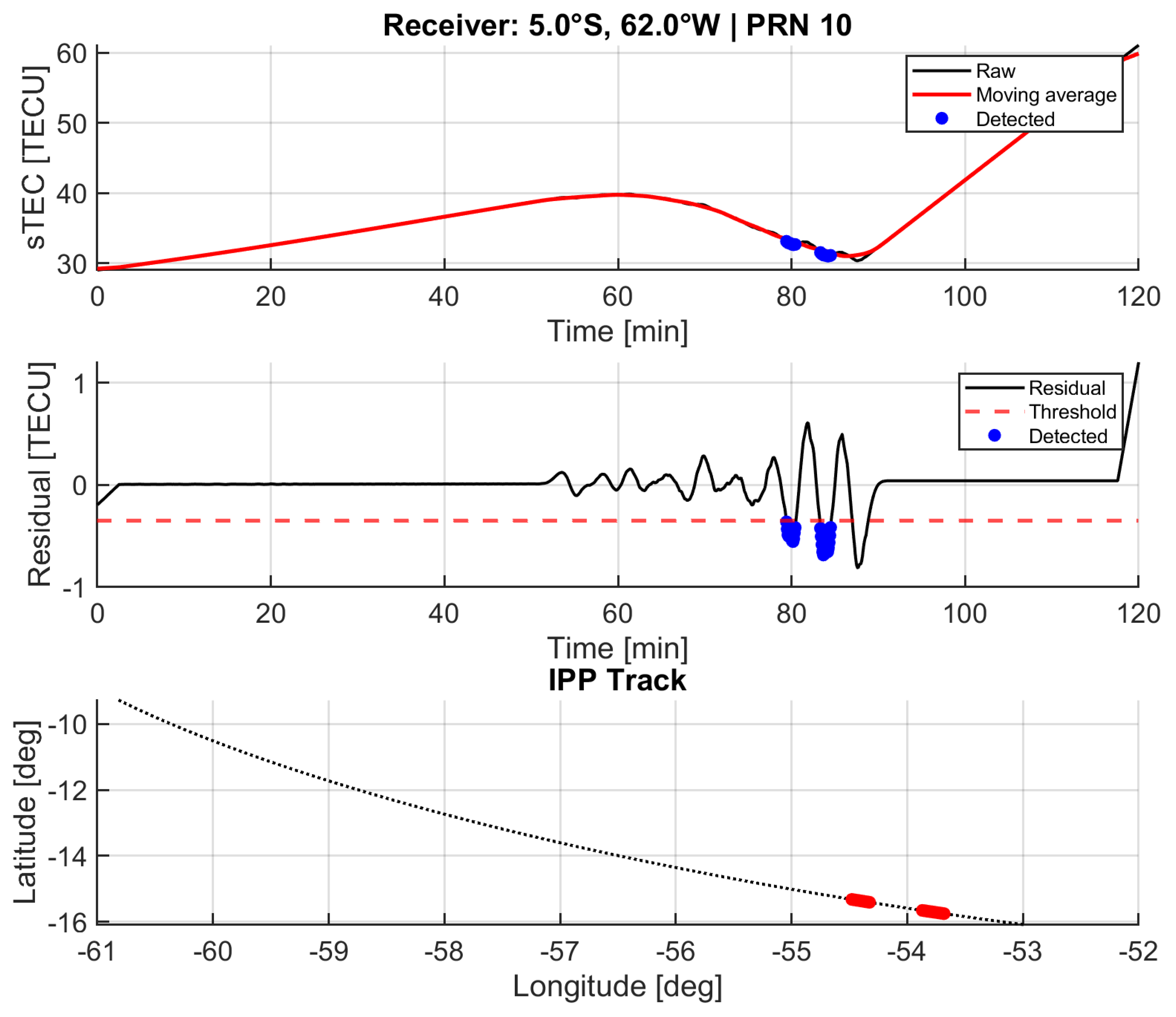
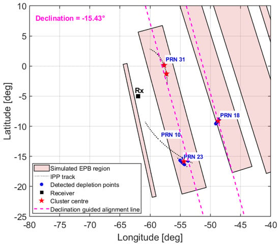
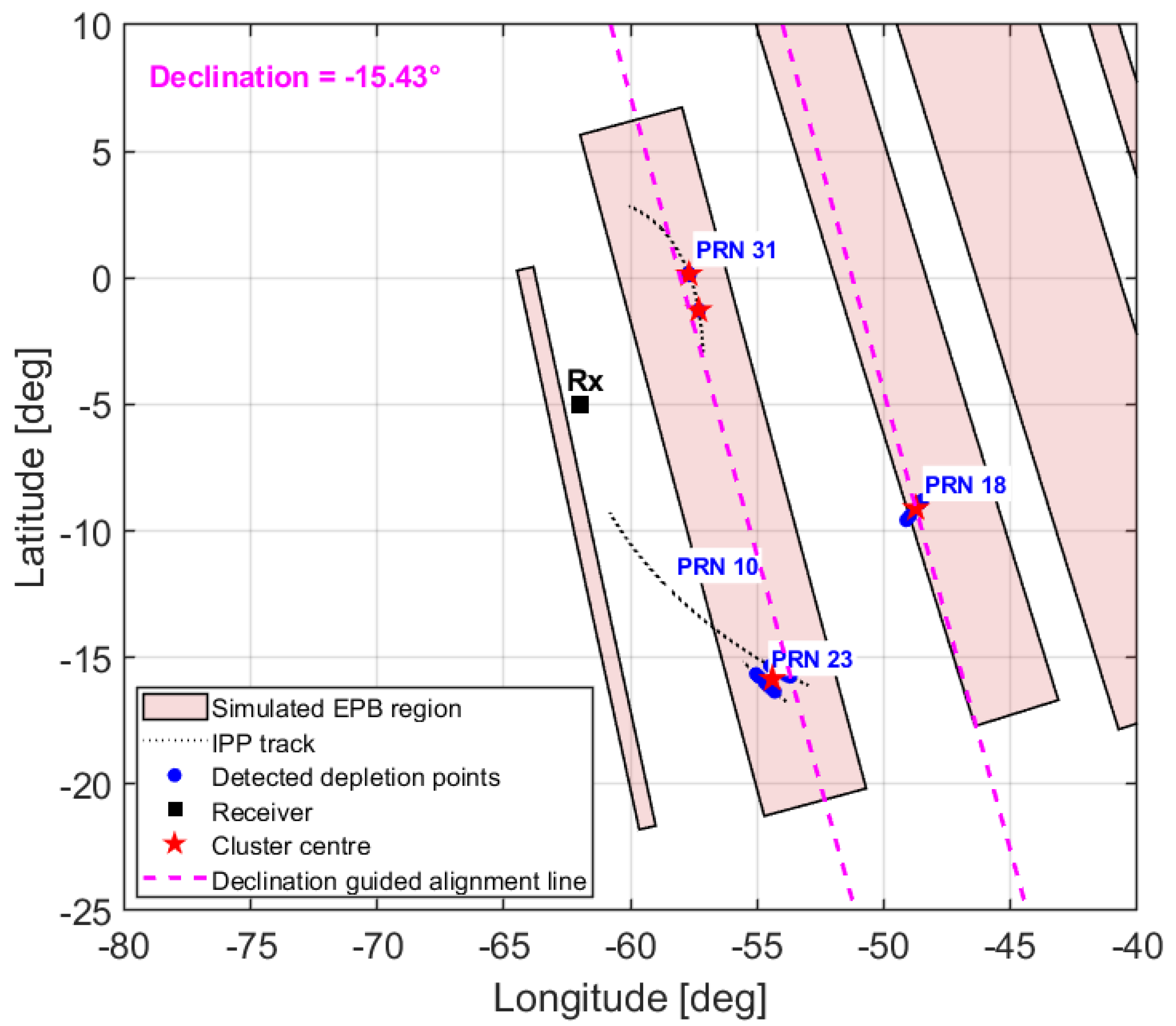
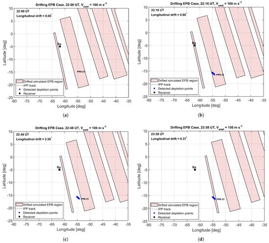
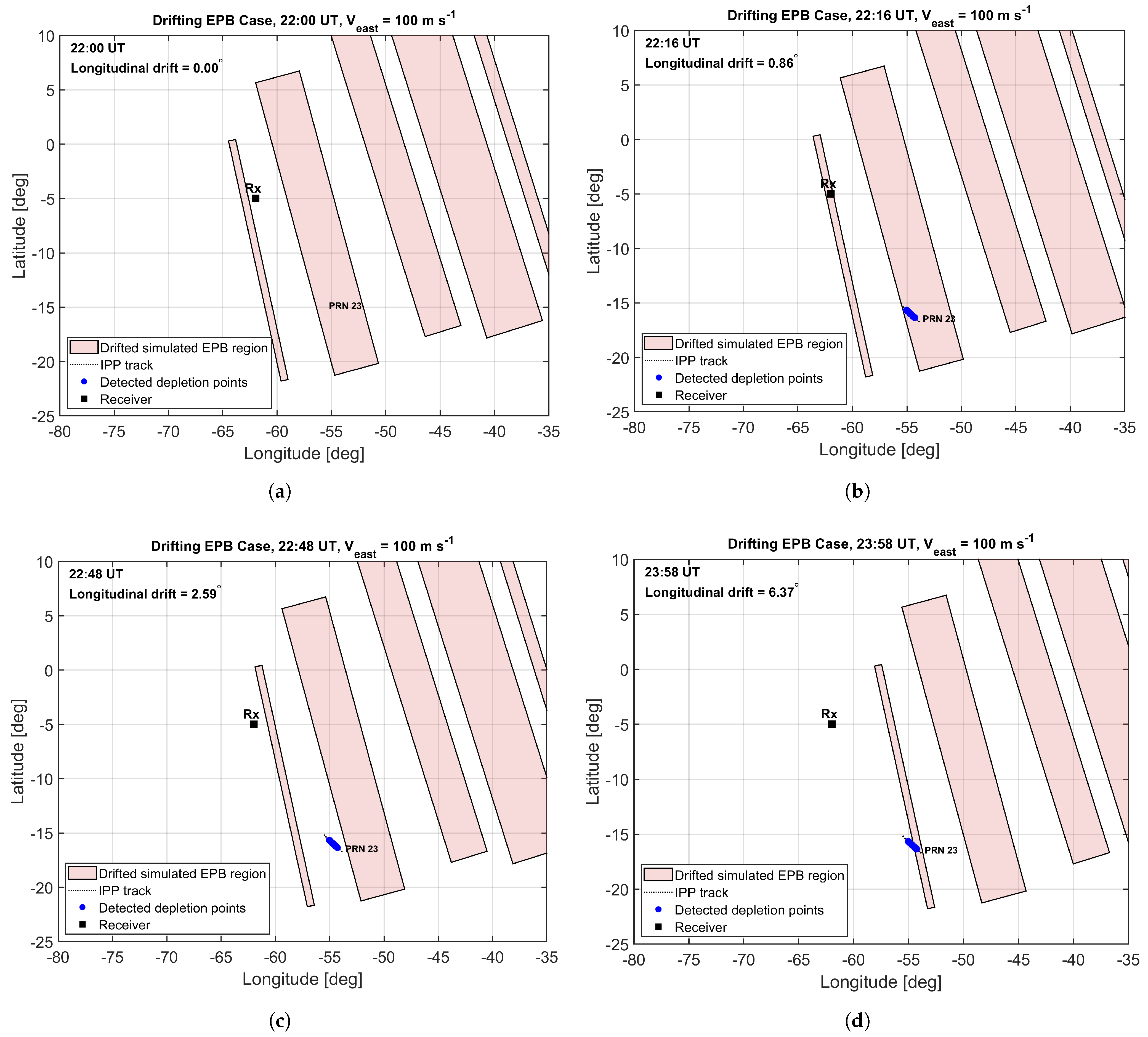
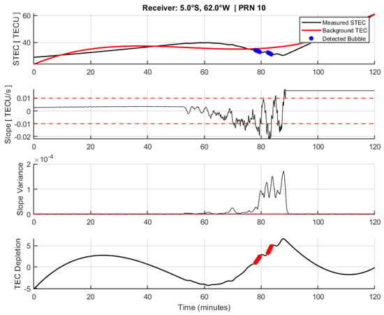
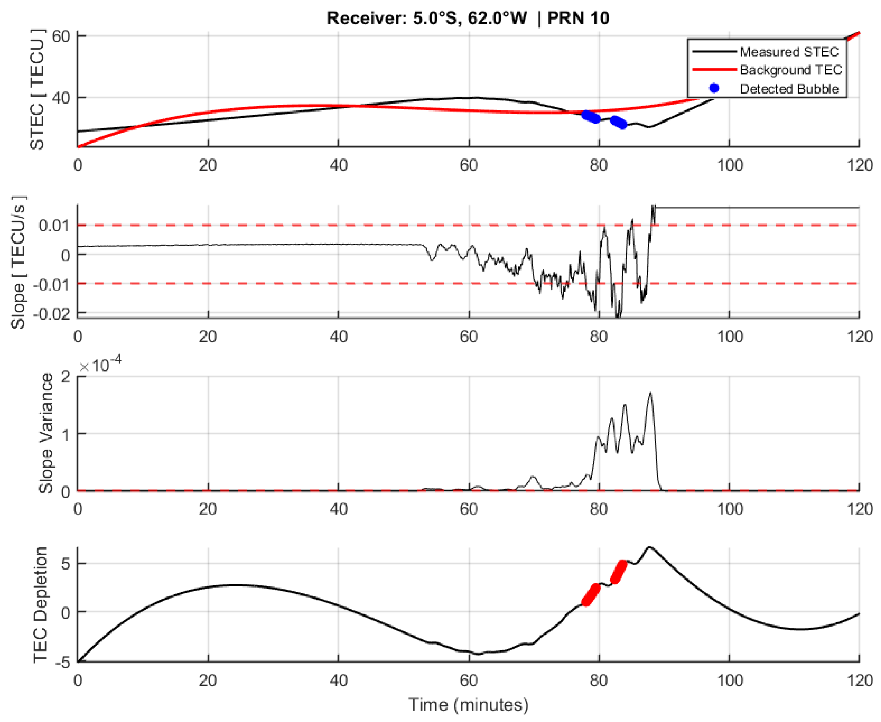
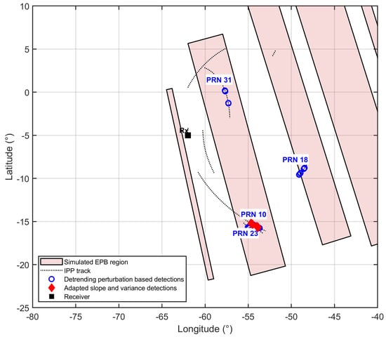
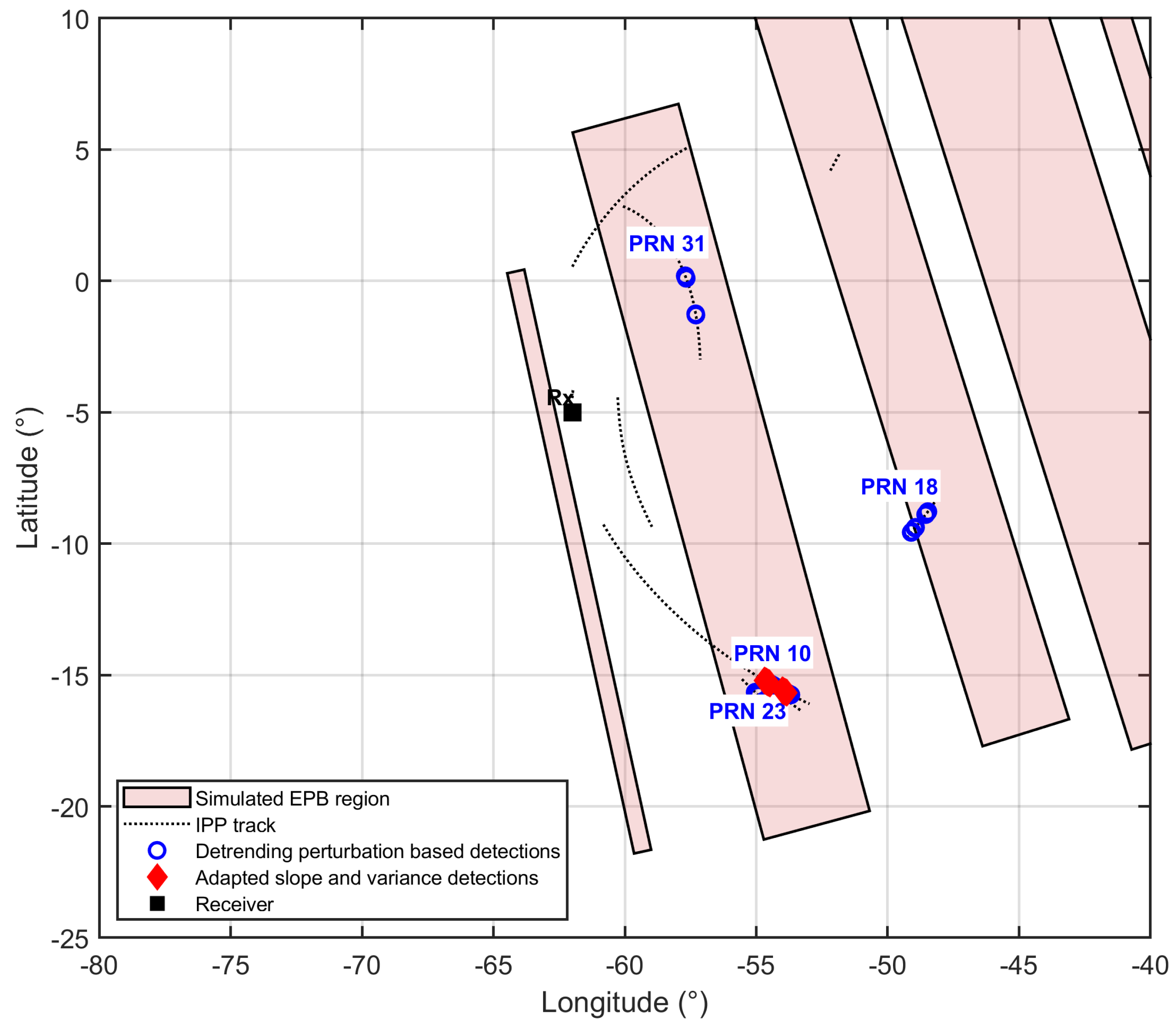

Disclaimer/Publisher’s Note: The statements, opinions and data contained in all publications are solely those of the individual author(s) and contributor(s) and not of MDPI and/or the editor(s). MDPI and/or the editor(s) disclaim responsibility for any injury to people or property resulting from any ideas, methods, instructions or products referred to in the content. |
© 2026 by the authors. Licensee MDPI, Basel, Switzerland. This article is an open access article distributed under the terms and conditions of the Creative Commons Attribution (CC BY) license.