3.1. RS Change Detection
The location and nature of change which has occurred in a watershed can be explicitly recognized using a post-classification comparison approach of land-cover change detection from RS images [
16]. This approach uses separate classifications of images acquired at different times to produce difference maps from which ‘‘from–to’’ change information can be generated [
17]. Among the several classifiers available, the Maximum Likelihood Classifier (MLC) has been widely used to classify RS data and successful results of applying this classifier for land-cover mapping have been numerous (e.g., [
18,
19,
20]) despite the limitations due to its assumption of normal distribution of class signatures [
21]. Its use has also been effective in a number of post-classification comparison change detection studies (e.g., [
12,
22,
23,
24]).While recent studies have indicated the superiority of newly developed image classification techniques based on Decision Trees (DT), Neural Networks (NN) and Support Vector Machines (SVM) over MLC (e.g., [
25,
26,
27,
28]), the advantage of MLC over these classifiers is significant owing to its simplicity and lesser computing time. This is crucial, especially for rapid land-cover mapping and change detection analysis of numerous multi-temporal images in a situation where time and computing resources are sorely limited. Moreover, the accuracy of any classifier is affected by the number of training samples and by selecting which bands to use during the classification. As reported by Huang
et al. [
25], improved classification accuracies of MLC, DT, NN and SVM can be achieved when training data size is increased and when more bands are included. In the case of Landsat image classification, improvements due to the inclusion of all bands exceeded those due to the use of a better classifier or increased training data size, underlining the need to use as much information as possible in deriving land-cover classification from RS images [
25]. All these aspects were considered in the detection and analysis of land-cover change in the Landsat images of the study area.
3.2. Landsat Image Pre-Processing
Orthorectified Landsat MSS and ETM+ images covering the study area acquired on 17 April 1976 (path 120, row 54) and 22 May 2001 (path 112, row 54), with pixel resolutions of 57-m and 28.5-m, respectively, were obtained from the Global Land-cover Facility (GLCF), University of Maryland (
http://glcf.umiacs.umd.edu). These images are part of the GLCF GeoCover collection which consists of decadal Landsat data which has been orthorectified and processed to a higher quality standard. Documentations on the orthorectification process can be found in the GLCF GeoCover website at
http://glcf.umiacs.umd.edu/research/portal/geocover/. All four bands of the 1976 Landsat MSS image and the seven bands of the 2001 Landsat ETM+ image were downloaded from the GLCF website.
Prior to any image pre and post processing, the geometric accuracy of the images were first assessed. For the Landsat ETM+ image, a total of thirty eight (38) points identifiable on both the image and 1:50,000 topographic maps of the same area published by the National Mapping and Resource Information Authority (NAMRIA) were used for the geometric accuracy assessment. These points were mostly road intersections and bridges. The Universal Transverse Mercator Zone 51 World Geodetic System 1984 (UTM 51 WGS84) grid coordinates of each point were determined both on the image and on the maps. Comparison of grid coordinates of these points in the 2001 Landsat image with those in the NAMRIA maps showed that the geometric accuracy of the image is acceptable with a global Root Mean Square Error (RMSE) of 10.25 meters and average local RMSE of 10.05, which are both less than half a pixel (<14.25 m).
The co-registration of the 1976 Landsat image to the 2001 Landsat image was next performed. In this case, the 2001 Landsat image is the reference image where the UTM coordinates of points on the 1976 Landsat image were compared. Based on 22 points common in both images, the global RMSE was computed as 16.62 m, with average local RMSE of 15.20 m. This indicates that the geometric accuracy of the 1976 Landsat image is acceptable and its co-registration with the 2001 Landsat image is good. Furthermore, as the global RMSE and average local RMSE is less than half a pixel (or 28.5 m), the 28.5-m resolution land-cover map derived from the 2001 Landsat image after undergoing resampling to 57-m resolution, will correctly align with the land-cover map derived from this 1976 Landsat image. This minimizes the error due to image misregistration in the change detection and analysis.
The Landsat images were then radiometrically corrected to at-sensor radiance using the standard Landsat image calibration formulas and constants [
29,
30]. A fast atmospheric correction using dark-object subtraction using band minimum [
31] was also implemented. Normalized Difference Vegetation Index (NDVI) images were also computed from the radiometrically and atmospherically-corrected radiance images and used as an additional band during image classification. Only the portions of the images covering the study area were subjected to image analysis. All image processing was done using Environment for Visualizing Images (ENVI) Version 4.3 software.
2.3. Image Classification and Land-Cover Change Detection
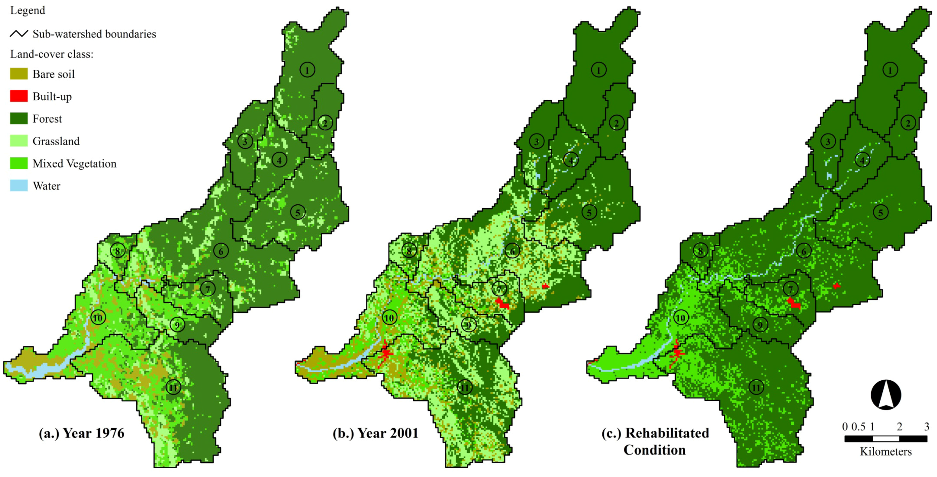
Six (6) land-cover classes were identified from the images through visual interpretations with the aid of ancillary datasets such as 1:50,000 NAMRIA topographic maps with map information obtained in 1977 (through aerial photography campaigns), Google Earth Images, and 1:250,000 2003 DENR land-cover and forest cover maps. This study acknowledges the limitation introduced by the absence of ground truth land-cover data necessary for the interpretation of the 1976 Landsat MSS image. Hence, the use of old topographic maps was imperative as a source of information for interpreting major land-cover classes in the 1976 Landsat image.
The land-cover classes include barren areas, built-up areas, forest, grassland, mixed vegetation (combination of forest, tree plantation, shrub land and grassland) and water bodies. In this study, each land-cover class is identified as closely as possible to the definitions by Anderson
et al. [
32]. Barren areas are defined as those portions of the watershed with exposed soil and in which less than half of an areal unit has vegetation or other cover while built-up areas are those portions of intensive human use with much of the land covered by structures. The forest class is defined as a parcel of land having a tree-crown areal density of 10% or more, and is stacked with trees capable of producing timber or other wood products. Grasslands are those portions where the natural vegetation is predominantly grasses and/or grass-like plants.
Built-up areas within the study area were only detected on the 2001 Landsat ETM+ image. We assumed that built-up areas in the 1976, although present, were limited in extent and sparsely distributed so that they were not visible in the Landsat MSS images primarily because of the sensor’s low spatial resolution. Representative samples of each class were collected from the images for supervised image classification (
Table 1). The training set comprised, as a minimum, a sample of typically 10–30 pixels per class per band [
33], and were collected in such a way that the assumption of normal distribution of the MLC is satisfied and can provide an appropriate summary of the data’s distribution from which a representative estimate of the mean and variance may be derived [
28]. It was also ensured that the separability of the classes, computed using the Jeffries-Matusita Distance [
34], is ≥1.7. Another independent set of samples were likewise collected for accuracy assessment. A minimum number of 30 ground truth pixels were randomly chosen for each class, following the guidelines of Van Genderen
et al. [
35] to obtain a reliable estimate of classification accuracy of at least 90%.
Table 1.
Land-cover classes identified from the Landsat MSS and ETM+ images of the study area with number of samples collected for classifier training and accuracy assessment.
Table 1.
Land-cover classes identified from the Landsat MSS and ETM+ images of the study area with number of samples collected for classifier training and accuracy assessment.
| Land-Cover Class | Number of Pixels for Classifier Training | Number of Pixels for Accuracy Assessment |
|---|
| 1976 Landsat MSS | 2001 Landsat ETM+ | 1976 Landsat MSS | 2001 Landsat ETM+ |
|---|
| Barren Areas | 182 | 170 | 40 | 54 |
| Built-up Areas | - | 52 | - | 30 |
| Forest | 222 | 371 | 64 | 96 |
| Grassland | 122 | 220 | 62 | 91 |
| Mixed Vegetation | 139 | 149 | 58 | 54 |
Water
(along rivers and streams) | 168 | 92 | 30 | 48 |
The MLC was used to classify the two Landsat images. For the 1976 Landsat image classification, all the four bands and the derived NDVI image were subjected to classification. The same was done for the classification of the 2001 Landsat ETM+ image where all the seven bands and the NDVI were utilized.
The accuracies of each classified image were independently assessed. Four measures were used to assess the accuracy of the classified images namely, the overall classification accuracy, kappa statistic, producer’s accuracy (PA) and user’s accuracy (UA) [
36]. Initial trials were done to classify the input images using the Minimum Distance, Mahalanobis Distance and Parallepiped classifiers. However, the accuracies of each classified image using these classifiers were significantly lower (<90%) than those of the MLC-classified images. The two resulting land-cover maps were then subjected to post-classification comparison change detection analysis to examine the location, extent and distribution of land-cover change in the study area. The 2001 land-cover map was first re-sampled to 57-m resolution using nearest neighbor method prior to change detection.
3.2. Hydrologic Modeling
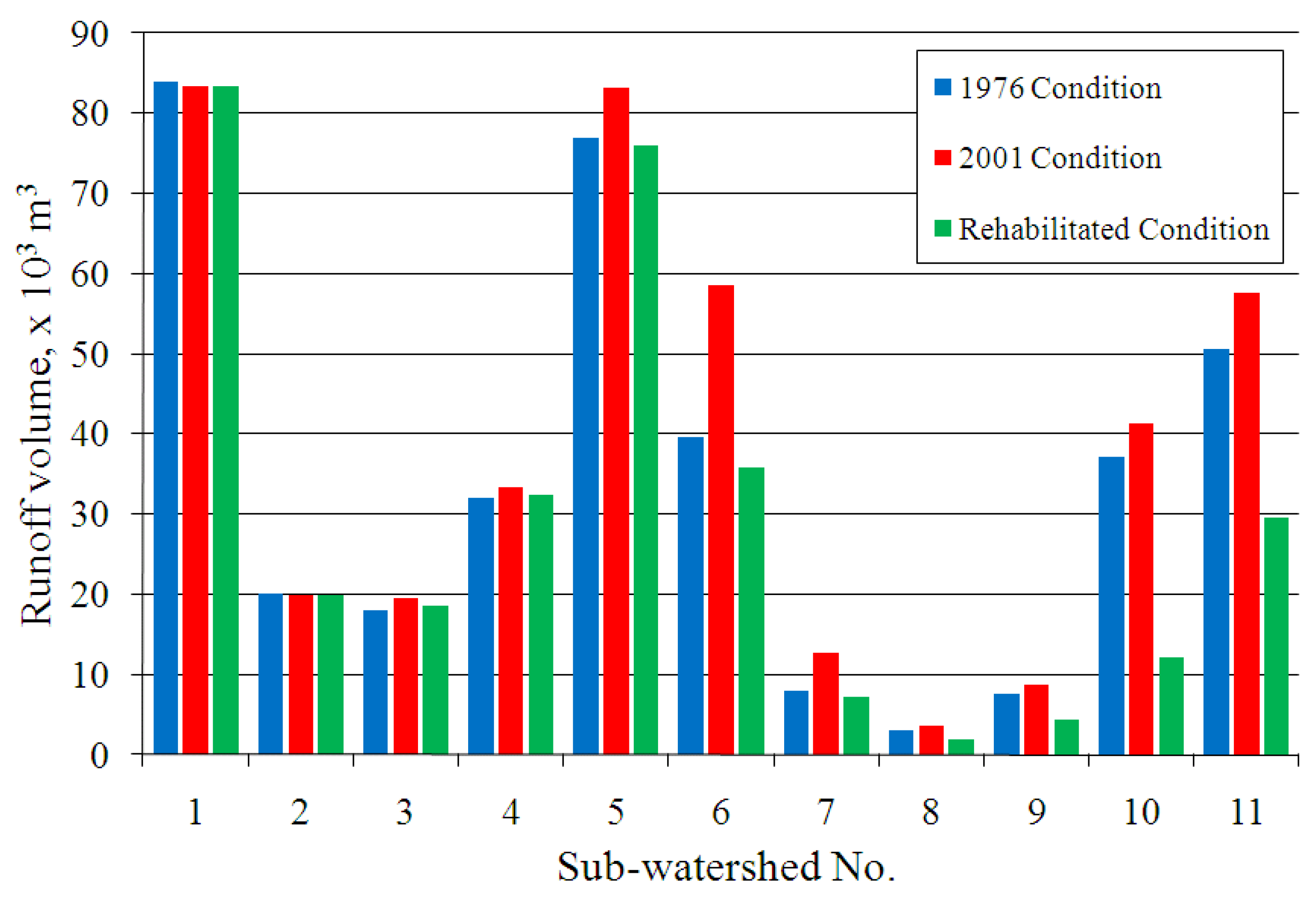
The land-cover information derived from the analysis of the Landsat images were integrated into a hydrologic model as a means of estimating the impacts of the differences in land-cover conditions to the hydrological processes of the watershed, specifically in the generation of runoff during rainfall events.
Hydrologic modeling was performed using the Soil Conservation Service-Curve Number (SCS-CN) model [
15]. The SCS-CN model, also called the runoff curve number method, for the estimation of direct runoff from storm rainfall is a well established method in hydrologic engineering and environmental impact analyses and has been very popular because of its convenience, simplicity, authoritative origins, and its responsiveness to four readily grasped watershed properties: soil type, land-use/land-cover and treatment, surface condition, and antecedent moisture condition [
37]. The popular form of the SCS-CN model is:
where
P is total rainfall,
Ia is initial abstraction,
Q is direct runoff,
S is potential maximum retention which can range (0, ∞), and
λ is initial abstraction coefficient or ratio. All variables are in millimeters (mm) except for
λ which is unitless. The initial abstraction
Ia includes short-term losses due to evaporation, interception, surface detention, and infiltration and its ratio to
S describes
λ which depends on climatic conditions and can range (0, ∞). The SCS has adopted a standard value of 0.2 for the initial abstraction ratio [
15] but this can be estimated through calibration with field measured hydrologic data. The potential maximum retention
S characterizes the watershed’s potential for abstracting and retaining storm moisture, and therefore, its direct runoff potential [
37].
S is directly related to land-cover and soil infiltration through the parameter
CN or “curve number”, a non-dimensional quantity varying in the range (0–100) and depends on the antecedent moisture condition of the watershed. Higher
CN values indicate high runoff potential. For normal antecedent moisture conditions (AMCII, 5-day antecedent rainfall (AR) is 12.7–27.94 mm), the
CN values for land-cover types and soil textures (hydrologic soil groups B and D) prevalent in the study area are shown in
Table 2. Spatially distributed soil texture data converted into a hydrologic soil group (HSG) map was obtained from the 1:150,000 soil map of the Philippines published by the Philippines’ Bureau of Soils and Water Management of the Department of Agriculture.
The AMCII CN values can be converted to AMCI (dry condition, AR < 12.7 mm) and AMCIII (wet condition, AR > 27.94 mm) using the formulas of Chow
et al. [
38] as
where
CN(I),
CN(II) and
CN(III) are the
CN values under AMC I, II and III, respectively.
The SCS-CN model was implemented using the Hydrologic Engineering Center-Hydrological Modeling System or HEC-HMS Version 3.3 [
39]. The SCS-CN model was co-implemented with the Clark Unit Hydrograph method (for sub-watershed routing of runoff), the Exponential Baseflow Recession model, and the Muskingum-Cunge model for channel routing. A thorough discussion of these three additional models can be found in Chow
et al. [
38]. Model parameterizations were done using HEC-GeoHMS [
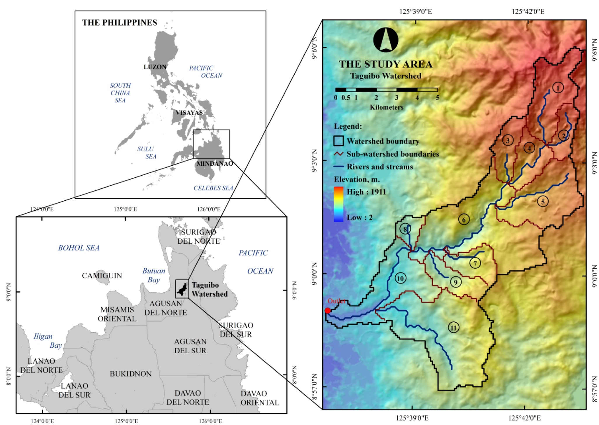
40], the ArcView GIS-based pre-processor of HEC-HMS. HEC-GeoHMS was used to delineate 11 sub-watershed boundaries and reproduce topologically-correct stream networks through a series of steps collectively known as terrain pre-processing, by utilizing the surface topography information from a 90 m spatial resolution Shuttle Radar Topography Mission Digital Elevation Model (SRTM DEM) as the origin of the boundaries and stream network.
Average CN values for each sub-watershed were computed based on the 2001 and 1976 land-cover maps. Sub-watershed time of concentration and storage coefficient parameters of the Clark Unit Hydrograph model as well as initial values of the baseflow recession constant in each sub-watershed were first assumed but these values were later optimized during the calibration stage. Muskingum-Cunge model parameter values were obtained from profile and cross-section surveys of the major streams conducted on April 2007.
Table 2.
AMCII CN values for different land-cover types under hydrologic soil groups B and D which are prevalent in the study area. (Source: SCS National Engineering Handbook [
15]).
Table 2.
AMCII CN values for different land-cover types under hydrologic soil groups B and D which are prevalent in the study area. (Source: SCS National Engineering Handbook [15]).
| Land-Cover | AMCII Curve Number (CN) |
|---|
| Soil Group B | Soil Group D |
|---|
| Barren areas | 86 | 94 |
| Built-up areas | 74 | 86 |
| Forest | 55 | 77 |
| Grassland | 61 | 80 |
| Mixed Vegetation | 58 | 79 |
| Water | 98 | 98 |
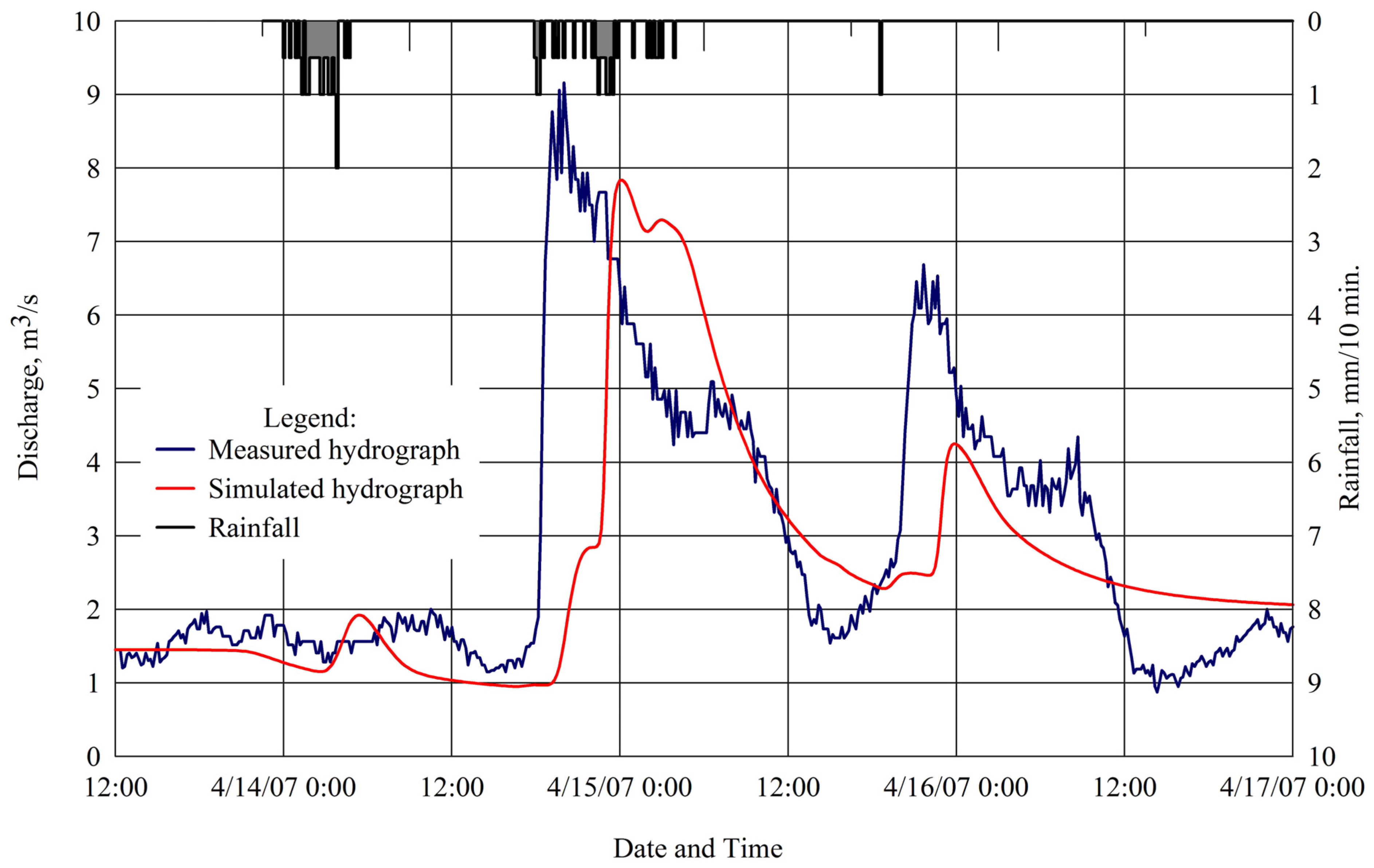
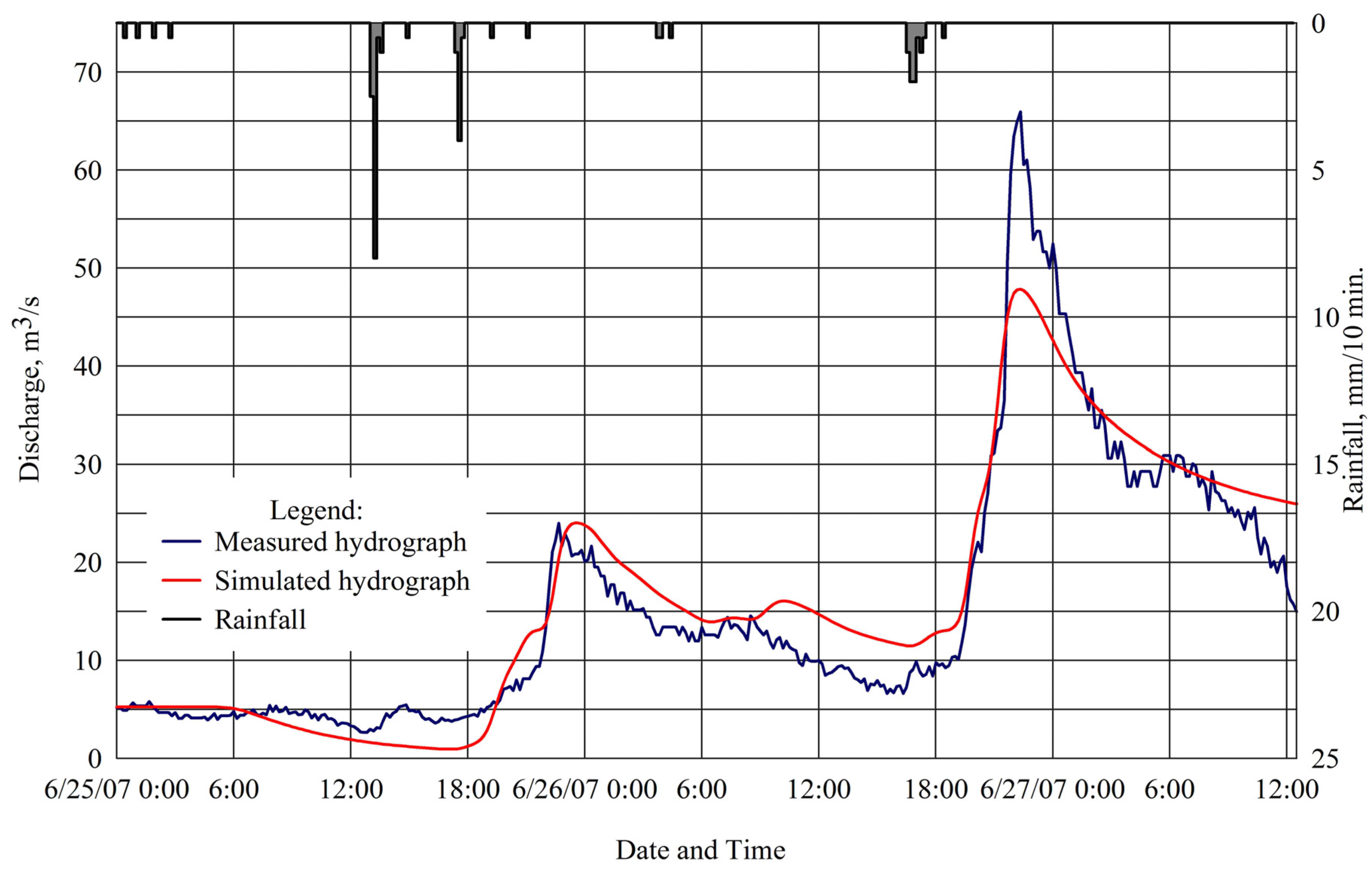
The HEC-HMS model was calibrated using rainfall events recorded at the middle portion of the watershed, and 10-minute discharge hydrographs measured at the main outlet for the 25–27 June 2007 period. Records of 5-day accumulated rainfall depths before the simulation showed an AR > 27.94 mm, indicating AMCIII. Hence, the AMCII
CN values were transformed to AMCIII
CN using Chow
et al.’s formula [
38]. The absence of sources of land-cover information for the state of the watershed when the calibration data were collected prompted us to parameterize the model using the 2001 land-cover map. During this period, available satellite images were all covered with a significant amount of cloud (>20% of scene) that totally hindered the derivation of accurate and complete land-cover information.
The hydrologic model calibration made use of the available automatic calibration utility in HEC-HMS. This procedure was done to simultaneously fine-tune the λ parameter of the SCS-CN model, and the time-related parameters of the Exponential Baseflow Recession model and Clark Unit Hydrograph model, which were initially assumed. This step includes adjustments or optimizations of the initial values of these parameters until the overall model results acceptably match the measured discharge data.
HEC HMS uses the peak-weighted root mean square error (PWRMSE) as the objective function to minimize during calibration. Parameters of the model were adjusted iteratively until the PWRMSE is minimized. PWRMSE is implicitly a measure of the comparison of the magnitudes of the peaks, volumes, and times of peak of the simulated and measured hydrographs. The Nelder and Mead (NM) algorithm [
41] was used to minimize the PWRSME by identifying the most reasonable parameter values that will yield the best fit of computed to the observed hydrograph.
The model was then validated with 10-minute discharge data measured on 13–17 April 2007 where the watershed is in AMC II. Only the CN, Ia, baseflow recession constant and time-related parameters of the hydrologic model were changed to reflect the actual condition of the watershed during this period.
The Nash-Sutcliffe Coefficient of Model Efficiency,
E [
42], was used to evaluate the performance of the hydrologic model after calibration and during the validation process.
E is a normalized, dimensionless statistic that determines the relative magnitude of the residual variance (“noise”) compared to the measured data variance and indicates how well the plot of observed
versus simulated data fits the 1:1 line.
E ranges between −∞ and 1.0 (1 included) with
E = 1 being the optimal value. Values between 0.0 and 1.0 are generally viewed as accepted levels of performance while values ≤ 0.0 indicates that the mean observed value is a better predictor than the simulated value, which indicates unacceptable model performance [
43].


