Radiometric Normalization of Temporal Images Combining Automatic Detection of Pseudo-Invariant Features from the Distance and Similarity Spectral Measures, Density Scatterplot Analysis, and Robust Regression

Abstract

Radiometric precision is difficult to maintain in orbital images due to several factors (atmospheric conditions, Earth-sun distance, detector calibration, illumination, and viewing angles). These unwanted effects must be removed for radiometric consistency among temporal images, leaving only land-leaving radiances, for optimum change detection. A variety of relative radiometric correction techniques were developed for the correction or rectification of images, of the same area, through use of reference targets whose reflectance do not change significantly with time, i.e., pseudo-invariant features (PIFs). This paper proposes a new technique for radiometric normalization, which uses three sequential methods for an accurate PIFs selection: spectral measures of temporal data (spectral distance and similarity), density scatter plot analysis (ridge method), and robust regression. The spectral measures used are the spectral angle (Spectral Angle Mapper, SAM), spectral correlation (Spectral Correlation Mapper, SCM), and Euclidean distance. The spectral measures between the spectra at times t1 and t2 and are calculated for each pixel. After classification using threshold values, it is possible to define points with the same spectral behavior, including PIFs. The distance and similarity measures are complementary and can be calculated together. The ridge method uses a density plot generated from images acquired on different dates for the selection of PIFs. In a density plot, the invariant pixels, together, form a high-density ridge, while variant pixels (clouds and land cover changes) are spread, having low density, facilitating its exclusion. Finally, the selected PIFs are subjected to a robust regression (M-estimate) between pairs of temporal bands for the detection and elimination of outliers, and to obtain the optimal linear equation for a given set of target points. The robust regression is insensitive to outliers, i.e., observation that appears to deviate strongly from the rest of the data in which it occurs, and as in our case, change areas. New sequential methods enable one to select by different attributes, a number of invariant targets over the brightness range of the images.

1. Introduction

Spectral images acquired from the same area at different times contain valuable information for regular monitoring of the Earth’s surface, allowing us to describe the land-cover evolution, vegetation phenology, and natural hazard events. However, it is difficult to maintain radiometric accuracy in orbital images due to changes in atmospheric conditions, Earth-Sun distance, detector calibration, illumination angles, viewing angles, and sensor oscillation, as are required in order to highlight the spectral changes of interest. Another common problem in change-detection analysis from different sensors, such as Landsat Thematic Mapper (TM) and Landsat Enhanced Thematic Mapper plus (ETM+) images is that they, additionally, require the evaluation of radiometric consistency between sensors to ensure comparability between the temporal images [1,2]. Thus, methods for ensuring radiometric consistency among temporal images are necessary to remove, or compensate for, all the above effects, except for actual changes on the land surface, allowing the surface reflectance or normalized digital numbers obtained under different conditions to be placed on a common scale [3].

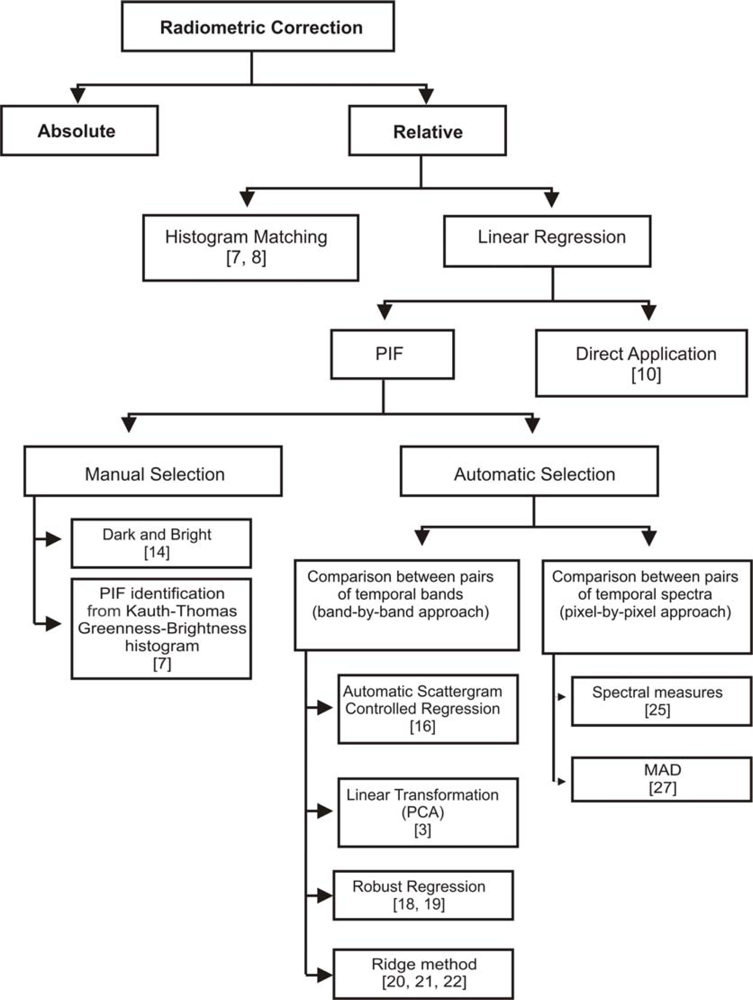
In previous studies, two levels of radiometric correction were developed: absolute and relative [1,4–6] (Figure 1). In absolute radiometric correction, atmospheric radiative-transfer codes are used to obtain the reflectance at the Earth’s surface from the measured spectral radiances. The absolute method corrects for following factors: changes in satellite sensor calibration over time, differences among in-band solar spectral irradiance, solar angle, variability in Earth-Sun distance, and atmospheric interferences. In contrast, relative correction by normalization does not find the true radiance of the surface or remove atmospheric errors, but instead transforms the digital numbers to a common scale [3]. Thus, the radiometric properties of an image are adjusted to match a reference image [7,8], image normalization uses a histogram-matching method [9] or a linear-regression method [10].

The linear regression method is the most widely used approach for relative correction. Initially, the technique was based on simple regression that considered all the pixels of temporal images [10]. Subsequently, normalization was performed considering landscape elements with reflectance values that are nearly constant over time, ‘pseudo-invariant features’, or PIFs [7,11–13]. Therefore, the key problem of the image regression is to obtain an appropriate procedure for a selection of PIFs. For the regression model to be reliable, selection of radiometric control targets must consider the following characteristics [11,14,15]: small changes in elevation for which the thickness of the atmosphere over each target is approximately the same; minimal amounts of vegetation due to high susceptibility changes over time; positioning in flat areas in order to minimize the influence of changes in sun angle between the images; and a large range of brightness values. PIF selection can be made by visual inspection or through computational methods.

PIF selection through visual inspection establishes regions of interest for the dark and bright (DB) areas [14]. In this objective, the PIFs can be selected using scatterplots with Kauth-Thomas (KT) greenness-brightness components [7]. However, visual inspection methods are subjective and dependent on the analyst’s selection, which can decrease accuracy.

Computational methods for PIF selection are more accurate, considering an automatic extraction. There are two main strategies, which consider the different dimensions of the image (X, Y, and Z components): (a) band-by-band methods that compare a pair of bands at different times (X and Y dimensions of the image), and (b) pixel-by-pixel methods that compare a pair of spectra at different times for a pixel (Z dimension of the image).

PIF detection methods that perform comparisons between pairs of bands are the most commonly used. These include no-change buffer zone around a fitted line from linear regression [16] or principal components [2,3,17]; robust-regression [18,19]; scatter-plot density [20–22]. Generally, two attributes are used to identify the PIFs: invariant point density and residual values obtained from differences between observed and estimated values from the linear model.

Elvidge et al.[16] proposed a method called automatic scattergram controlled regression (ASCR), which performs a linear regression between the temporal image pairs and calculates a no-change buffer zone from the orthogonal distances between the points and the fitted straight-line. Du et al.[3] selected the PIFs using principal component analysis (PCA) and a no-change buffer zone. The authors consider the most probable linear relationship between two individual bands is described by the first principal component. The pattern of pixel distribution resembles an ellipse, described adequately by the major and minor PC axes. The quality control of the method establishes a range around the primary major axis (no-change buffer zone), until obtaining an acceptable linear correlation coefficient (r) of candidate PIFs from the two images. This procedure limits the no-change buffer zone from the minor PC axes (orthogonal to the first axis) which shows the deviations to the main axis. In addition, the user can apply thresholds for rejecting cloudy and water pixels. Although the method improves the optimal linear regression model, it still has problems. If the invariant point density is too low the sample will not be well-represented in first component. Thus, there is a tradeoff between the sample size and the correlation coefficient. The main limitation of these two methods is the elimination of outliers in a single step (no-change buffer zone). If the initial data contain many outliers, the first estimate of the linear regression or PCs can be wrong, as the subsequent steps of buffer zone and the elimination of outliers. The reliability of the first straight-line is of high importance for the solution, however, this is not always possible. Furthermore, a marked reduction in the buffer zone can have a result similar to the first straight-line.

Limitation in the use of the buffer zone indicates the need for a different approach, already described in statistical science in the 1970s [23,24]. The theory of multidimensional robust estimators searches the identification of outliers by successive interactions. Robust-regression is a form of the regression analysis insensitive to outliers, i.e., observations, which do not follow the pattern of the other observations, and they have serious effects on statistical inference. Thus, this procedure is an improvement to least squares, which fit a model from the valid observations. Heo and FitzHugh [18] developed an optimal linear regression model with a robust criterion for effective outlier rejection. Their procedure consists of a robust statistical method in that the change points are concentrated in residual outliers. Similarly, Olthof et al.[19] adopted a simple robust regression method, called Theil-Sen to radiometric correction. This method is a non-parametric, rank-based regression technique that uses the median of all slopes of unique pairwise observations separated by a minimum distance as the maximum-likelihood slope for the regression.

The density scatter plot method (ridge method) compares two images made at different times in a scatter plot and calculates the point density. The PIFs describe a high-density ridge along a straight line near the 1:1 line (the ridge), while areas with pronounced change (clouds and land cover changes) are characterized as having low density [20]. In summary, the methods attempt to identify the regression line, along which unchanging pixels plot, because everything else (plots off the ridge) are pixels that have changed. So the key is to eliminate outliers and then to regress a line of no change and finally to establish a density threshold within which a point can deviate from the ridge without being considered as significantly changed.

However, PIF detection methods using band comparisons (simple linear regression, robust regression, density scatter plot, and linear transformations) present errors when there are few PIFs in the image. If the preponderance of pixels contains systemic changes, the identification of PIF may contain biased distortions. Thus, the use of these methods must adopt a “PIF assumption” for their implementation [3], considering the premise that the consistently changed targets are not the majority of targets in each scene.

This problem in PIF detection can be avoided by ignoring the relationship between bands (X and Y dimension) and focusing instead on the particular spectral relationship between each pair of temporal pixel (Z dimension). PIF detection methods, using spectral comparison, consider the distance measures (Euclidean and Mahalanobis distance) and similarity measures (cosine correlation and Pearson’s correlation) [25,26]. In this approach, PIF detection is independent of its neighbors, unlike other methods that are only possible from a set of pixels. Thus, errors in the detection of temporal points from weakly correlated images are eliminated.

Canty et al.[27] proposed a new approach for the calculation of spectral measures, instead of considering the original images they adopted the canonical variates, calculated from Canonical Correlation Analysis (CCA). CCA establishes a linear combination between two groups of temporal images, such that their mutual correlations are showed in their pairs of canonical variates. The change detection is determinate by the differences between the pairs of CCA components, which are called by authors, Multivariate Alteration Detection (MAD). The metric used for the selection of PIFs was the square of the normalized Euclidean distance. Selected PIFs are used for radiometric normalization using linear regression.

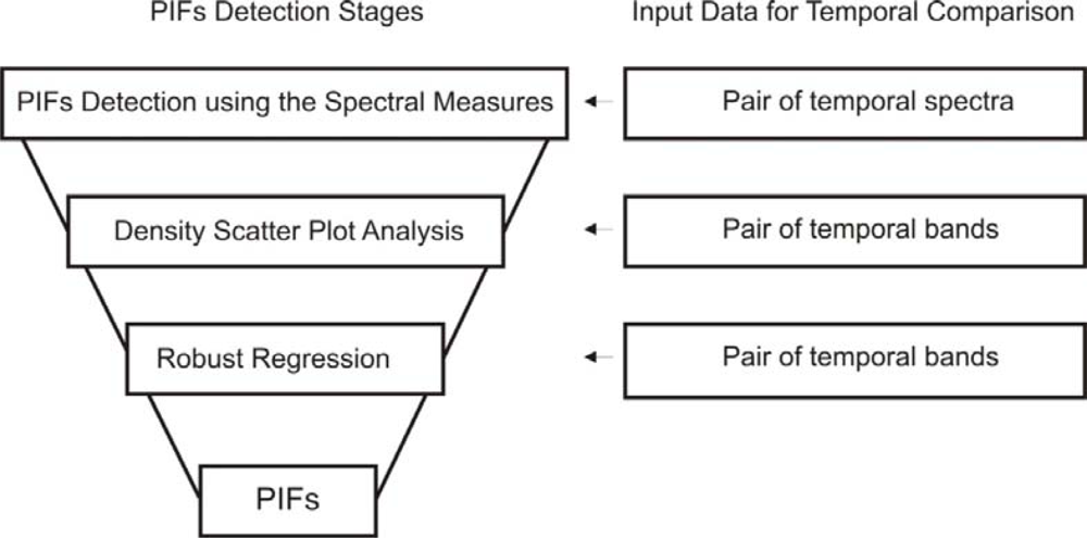
In this study, a new algorithm is formulated for radiometric normalization that combines three methods for the detection of PIFs: similarity and distance measures, a density scatter plot method, and robust linear regression. The methods presented are complementary and can be used together in consecutive steps that improve the selection of PIFs. The method was implemented in software developed in C++.

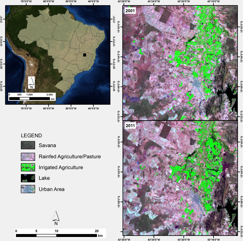
The proposed methods have been applied in an extensive irrigation project located in the Gorutuba region, Central Brazil. The irrigation project has established an important economic growth vector to agricultural activities and agro-industries, keeping the production under a high climate risk. The São Francisco River provides a steady water flow for use in irrigated farming. The topography is generally very flat, which favors the development of agriculture irrigation, involving the establishment of dikes and regulations. The agriculture irrigated produces mainly fruits; species include banana, pineapple, and mango. Thus, this area is suitable for this study because it presents different targets such as: lake, city, cultivated area, and natural vegetation.

2. Methods

The automatic radiometric normalization consists of the following steps: co-registration of the temporal images, selection of the PIFs, and linear regression from the PIFs. In this paper, the algorithm for the automatic detection of the PIFs combines methods that provide a gradual selection (Figure 2). Initially, the method performs a spectral analysis in time, using similarity and distance measurements, followed by band comparison from the density scatter-plot analysis, and finally a robust regression to eliminate possible outliers. Thus, each one of these methods was used to sequentially eliminate change points and create invariant point sets to achieve the radiometric normalization of the temporal images.

2.1. Image Acquisition and Preprocessing

The method considers, as inputs, two co-registered temporal images with their three dimensions: X, Y, and Z (spectral profile) acquired in the same geographical area at two times (t1 and t2). In the present paper, Landsat TM (Thematic Mapper) images are used. These were acquired without clouds during the same month of sequential years (9 September 2001, and 21 September 2011) in order to minimize any differences in sun angle and vegetation growth stage (Figure 3). Images have a size dimension of 1,000 × 1,000 pixels.

The images were co-registered from twelve ground control points identified in each image using ENVI software. The warping method used was the first-order polynomial (simplest method) combined with the nearest-neighbor resampling method to avoid interference in the pixel spectrum. The root mean squared error (RMS) value reported by ENVI was <0.2 pixels. Images have to be superimposed within 0.2 pixels (RMS) to achieve an error of only 10% [28,29]. Normalization was conducted by using the 2011 TM scene as the reference image to adjust the 2001 image. In radiometric normalization, the determination of reference and unnormalized variables is arbitrary, since both variables have measurement uncertainty associated with them, and the purpose is to convert them to a common scale. The importance of the reference image increases when the radiometric normalization is performed for a large amount of image over time, because all other images are adjusted to it. Thus, the choice of the reference image may be the best visual quality as well as the larger range of values, so that the information can be maintained as much as possible [30].

2.2. Pixel-by-Pixel Methods

2.2.1. Spectral Measures from the Original Images

The PIFs can be determined by distance and similarity measures between the spectra of images with the same spatial position at different times [25,26]. The main similarity measures used in the spectral classification are: cosine correlation used in the Spectral Angle Mapper (SAM) [31] and Pearson’s correlation coefficient used in the Spectral Correlation Mapper (SCM) [32], while the main distance measure utilized is Euclidean distance used in the minimum distance.

Table 1. Spectral Measures in Temporal Analysis.

Measures	Formulation	Characteristics
Euclidean Distance for change detection (EDCD)	${\mathit{ED}}_{\mathit{CD}}=\sqrt{\sum _{i=1}^N{\left(X_i^{t_1}-X_i^{t_2}\right)}^2}$	Sensitive to offset and gain factor
Spectral Angle Mapper for change detection (SAMCD)	${\mathit{SAM}}_{\mathit{CD}}=\alpha ={\mathit{cos}}^{-1}\frac{{\sum }_{i=1}^{i=N}{X}_i^{t_1}{X}_i^{t_2}}{\sqrt{{\sum }_{i=1}^{i=N}{\left(X_i^{t_1}\right)}^2{\sum }_{i=1}^{i=N}{\left(X_i^{t_2}\right)}^2}}$	Negative correlation is not detected Invariant to gain factor
Spectral Correlation Mapper for change detection (SCMCD)	${\mathit{SCM}}_{\mathit{CD}}=\frac{{\sum }_{i=1}^{i=N}\left(X_i^{t_1}-\overline{X^{t_1}}\right)\left(X_i^{t_2}-\overline{X^{t_2}}\right)}{\sqrt{{\sum }_{i=1}^{i=N}{\left(X_i^{t_1}-\overline{X^{t_1}}\right)}^2{\sum }_{i=1}^{i=N}{\left(X_i^{t_2}-\overline{X^{t_2}}\right)}^2}}$	Negative correlation is detected Invariant to offset and gain factor

shows the use of the measures in change detection (CD), considering the pixel X for the first (t₁) and second (t₂) times. The variable “i” corresponds to the spectral band and ranges from 1 to the number of bands (N).

The spectral measures provide different information about the target. This is because each measure has its own characteristics, which justifies the use of different measures in accordance with the spectral behavior and data type [26]. The ED_CD is sensitive to the bias (additive) factor and gain (multiplicative) factor. SAM_CD is unable to detect negatively correlated data and invariant to bias factors. SCM_CD is invariant to the bias and gain factors, and may be used with anti-correlated data. Values range from −1 to 1, where 1 means identical spectra, 0 means they are completely uncorrelated, and −1 means they are perfect opposites. The SCM_CD is therefore insensitive to illumination effects and is appropriate for eliminating shadows. The major difference between the correlation methods is that SAM_CD uses primary values for X^t₁ and X^t₂, whereas SCM_CD uses data centered by the means $\overline{X^{t_1}}$ and $\overline{X^{t_2}}$. Thus, the cosine correlation is equivalent to the uncentered version of Pearson’s correlation, assuming the population mean is zero.

The spectral measures can be combined in PIF detection, increasing efficiency. Thus, the user can choose the number of spectral measures to be used in PIF detection. PIF selection is only performed if the values are consistent with the thresholds of each method.

2.2.2. Distance Measures from the Canonical Variates

CCA was developed by Hotelling [33], and measures the linear relationship between two multidimensional variables. This multivariate analysis differs of the other transformation methods that identify the patterns of relationship within a single set of data. This characteristic has special emphasis in bi-temporal change detection, in which data consist of two sets of bands acquired at different times. CCA identifies image patterns common to both times, as well as patterns particular to each time. In this way CCA establishes a relationship of a set of predictor variables (V₁, V₂, …, V_n) from a set of criterion variables (Y₁, Y₂, …, Y_n), trying to find two sets of basis vectors (a and b), such that the correlations between the projections of the variables onto these basis vectors are mutually maximized [34].

$$a_1{Y}_1+a_2{Y}_2+\cdots +a_{\mathit{nb}}{Y}_{\mathit{nb}}=b_1{V}_1+b_2{V}_2+\cdots +b_{\mathit{nb}}{V}_{\mathit{nb}}$$

(1)

This approach is a complement of the multiple regression method that establishes a relationship of a set of predictors (V₁, V₂, ..., V_n) for a single criterion variable (Y). The calculation of the two sets of basis vectors (W_X^t1 and W_X^t2) can be obtained from the total covariance matrix (Cov) considering the two temporal variables X^t1 and X^t2 with zero mean:

$$Cov=\left(\begin{array}{ll}Co{v}_{X^{t_1}{X}^{t_1}}\hfill & Co{v}_{X^{t_1}{X}^{t_2}}\hfill \\ Co{v}_{X^{t_2}{X}^{t_1}}\hfill & Co{v}_{X^{t_2}{X}^{t_2}}\hfill \end{array}\right)$$

(2)

where Cov_X^t1X^t1 and Cov_X^t2X^t2 are the within-sets covariance matrices of X^t₁ and X^t₂ respectively and ${\mathit{Cov}}_{X^{t_1}{X}^{t_2}}=Co{v}_{X^{t_2}{X}^{t_1}}^T$ is the between-sets covariance matrix. The maximum of correlation (ρ) to W_X^t1 and W_X^t2 is the largest canonical correlation. Thus, the canonical correlations between X^t₁ and X^t₂ can be found by solving the eigenvalue equations:

$$Co{v}_{X^{t_1}{X}^{t_1}}^{-1}Co{v}_{X^{t_1}{X}^{t_2}}Co{v}_{X^{t_2}{X}^{t_2}}^{-1}Co{v}_{X^{t_2}{X}^{t_1}}={\rho }^2{W}_{X^{t_1}}$$

(3)

$$Co{v}_{X^{t_2}{X}^{t_2}}^{-1}Co{v}_{X^{t_2}{X}^{t_1}}Co{v}_{X^{t_1}{X}^{t_1}}^{-1}Co{v}_{X^{t_1}{X}^{t_2}}={\rho }^2{W}_{X^{t_2}}$$

(4)

where the eigenvalues ρ² are the squared canonical correlations and the eigenvectors W_X^t1 and W_X^t2 are the normalized canonical correlation basis vectors. The canonical variates (CV) are calculated by multiplying eigenvectors with the original images (X) for the first (t₁) and second (t₂) times subtracted by its means (μ) [34]:

$$C{V}^{t1}=W_{X^{t_1}}^T\cdot \left(X^{t_1}-{\mu }^{t_1}\right)$$

(5)

$$C{V}^{t2}=W_{X^{t_2}}^T\cdot \left(X^{t_2}-{\mu }^{t_2}\right)$$

(6)

Each pair of bands is orthogonal and independent of all other bands derived from the same data set. Successive pairs of canonical variates are based on residual variance. The first pair of canonical variates demonstrates the highest intercorrelation, the next pair, the second-highest correlation, and so forth. Thus, canonical correlation is an appropriate and powerful multivariate technique for both multiple dependent and independent variables. In this paper, the algorithm for the calculation of canonical variates, developed by Borga [34], was adapted for remote sensing images. This algorithm performs an ordering of canonical variates according to their eigenvalues.

Nielsen et al.[35] proposed the Multivariate Alteration Detection (MAD) technique, a change-detection method based on CCA. In MAD, the respective Canonical Variates (CVs) of the two times are subtracted in order to emphasize the changes:

$$\mathit{MAD}={\mathit{CV}}^{t2}-{\mathit{CV}}^{t1}$$

(7)

Therefore, MAD analysis takes the difference between linear combinations of the original data that have maximal correlation; it consists in normalization for a change detection scheme.

Spectral distance metrics can be calculated from temporal CVs. Canty et al.[27] used the square of the Normalized Euclidean Distance (NED²) between pixels of canonical variates to PIF detection:

$${\mathit{NED}}^2=\sum _{i=1}^N{\left(\frac{{\mathit{MAD}}_i}{{\sigma }_{{\mathit{MAD}}_i}}\right)}^2$$

(8)

However, this formulation can provide extremely high values that prevent the display of the distance image (rule-image). In this paper, we consider the Normalized Euclidean Distance (NED) more appropriate to image comparison with the other methods. NED is a simplification of the Mahalanobis Distance.

NED application in the magnitude of MAD images creates an ellipsoidal distribution that best represents the probability distribution of the estimated set by standardization of canonical variates. However, spectrum standardization is not always desired. CCA provides an ordering of image quality (according to its eigenvalues), where the uncorrelated noises with equal variance ( ${\sigma }_N^2$) are concentrated in the last components (decreasing Signal/Noise ratio). The use of all bands provides an increase of magnitude of noise components resulting in signal degradation and interference in the PFI detection. Thus, we propose that the user chooses the canonical variates to be used in calculating the distance, in order to eliminate noise components.

NED is not independent of the scene because its formulation uses the standard deviation (dependent of the scene). This characteristic differs from other measures; which consider only operations restricted to a given pixel; regardless of the size and value of the other pixels [26].

2.3. Band-by-Band Methods

2.3.1. Ridge Method

Scatter-plot analysis is a powerful approach to exploratory multivariate data analysis. Song et al.[20] identifies PIFs using scatter plots between bi-temporal images. However, the remote-sensing datasets are usually large, demanding additional procedures such as density representation and subset selection. In this work, the density representation is obtained by encoding the density values for a grey-scale image as 8-bit integers. The scatter plot can thus be represented by a 256 × 256 matrix. The transfer function from density values to gray-scale, or to pseudo-color can be manipulated through the color lookup table.

2.3.2. Robust Statistical Method

The mathematical model that best describes the normalization bi-temporal images involves linear regression of the PIFs. The algorithm assumes that the PIFs at t₂ are linearly related to the pixels at t₁. This implies that the spectral reflectance properties of the sampled pixels have not changed over time.

$$\mathit{Ref}=a+b\times \mathit{Sub}$$

(9)

where “Ref” is the reference image, “Sub” is the subject image, “a” is the linear coefficient, and “b” is the angular coefficient. The regression procedure is applied separately for each image band, therefore for a Landsat TM scene, six different equations are defined. However, statistical fluctuations may be caused by the presence of outliers. Regression analysis or least-squares estimation are highly susceptible to outliers, which can generate erroneous values for slope and intercept, and consequently lead to false conclusions. In this regard, the robust statistical methods are suitable to eliminate outliers considering a model that explains the greater part of the data. Thus, robust regression determines the PIFs in the presence of noise (outliers), which is important for the radiometric normalization [18,19,36]. However, errors can occur if the invariant targets do not represent the greater part of the scene. In this paper the robust regression is a refinement stage that considers a prior selection of PIFs by spectral measures and density scatter plots.

Several estimators have been developed in order to be insensitive to small deviations from an idealized assumption for straight-line fit [23,24]. Maximum-likelihood arguments (M-estimates) are usually the most relevant for model-fitting. In this work we adopted the numerical calculation of M-estimates described by Press et al.[37]. These estimators minimize the sum of a symmetric, positive-definite function f(r_i), where r_i are residuals, i.e., difference between the data point and the fitted value [38]. Several functions have been proposed in order to reduce the influence of large residual values on the estimated fit [23,39,40]. In this work we adopted the numerical calculation of M-estimates described by Press et al.[37]. For more details about the theory and application of M-estimators, see [23,37,41,42].

2.4. Optional Use of a Mask

Optionally, targets with high susceptibility to change over time can be disregarded as being unreliable, such as vegetation. The removal of these targets should be made by use of a binary mask, which includes the value of 1 in the analysis and ignores the value of 0. Thus, undesirable targets may be disposed even with spectral and density measures compatible with a PIF.

2.5. Radiometric Normalization Accuracy

Greater accuracy implies more similarity between the frequency distribution of reference and normalized data, i.e., similar values of mean and dispersion measures. Therefore the comparison of these statistical measures in PIFs areas is widely used for radiometric normalization accuracy, since this procedure depends only on the resulting images. The main statistical indices are measures of central tendency (mean) and dispersion (range, standard deviation, variance, and coefficient of variation) between reference and normalized images and linear regression information (root-mean-square error and correlation coefficient) [27,30].

However the sample size has a significant impact on the statistical results. A smaller sampling of PIFs regularly gives better performance because it reduces noise and outliers, which can substantially degrade the radiometric normalization. Variations in the number of samples modify the statistical data for the same method. Therefore, the comparison of methods must use the same number of pixels in order to eliminate this effect. In the present study, we developed a program that considers three alternatives for the PIFs selection from distance or similarity images (pixel-by-pixel methods): threshold values of the spectral measures, number of pixels, and image percentage (all user-defined).

These statistical procedures, despite being widely used should be evaluated carefully, since they represent the linear regression fits, and not directly the quality of PIFs. The comparison of the spectral behavior of known targets is still the most straightforward way to judge the overall performance of the radiometric normalization methods.

3. Results

3.1. Results of the Pixel-by-Pixel Procedures

3.1.1. Distance and Similarity Measures from Original Images

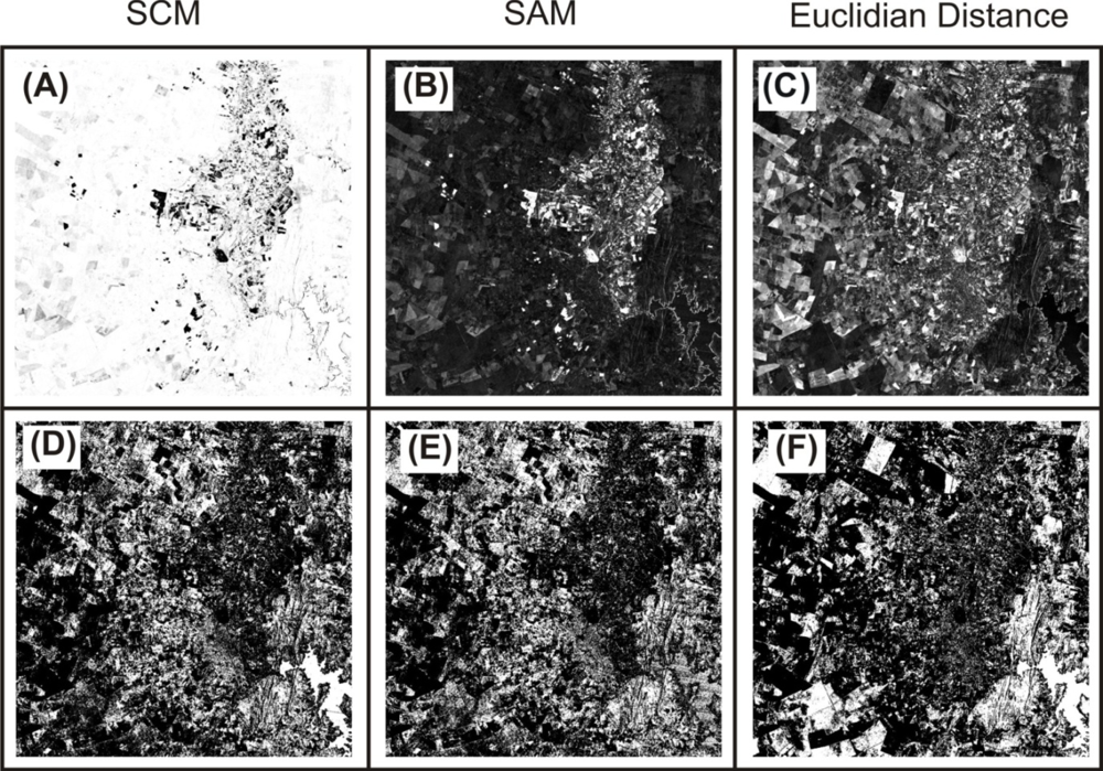
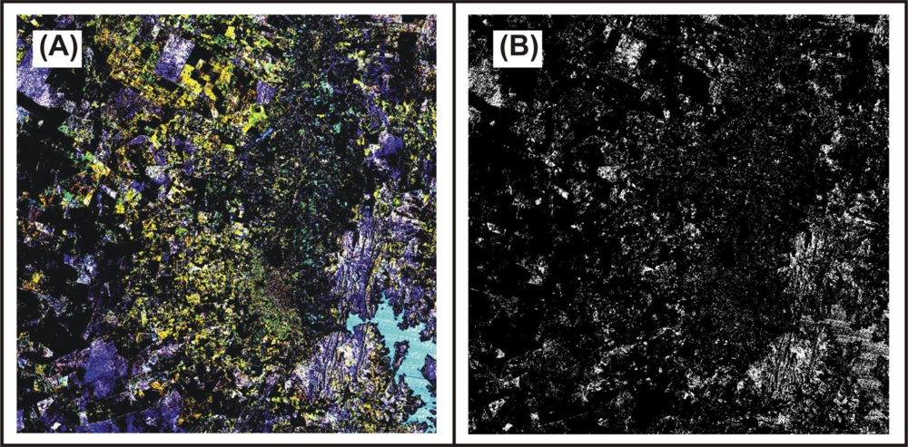
Initially, the PIFs detection using different spectral measures from original images were evaluated. Figure 4 shows the spectral measure images in a gray-scale format and PIF images in a binary format. The SCM_CD image (Figure 4(a)) shows the most likely invariant points as bright, while the SAM_CD and distance images (Figure 4(b,c)) show them as dark. A PIF selection with less points should adopt a threshold with a high value to the SCM_CD method; low angles from SAM_CD, and low ED_CD values. As an example, a threshold value of 20% (200,000 pixels) was evaluated for the study area. PIFs identified with them are represented with bright colors for each of the three approaches (Figure 4(d–f)). The PIFs have been well distributed in the image considering the different targets of the scene.

Most of the invariant points are identified independently using the three different measures; however there are differences among the results and these can be visualized from the intersection PIFs among the methods (

Table 2. Intersection number of PIFs from different methods (SCM_CD, SAM_CD, and ED_CD) considering a threshold value of 20%.

	SCMCD (20%)	SAMCD (20%)	EDCD (20%)
SCMCD(20%)	200,000	160,398	106,981
SAMCD(20%)	160,398	200,000	102,774
EDCD(20%)	106,981	102,774	200,000

). The most pronounced differences occur between the similarity measures and Euclidean distance, where nearly half of the PIFs are coincidental. The SAM_CD and SCM_CD show a high PIFs overlap, i.e., approximately 80% of pixels.

The spatial location of PIFs from the different methods can be performed by color composite images (Figure 5(a)). In the color composite, the invariant points identified by all three methods are white, and change points are black. Primary colors (red, green, and blue) indicate identification by a single method; secondary colors (cyan, magenta, and yellow) indicate identification by two methods. The similarity measures (SCM_CD and SAM_CD) have greater amounts of common invariant points (yellow color). Figure 5(b) shows a PIF image with the intersection of all methods, where the PIFs are represented with bright colors.

Figure 6 shows an example of the differences between the spectral measures of similarity and distance. In Figure 6(a) two temporal spectra that have the same shape and offset difference are identified as invariant point using the SAM_CD and SCM_CD measures, and as a change point by the ED_CD. In contrast, Figure 6(b) demonstrates two temporal spectra identified as invariant point using the Euclidean distance, and as a change point by the SAM_CD and SCM_CD measures. These differences emphasize that the methods are complementary and their combinations allow a greater constraint for PIFs and a significant number of the pixels are change targets between the temporal images (Figure 6(b)).

Statistical data from the simple linear regression for the selected PIFs are compared in order to evaluate the different spectral measures (

Table 3. Least squares regression on training PIFs (200,000) from SCM_CD, SAM_CD, and ED_CD measures; α is the fitted intercept, β is the fitted slope, root-mean-square errors (RMSE) is the root mean squared error and R is the correlation coefficient.

Bands	SCMCD				SAMCD				EDCD
	α	β	RMSE	R	α	β	RMSE	R	α	β	RMSE	R
Band-1	−7.33	1.114	5.437	0.865	−3.316	1.061	5.121	0.851	−0.869	0.99	2.805	0.93
Band-2	−3.679	1.162	4.220	0.905	−3.073	1.143	3.901	0.902	0.248	1.006	1.988	0.959
Band-3	−3.675	1.144	6.615	0.944	−2.547	1.122	6.307	0.93	−0.263	1.026	3.254	0.977
Band-4	−0.025	1.097	6.642	0.964	2.352	1.066	6.454	0.94	2.518	1.037	4.462	0.98
Band-5	−1.345	1.06	11.398	0.974	−1.315	1.068	11.688	0.954	2.539	0.991	5.086	0.993
Band-7	−0.149	1.076	6.642	0.968	0.128	1.076	6.846	0.948	2.026	0.989	3.582	0.986

,

Table 4. Comparison of mean intensities of hold-out test PIFs (20%) for the three PIF methods using the 2001 scene before and after normalization to the 2011 scene with least squares regression.

SCMCD
	Band 1	Band 2	Band 3	Band 4	Band 5	Band 7
Uncorrected (2001)	76.461	38.203	51.968	64.288	126.890	59.212
Normalized (2001)	77.273	40.199	55.236	69.964	132.700	63.073
Reference (2011)	77.830	40.713	55.783	70.484	133.170	63.540
Difference	0.550	0.513	0.546	0.520	0.465	0.466
SAMCD
	Band 1	Band 2	Band 3	Band 4	Band 5	Band 7
Uncorrected (2001)	77.189	38.927	54.111	66.257	132.930	62.097
Normalized (2001)	78.030	40.927	57.686	72.463	140.140	66.420
Reference (2011)	78.546	41.431	58.182	72.987	140.630	66.921
Difference	0.516	0.504	0.495	0.523	0.491	0.500
EDCD
	Band 1	Band 2	Band 3	Band 4	Band 5	Band 7
Uncorrected (2001)	72.809	34.229	44.099	56.736	108.240	48.797
Normalized (2001)	70.809	34.229	44.412	60.840	109.33	49.791
Reference (2011)	71.224	34.680	44.977	61.367	109.840	50.271
Difference	0.414	0.4505	0.564	0.527	0.503	0.480

and

Table 5. Comparison of dispersion measures of hold-out test PIFs (20%) for the three measures (SCM_CD, SAM_CD and ED_CD) using the 2001 scene before and after normalization to the 2011 scene with least squares regression.

SCMCD
		Band 1	Band 2	Band 3	Band 4	Band 5	Band 7
Variances	Uncorrected (2001)	70.69438	59.44261	273.3577	480.6458	2131.235	562.5406
	Normalized (2001)	88.19824	79.76944	358.481	581.9668	2387.68	646.6398
	Reference (2011)	117.2427	98.06528	401.5877	622.2835	2524.955	694.9333
Range	Uncorrected (2001)	78	62	113	148	253	143
	Normalized (2001)	87	72	129	162	255	153
	Reference (2011)	99	73	128	148	255	163
Coefficient of	Uncorrected (2001)	0.109965	0.201812	0.318149	0.341022	0.363826	0.400559
	Normalized (2001)	0.121536	0.22218	0.342774	0.344807	0.36822	0.403169
	Reference (2011)	0.139135	0.243237	0.359244	0.353919	0.377336	0.414881
SAMCD
		Band 1	Band 2	Band 3	Band 4	Band 5	Band 7
Variances	Uncorrected (2001)	61.32971	50.99061	203.6081	275.8851	1223.483	361.7351
	Normalized (2001)	69.58914	66.44938	256.8769	315.0233	1392.437	418.5648
	Reference (2011)	95.20167	81.86585	296.2384	355.2058	1531.65	465.3757
Range	Uncorrected (2001)	133	84	127	145	252	140
	Normalized (2001)	141	96	142	155	254	150
	Reference (2011)	99	72	117	138	255	162
Coefficient of	Uncorrected (2001)	0.101456	0.183442	0.263701	0.250687	0.263134	0.306285
	Normalized (2001)	0.106908	0.199176	0.277837	0.244937	0.266286	0.308022
	Reference (2011)	0.124221	0.218387	0.295823	0.258223	0.278294	0.32236
EDCD
		Band 1	Band 2	Band 3	Band 4	Band 5	Band 7
Variances	Uncorrected (2001)	51.63264	44.39962	208.6694	451.3844	1791.989	443.5186
	Normalized (2001)	51.6276	44.39962	219.4595	488.523	1768.854	441.4567
	Reference (2011)	58.49063	48.87633	230.1959	505.5454	1786.699	446.3774
Range	Uncorrected (2001)	91	65	113	148	253	140
	Normalized (2001)	90	65	115	154	251	138
	Reference (2011)	99	69	119	141	254	135
Coefficient of	Uncorrected (2001)	0.098691	0.194667	0.327568	0.374467	0.391084	0.431584
	Normalized (2001)	0.101473	0.194667	0.333561	0.363291	0.384677	0.421984
	Reference (2011)	0.107378	0.201592	0.337334	0.36639	0.384839	0.420275

). A comparison of the spectral measures adopted a simple linear regression to avoid interference from other methods (ridge and robust regression).

Table 3 gives the corresponding information about regression statistics. PIFs-ED_CD shows the best-fit linear regressions for all bands with the lowest root-mean-square errors (RMSE) and highest correlation coefficients (R). This behavior was expected because the minimum Euclidean distance tends to be more aligned to a straight line; unlike the similarity measures that can have greater variability. PIFs-SCM_CD provides better correlation coefficients than the PIFs-SAM_CD, however the PIFs-SAM_CD presents best RMSE values.

Table 4 shows the means of the 2011 scene (reference image) and 2001 scenes, before and after normalizations, using least squares regression line. The differences between the means of reference and normalized images are always close to 0.5. SCM_CD has the lowest average differences for the infrared bands (4,5,7). SAM_CD shows a lowest difference value for band 3, while the ED_CD for bands 1 and 2.

Measures of dispersion differ among PIFs from ED and measures of similarities (SCM and SAM) (Table 5). The PIFs from ED have lower differences of variance and coefficient of variation between the reference image and the images uncorrected and corrected. These measurements, between SAM and SCM are similar, but SAM presents variance values closest between the reference image and the normalized image, whereas SCM shows variation coefficients, which are slightly closer. The range of values varies greatly although the SCM and ED present more homogeneous values than the SAM.

3.1.2. Distance Measures from Canonical Variates (CVs)

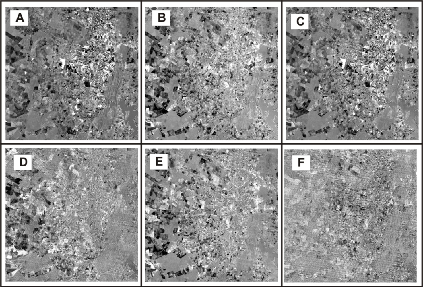
MAD components have an ordering image that highlights the reduction of intercorrelation between the CV pairs and increased noise interference (Figure 7). The last component concentrates the noise fraction (Figure 7(f)).

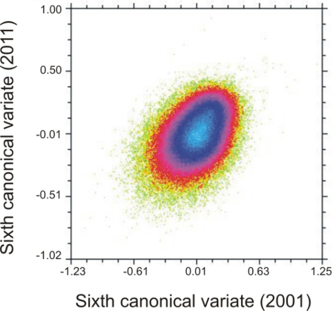
The scatterplot between the pair of the latest CV-pair appears spherically distributed around the data. This is evidence of the predominance of the uncorrelated noises with equal variance in all bands (Figure 8). This optimal ordering of image quality (when the noise variances in all bands are equal) is similar with the standard principal components transformation. However, CCA transformation is not suitable for other types of spatial noise, such as salt-and-pepper noise. The amount of noise reduction depends on the degree of temporal-band correlation, the relative noise in each input band, and the type of noise performed on the transformed components.

The high correlation frequently exists in multi-temporal data provides a redundancy reduction and increasing the signal magnitudes in the first CVs. Once data have been transformed into canonical variates with decreasing noise, the subsequent calculation of the distance measures between the temporal variables can disregard the noisiest components. This practice should be emphasized with the use of the NED or Mahalanobis distance that lead to data normalization, i.e., MAD components are converted to a common scale (standard deviation equal to 1). Noise bands that have smaller value range (Figure 9), with the use of NED are amplified in comparison with other bands.

In this work we calculated the NED measures considering two scenarios: with all MAD components and removing the noisy components. The NED² image originally described by Canty [27] is not shown due to interference from very high values and because the PIF result is equal to the NED considering a same threshold by image percentage. Figure 10 demonstrates the NED-MAD images and its PIFs images (20%) considering: all bands, first five MAD components, and first three MAD components.

Table 6. Number of PIFs from the intersection of different methods considering a threshold value of 20%: NED-MAD using all bands, NED-MAD using first five components, NED-MAD using first three components, SCM_CD, SAM_CD and ED_CD.

	NED-MAD	NED-MAD	NED-MAD	SCMCD	SAMCD	EDCD
	(All Bands)	(5 Bands)	(3 Bands)
NED-MAD (all bands)	200,000	160,923	139,654	52,188	59,408	26,246
NED-MAD (5 bands)	160,923	200,000	155,799	47,496	55,353	14,738
NED-MAD (3 bands)	139,654	155,799	200,000	52,204	59,901	17,874

shows the number of similar PIFs among the NED-MAD images (considering different amounts of MAD components) and spectral measures applied to original images (SAM, SCM, and ED). PIFs from NED-MAD, using all components, have an overlap of approximately 80% (160, 923 pixels) with the PIFs using five MAD components, and around 70% (139,654 pixels) with the PIF using three MAD components.

The number of coincident PIFs from the spectral measures (SCM, SAM, and ED) using the original images and the NED using the MAD components are extremely low, indicating a significant difference between the two procedures (Table 6). The smaller intersections are among the PIFs from ED and NED-MAD. PIFs from the similarity measures (SCM and SAM) have an overlap of approximately 25% (50,000 pixels) with the PIFs from NED-MAD.

Table 7. Least squares regression on training PIF pixels (200,000) from the NED-MAD using all bands, NED-MAD image using first five components, NED-MAD using first three components; α is the fitted intercept, β is the fitted slope, RMSE is the root mean squared error and R is the coefficient correlation.

	NED-MAD (All Components)				NED-MAD (Five Components)				NED-MAD (Three Components)
Bands	α	β	RMSE	R	α	β	RMSE	R	α	β	RMSE	R
Band-1	−3.513	1.072	2.314	0.945	−2.249	1.057	2.190	0.955	−0.792	1.039	1.856	0.968
Band-2	−0.469	1.128	1.721	0.967	0.563	1.104	1.607	0.973	1.439	1.079	1.578	0.974
Band-3	3.086	1.100	2.792	0.972	4.598	1.075	2.789	0.976	4.774	1.065	3.697	0.962
Band-4	13.533	0.983	3.646	0.962	14.757	0.967	3.594	0.961	18.918	0.888	5.929	0.913
Band-5	13.163	1.002	7.158	0.963	15.295	0.990	6.986	0.965	15.875	0.983	6.160	0.975
Band-7	5.482	1.038	4.053	0.966	8.028	1.004	5.218	0.945	8.203	1.002	5.066	0.952

shows the fitted intercepts, slopes, correlation coefficient and RMSE for least squares regression on the 200,000 PIFs from NED-MAD images. The removal of the noisiest component provides the best fit regression line, with higher correlation coefficient and lower RMSE for all bands, except for band 7. Thus, the noise reduction provides a more homogeneous PIF selection. In opposition, PIF from NED using only the first three MAD components causes a loss of signal, decreasing the fits of regression lines for bands 3, 5, and 7.

PIFs from NED-MAD compared to PIFs from ED_CD exhibit higher correlation coefficients for linear regression in the first and second bands and the lower for the rest. An inverse behavior is found for the RMSE values, where PIFs from NED-MAD presents lower values for bands 1, 2, 3, and 4. PIFs from NED-MAD show best fit regression line compared to the two similarity measures (SCM_CD and SAM_CD) applied to the original images.

Table 8. Comparison of mean intensities of hold-out test PIFs (20%) for the NED-MAD method (all, 5, and 3 components), considering 2001 scene before and after normalization to the 2011 scene with least squares regression.

NED-MAD (All Bands)
	Band 1	Band 2	Band 3	Band 4	Band 5	Band 7
Uncorrected (2001)	73.53389	34.98043	47.22892	59.63658	120.6294	54.58548
Normalized (2001)	74.80974	38.51939	54.49465	71.60842	133.6294	61.72854
Reference (2011)	75.29658	38.97923	55.02094	72.13204	134.0009	62.14728
Difference	0.48684	0.45984	0.526285	0.52361	0.37149	0.41874
NED-MAD (5 Bands)
	Band 1	Band 2	Band 3	Band 4	Band 5	Band 7
Uncorrected (2001)	74.54509	35.99552	49.202	61.24536	125.102	57.13146
Normalized (2001)	75.96249	39.72751	56.94335	73.55464	138.619	65.13146
Reference (2011)	76.55546	40.28415	57.46744	73.98557	139.0883	65.3966
Difference	0.59298	0.55665	0.524095	0.430935	0.46925	0.265145
NED-MAD (3 Bands)
	Band 1	Band 2	Band 3	Band 4	Band 5	Band 7
Uncorrected (2001)	74.39065	36.0114	49.06649	63.04542	124.0779	56.60791
Normalized (2001)	75.96621	39.70047	56.54078	74.37767	137.4494	64.60791
Reference (2011)	76.50336	40.29939	57.02833	74.90395	137.8846	64.93313
Difference	0.53715	0.59892	0.487555	0.526275	0.43518	0.32522

shows the means of PIFs from the NED-MAD method considering all-components, first five components and first three components for the 2011 scene (reference image) and 2001 scene before and after normalizations using least squares regression line. The differences between the means of reference and normalized images are always close to 0.5.

The NED-MAD, considering all the bands, shows the smallest differences for bands 1, 2, and 5. However, the differences of the means of PIFs from NED-MAD procedures are larger in all bands compared to PIFs from EDCD (Table 4).

Table 9. Comparison of dispersion measures of hold-out test PIFs (20%) for the three PIF methods using the 2001 scene, before and after normalization, to the 2011 scene with least squares regression.

NED-MAD (All Bands)
		Band 1	Band 2	Band 3	Band 4	Band 5	Band 7
Variances	Uncorrected (2001)	39.29503	33.80525	126.7082	171.6435	651.4781	210.9658
	Normalized (2001)	44.91777	43.05102	153.9639	169.1287	651.4781	225.548
	Reference (2011)	50.49108	45.95556	162.0483	179.015	704.9602	243.7734
Range	Uncorrected (2001)	60	58	95	133	238	139
	Normalized (2001)	64	66	105	131	238	144
	Reference (2011)	64	59	101	131	237	148
Coefficient of Variation	Uncorrected (2001)	0.085247	0.166214	0.238339	0.219685	0.211591	0.26609
	Normalized (2001)	0.089588	0.170338	0.227696	0.181612	0.191006	0.243295
	Reference (2011)	0.09437	0.173915	0.231363	0.185488	0.198141	0.25123
NED-MAD (5 bands)
		Band 1	Band 2	Band 3	Band 4	Band 5	Band 7
Variances	Uncorrected (2001)	44.14236	37.52932	137.2826	167.8967	671.9878	223.6594
	Normalized (2001)	50.42474	46.9415	158.6868	156.1622	650.1234	223.6594
	Reference (2011)	54.12543	48.28298	166.2875	169.9436	706.807	252.7447
Range	Uncorrected (2001)	63	58	100	124	238	131
	Normalized (2001)	66	64	108	120	235	131
	Reference (2011)	68	59	104	126	238	132
Coefficient of Variation	Uncorrected (2001)	0.089127	0.170191	0.238136	0.211567	0.207213	0.261769
	Normalized (2001)	0.093481	0.17246	0.221222	0.169894	0.18394	0.229616
	Reference (2011)	0.0961	0.17249	0.224392	0.1762	0.191144	0.243101
NED-MAD (3 Bands)
		Band 1	Band 2	Band 3	Band 4	Band 5	Band 7
Variances	Uncorrected (2001)	47.69037	39.2796	150.0455	222.4742	760.6277	249.8103
	Normalized (2001)	53.1722	46.57776	169.1822	175.7566	735.9215	249.8103
	Reference (2011)	54.9329	48.23015	183.8415	210.5953	773.4186	276.5494
Range	Uncorrected (2001)	68	60	126	143	244	133
	Normalized (2001)	71	65	134	127	240	133
	Reference (2011)	72	59	110	139	251	135
Coefficient of Variation	Uncorrected (2001)	0.092832	0.174038	0.249647	0.236585	0.222276	0.279208
	Normalized (2001)	0.095989	0.171907	0.230047	0.178243	0.197366	0.244636
	Reference (2011)	0.09688	0.17233	0.237756	0.19374	0.201693	0.256106

shows the dispersion measures of hold-out test PIFs for the three NED-MAD procedures. The variance and correlation coefficient between the reference and normalized image present the lowest differences distributed in different procedures: NED-MAD with all bands (bands 4 and 7); NED-MAD with the first 5 components (band 3), and NED-MAD with the first 3 components (bands 1, 2, and 5). The range of values shows greater differences for PIFs from NED-MAD using first three bands.

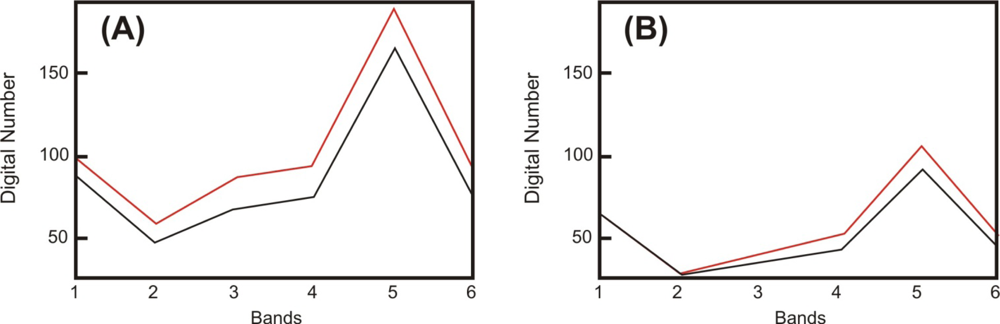
3.1.3. Spectral Analysis from the Dark Radiometric Control Target

Spectral analysis between the reference and normalized images was made from the dark radiometric control targets, considering water body. Dimension of the water body may be important, and small sizes may not be representative [12]. The present study adopted 55 pixels present in the center of the water body of a dam. Mean of the absolute deviations between the reference and normalized images demonstrates the adequacy of different measures in the PIF selection (Figure 11). Normalized data considering the SCM, SAM, and ED methods showed results very close to the reference data. The best result is obtained by using the SCM method followed by SAM and ED methods. In contrast, the normalized spectra considering the NED-MAD, method show the highest deviations (Figure 11).

Results show a different behavior of the fitting information of the linear regression model from PIFs, where for example the distance measures have lower RMSE values and higher R values (Tables 3 and 7). These apparently contradictory results can be explained. The distance measures (ED and NED) describe a deviation from an ideal condition where there is equality between the temporal spectra (null condition), i.e., a regression with a slope of 1 and intercept of zero. Therefore, the selection of pixels consider deviations from this ideal condition, even extending the limit of distance, and mismatches can occur. However, the distance measures by considering only values close to the ideal line (X^t₁ = X^t₂) always provide points fitted to straight line.

The similarity measures are not consistently related to the accuracy of the prediction, i.e., the degree to which the spectrum of time 1 approaches time 2. Statistically, SCM and partially SAM values are often unrelated to the sizes of the difference between the temporal spectra. The similarity measures are usually found to be a value that describes the quality or relative accuracy of the PIF samples. For example, the correlation is not affected by gain and offset effects, which makes high correlations possible even when the distance accuracy tends to be too weak or too strong. Thus, the similarity measures show a selection of points with larger dispersion measures. This feature allows the SCM to detect points without the restriction of an idealized model (α = 0 and β = 1). However, if the scattering is appreciable the line-fitting becomes subjective and unreliable. Therefore, the combined use of the two measures is the best solution.

The worst results for the NED-MAD measures are probably derived from the susceptibility of CCA to be influenced by the correlation of current changes in the ground target. CCA generates eigenvectors that describes the linear relations from the effects of atmosphere, illumination, and sensor calibration (that are external to the ground target). Temporal images with the majority of consistently changed ground targets generate eigenvalues conditioned to it, which interferes and modify the true PIFs, damaging their detection.

These results demonstrate that statistical data from the fits of the linear regression (RMS, correlation coefficient, and measures of central tendency and dispersion restricted to selected points) does not evidence necessarily the PIFs quality.

3.2. Results of the Band-by-Band Procedures

The use of ridge method on the previously selected PIFs allows a supplementary pixels reduction. Figure 12 shows scatter plots and PIF images for band 4 made using two density thresholds, 12 and 26. In order to emphasize the results of this method for the figure, the original data are regarded as input, rather than points previously selected using spectral measurements. The PIFs eliminated for each band can be viewed in binary images (Figure 12(d,e)).

One problem in density thresholds is the elimination of points having low density that are positioned along the line (ridge). These are usually points at each end of the ridge. Therefore, this processing step needs to be done carefully to avoid loss of relevant information. The pixels eliminated in a particular band can be eliminated in all five other bands.

The final step is to perform the robust regression for determining the line of best fit to the data from the reference and subject image for each image band. Robust regression procedure automatically omits eventual outliers in the calculations considering an absolute deviation value. The robust procedures fit the calibration line through the dark and bright targets. Figure 13 shows the robust approach based on M-estimation regarding all bands, considering 106 PIFs from intersection of SCM and ED methods. In practice, with a good set of targets from the previous methods, there is very little difference between the least squares and M-estimation calibration lines.

The proposed combination of methods enables one to extract points from various conditions that can be applied from image to image. Thus, areas labeled as invariant points in a method can be described as change point in the next methods. The method allows one to select a number of targets to cover the range from bright to dark data values. This highlights the importance of using difference techniques.

Statistical analyses of these complementary methods (ridge and robust regression), following pixel-by-pixel, always provide the best fit straight line since it eliminates outliers, making the demonstration unnecessary.

3.3. Program

The main functions of the program are organized in the main window interface, which contains the temporal image input boxes, mask image input box, spectral measures box, density scatter plot box, robust regression box, and image display (Figure 14).

Input files are required for the two temporal images (X^t₁ and X^t₂), which must be co-registered and have the same number of rows, columns, and bands. The first image is used as a reference while the second is the image to be corrected. The program reads general raster data stored as an interleaved binary stream of bytes in the Band Sequential Format (BSQ) and Band Interleaved by Pixel Format (BIP). Each image is accompanied by a header file in ASCII (text) containing information to read data file, such as: sample numbers, line numbers, bands, interleave code (BIP or BSQ), and data type (byte, signed and unsigned integer, long integer, floating point, 64-bit integer, and unsigned 64-bit integer). This configuration combining image and header file allows versatility in the use of different image formats. When the user tries to open an image without the header file, an interface requesting the necessary information about the input image structure automatically appears. Optionally, a binary mask can be used as an input file to disregard some variants targets over time.

Four options for the automatic detection of PIFs using spectral measures are provided: SCM, SAM, Euclidean distance, and NED-MAD. The user can select the measures and their threshold values. The program allows the user to select different spectral measures simultaneously. The PIFs are only selected if they meet all conditions set out in the spectral measures. The program allows a preview of PIF images, obtained by the spectral measures, facilitating the user to, if necessary, reset the threshold values.

The ridge method can be applied from pre-selected PIFs from the previous step. The density scatter plot can be visualized from the preview button, which opens a window interface for the ridge method (Figure 15).

In the scatter-plot density window, the user can choose to display the pair of bands and a pre-saved color table. At the bottom of the window, the user can set the density threshold value in order to eliminate the outliers. The elimination of the targets can be made by considering a single value for each pair of bands (multiple thresholds) or a single value for all scatter plots (single threshold). Density threshold value can be set with a scrollbar ranging from 0 to 255, derived by linear conversion of density values.

Finally, the robust regression using PIFs can be applied. In the main window the user can choose between the simple linear regression and robust regression from a check box. Thus, both method results can be compared. In the robust regression, the user must set the absolute deviation value between the regression line and the points in order to select the outliers. When the absolute deviation is greater than the set value, the observation is removed and the procedure is repeated. The decrease in the absolute deviation value by the user increases the number of outliers.

The linear regression window can be visualized with the preview button (Figure 16). The user must select the band and color table for the density scatter-plot window. Moreover, the program allows the visualization of the regression line and the distribution of its points. In the case of a wrong selection of points, the program allows the absolute deviation threshold to be modified. Once the threshold has been determined, the slope and intercept values are applied for each subject band, obtaining the calibrated images.

After the generation of calibrated images, the program generates statistics on the following images: reference, uncalibrated, and calibrated, considering the following statistical values: mean, variance, range, and coefficient of variation.

The program generates the following output files: radiometrically normalized images and PIF images. All inputs and results are shown in the File List, so it is possible to visualize them by choosing “Gray Scale” or “RGB” composite. The display interface provides basic functions for image visualization such as zoom areas and pixel values. Moreover, the results (output files) can be read with other images viewers.

4. Discussion

4.1. Comparison among Spectral Measures

The spectral measures can be performed on the original images, or on CVs from CCA. The use of CCA aims to correct temporal images (gain and offset). Thus CCA generates matrices of eigenvectors for both temporal sets that are invariants to linear and affine scaling, provided that the linear transformations are homogeneous for the entire image (such as band-by-band method). CCA operates throughout the bands; consequently specific effects in different parts of the image are not corrected. In addition, the calculation of eigenvectors in CCA is influenced, not only by the gain and offset from sensor-illumination-atmospheric effects, but also by systematic changes in the ground. Therefore, the contributions of other correlated attributes though the temporal bands (e.g., seasonal changes in vegetation, planting cycle) are difficult to determine due to mathematical formulation. The issue of the CCA application is to introduce a bias associated with correlations of surface changes to the true PIFs, hindering their detection. The canonical analysis (such as the principal components and factor analysis) should use images with a prevalence of unchanged targets. Moreover, CVs images have a spatial noise that should be considered in the calculation of the distance measures. The elimination of noisy components of CVs should be explored as an improvement to the method.

Spectral measures on the original temporal images consider both land cover changes as undesirable effects (e.g., different atmospheric conditions, variations in the solar illumination angles, and sensor calibration trends). Normally, the relative radiometric correction adopts the assumption that the linear effects are much greater than nonlinear effects [3,16,27]. In this case, SCM measure is completely invariant to linear transformations, even considering different behaviors on parts of the image. The use of distance measures on the pre-selected data by SCM measure enables the decrease the scattering data and outliers. Thus, combining similarity and distance measures on the original images have greater simplicity and control over the generated information.

Statistical data of the linear regression (RMSE, correlation coefficient, and measures of central tendency, and dispersion restricted to selected points) does not always describe the PIFs quality.

4.2. Advantages and Drawbacks of the Proposed Method

The present method integrates different radiometric normalization algorithms with distinct mathematical and statistical operations that provide a set of alternatives according to the characteristics of the data. The methods can be combined in different ways, not needing to use all available methods. Compared to some previous relative radiometric normalization methods, this new method offers several improvements and advantages because a single method cannot be used in all situations. The best combination of methods is to adopt a pixel-by-pixel method followed by the band-by-band method. Thus, PIFs selection accuracy is distributed in the different methods that provide a sequential selection, taking into account, not only, the statistical behavior of the samples but also their physical properties, such as surface moisture, shadow, etc.. This method can be used for the pre-processing of different multispectral images (e.g., ASTER, SPOT, CBERS, among others) concerning bi-temporal data with the same spectral bands and radiometric resolution. Radiometric normalization of panchromatic images can be done considering only ridge and robust regression methods. This relative normalization algorithm is wide-ranging and can be used for most operational applications, different images and conditions.

While this approach is straightforward and brings together different algorithms, it still shows problems, especially with the effects of heterogeneous aerosol scattering and water vapor content in a scene. All methods of PIFs detection presume a uniform behavior for atmospheric effects; being suitable for molecular scattering and absorption by ozone and oxygen because their concentrations are quite stable over both time and space. Contrary to this, most aerosols are heterogeneously distributed which makes this task more difficult and requires the development of new algorithms.

Furthermore, atmospheric effects on the two images can be different, not only spatially, but also in the spectral dimension damaging PIFs detection by pixel-by-pixel methods. Considering aerosol effects, a simple procedure is used with infrared bands that are less contaminated, in the specific case of TM/ETM+ imagery the bands 4, 5, and 7. However, this procedure is ineffective if there are thick aerosols and thin clouds. Therefore, a challenge in improving the methods of relative correction is the development of procedures to consider the heterogeneity of the image, i.e., specific linear regressions for different portions of the image.

5. Conclusion

The automatic selection of the invariant targets eliminates the need of a detailed manual comparison between each pair of the temporal image. PIFs detection from only band-by-band method show great limitations, requiring assume that the majority of the targets are invariant between a given image and the reference image. The improved efficiency of the band-by-band method is obtained by the association with pixel-by-pixel methods. Thus this paper proposes a new alternative to radiometric normalization between temporal images considering the combination of different procedures for automatic PIF selection. There is no one method that is better than others in every situation. Thus, the pixel-by-pixel approach (similarity and distance measures considering original image and Canonical Variates (CVs)) and band-by-band approach (density scatter plot and robust regression) should be used in conjunction to PIF estimation. This is because different methods have particular properties, some of which may be desirable for certain applications but not for others.

The combination of these methods provides a sequence of statistical techniques with independent criteria that provides the error minimization and best set of invariant targets. The sequential PIF selection obtains a number of invariant targets, which consider the entire brightness range of the images, ensuring the linear relationship between the image pairs during the calibration. The procedures described in this paper, still present limitations for nonlinear effects, which pose a great challenge for future studies.

References

1. Teillet, P.M.; Barker, L.L.; Markham, B.L.; Irish, R.R.; Fedosejevs, G.; Storey, J.C. Radiometric cross-calibration of the Landsat-7 ETM+ and Landsat-5 TM sensors based on tandem data sets. Remote Sens. Environ. 2001, 78, 39–54. [Google Scholar]
2. Paolini, L.; Grings, F.; Sobrino, J.A.; Munoz, J.C.J.; Karszenbaum, H. Radiometric correction effects in Landsat multi-date/multi-sensor change detection studies. Int. J. Remote Sens. 2006, 27, 685–704. [Google Scholar]
3. Du, Y.; Teillet, P.M.; Cihlar, J. Radiometric normalization of multitemporal high-resolution satellite images with quality control for land cover change detection. Remote Sens. Environ. 2002, 82, 123–134. [Google Scholar]
4. Thome, K.; Markham, B.; Barker, J.; Slater, P.; Biggar, S. Radiometric calibration of Landsat. Photogramm. Eng. Remote Sensing 1997, 63, 853–858. [Google Scholar]
5. Tokola, T.; Lofman, S.; Erkkila, A. Relative calibration of multitemporal Landsat data for forest cover change detection. Remote Sens. Environ. 1999, 68, 1–11. [Google Scholar]
6. Vogelmann, J.E.; Helder, D.; Morfitt, R.; Choate, M.J.; Merchant, J.W.; Bulley, H. Effects of Landsat 5 thematic mapper and Landsat 7 enhanced thematic mapper plus radiometric and geometric calibrations and corrections on landscape characterization. Remote Sens. Environ. 2001, 78, 55–70. [Google Scholar]
7. Hall, F.G.; Strebel, D.E.; Nickeson, J.E.; Geoets, S.J. Radiometric rectification: Toward a common radiometric response among multidate, multisensor images. Remote Sens. Environ. 1991, 35, 11–27. [Google Scholar]
8. Yuan, D.; Elvidge, C.D. Comparison of relative radiometric normalization techniques. ISPRS J. Photogramm. 1996, 51, 117–126. [Google Scholar]
9. Chavez, P.S.; Mackinnon, D.J. Automatic detection of vegetation changes in the southwestern United States using remotely sensed images. Photogramm. Eng. Remote Sensing 1994, 60, 571–583. [Google Scholar]
10. Jensen, J.R. Urban/Suburban Land Use Analysis. In Manual of Remote Sensing, 2nd ed.; Colwell, R.N., Ed.; American Society of Photogrammetry: Falls Church, VA, USA, 1983; pp. 1571–1666. [Google Scholar]
11. Caselles, V.; Lopez Garcia, M.J. An alternative simple approach to estimate atmospheric correction in multitemporal studies. Int. J. Remote Sens. 1989, 10, 1127–1134. [Google Scholar]
12. Hill, J.; Sturm, B. Radiometric correction of multitemporal thematic mapper data for use in agricultural landcover classification and vegetation monitoring. Int. J. Remote Sens. 1991, 12, 1471–1491. [Google Scholar]
13. El Hajj, M.; Bégué, A.; Lafrance, B.; Hagolle, O.; Dedieu, G.; Rumeau, M. Relative radiometric normalization and atmospheric correction of a SPOT 5 time series. Sensors 2008, 8, 2774–2791. [Google Scholar]
14. Schott, J.R.; Salvaggio, C.; Volchok, W.J. Radiometric scene normalisation using pseudoinvariant features. Remote Sens. Environ. 1988, 26, 1–16. [Google Scholar]
15. Eckhardt, D.W.; Verdin, J.P.; Lyford, G.R. Automated update of an irrigated lands GIS using SPOT HRV imagery. Photogramm. Eng. Remote Sensing 1990, 56, 1515–1522. [Google Scholar]
16. Elvidge, C.D.; Yuan, D.; Weerackoon, R.D.; Lunetta, R.S. Relative radiometric normalization of Landsat Multispectral Scanner (MSS) data using an automatic scattergram-controlled regression. Photogramm. Eng. Remote Sensing 1995, 61, 1255–1260. [Google Scholar]
17. Galiatsatos, N.; Donoghue, D.N.M.; Knox, D.; Smith, K. Radiometric Normalisation of Multisensor/Multitemporal Satellite Images with Quality Control for Forest Change Detection. Proceedings of the Fourth International Workshop on the Analysis of Multi-temporal Remote Sensing Images, Leuven, Belgium, 18–20 July 2007; pp. 1–6.
18. Heo, J.; Fitzhugh, T.W. A standardized radiometric normalization method for change detection using remotely sensed imagery. Photogramm. Eng. Remote Sensing 2000, 66, 173–181. [Google Scholar]
19. Olthof, I.; Pouliot, D.; Fernandes, R.; Latifovic, R. Landsat-7 ETM+ radiometric normalization comparison for northern mapping applications. Remote Sens. Environ. 2005, 95, 388–398. [Google Scholar]
20. Song, C.; Woodcock, C.E.; Seto, K.C.; Lenney, M.P.; Macomber, S.A. Classification and change detection using Landsat TM data: When and how to correct atmospheric effects? Remote Sens. Environ. 2001, 75, 230–244. [Google Scholar]
21. Andrefouet, S.; Muller-Karger, F.E.; Hochberg, E.J.; Hu, C.; Carder, K.L. Change detection in shallow coral reef environments using Landsat 7 ETM+ data. Remote Sens. Environ. 2001, 78, 150–162. [Google Scholar]
22. Chen, X.; Vierling, L.; Deering, D. A simple and effective radiometric correction method to improve landscape change detection across sensors and across time. Remote Sens. Environ. 2005, 98, 63–79. [Google Scholar]
23. Huber, P.J. Robust Statistics; Wiley: New York, NY, USA, 1981. [Google Scholar]
24. Rousseeuw, P.J.; Leroy, M.A. Robust Regression and Outlier Detection; John Wiley & Sons: New York, NY, USA, 1987. [Google Scholar]
25. Carvalho Junior, O.A.; Guimarães, R.F.; Gomes, R.A.T.; Carvalho, A.P.F.; Silva, N.C. Normalization of Multi-temporal Images Using a New Change Detection Method based on the Spectral Classifier. Proceedings of the IEEE International Geoscience & Remote Sensing Symposium, Denver, CO, USA, 31 July–4 August 2006; pp. 771–774.
26. Carvalho Júnior, O.A.; Guimarães, R.F.; Gillespie, A.R.; Silva, N.C.; Gomes, R.A.T. A new approach to change vector analysis using distance and similarity measures. Remote Sens. 2011, 3, 2473–2493. [Google Scholar]
27. Canty, M.J.; Nielsen, A.A.; Schmidt, M. Automatic radiometric normalization of multitemporal satellite imagery. Remote Sens. Environ. 2004, 91, 441–451. [Google Scholar]
28. Townshend, J.R.G.; Justice, C.O.; Gurney, C.; McManus, J. The impact of misregistration on change detection. IEEE Trans. Geosci. Remote. Sens. 1992, 30, 1054–1060. [Google Scholar]
29. Dai, X.; Khorram, S. The effects of image misregistration on the accuracy of remotely sensed change detection. IEEE Trans. Geosci. Remote. Sens. 1998, 36, 1566–1577. [Google Scholar]
30. Yang, X.; Lo, C.P. Relative radiometric normalization performance for change detection from multi-date satellite images. Photogramm. Eng. Remote Sensing 2000, 66, 967–980. [Google Scholar]
31. Kruse, F.A.; Lefkoff, A.B.; Boardman, J.W.; Heiedbrecht, K.B.; Shapiro, A.T.; Barloon, P.J.; Goetz, A.F.H. The Spectral Image Processing System (SIPS)—Interactive visualization and analysis of imaging spectrometer data. Remote Sens. Environ. 1993, 44, 145–163. [Google Scholar]
32. Carvalho Júnior, O.A.; Meneses, P.R. Spectral Correlation Mapper (SCM): An Improving Spectral Angle Mapper. Proceedings Annual JPL Airborne Earth Science Workshop, Pasadena, CA, USA, 23–25 February 2000; pp. 65–74.
33. Hotelling, H. Relations between two sets of variates. Biometrika 1936, 28, 321–377. [Google Scholar]
34. Borga, M. Learning Multidimensional Signal Processing. 1998. [Google Scholar]
35. Nielsen, A.A.; Conradsen, K.; Simpson, J.J. Multivariate Alteration Detection (MAD) and MAF postprocessing in multispectral, bitemporal image data: New approaches to change detection studies. Remote Sens. Environ. 1998, 64, 1–19. [Google Scholar]
36. Furby, S.L.; Campbell, N.A. Calibrating images from different dates to “like-value” digital counts. Remote Sens. Environ. 2001, 77, 186–196. [Google Scholar]
37. Press, W.H.; Teukolsky, S.A.; Vetterling, W.T.; Flannery, B.P. Numerical Recipes in C++. In The Art of Scientific Computing, 2nd ed.; Cambridge University Press: New York, NY, USA, 2002; pp. 705–711. [Google Scholar]
38. Meer, P.; Mintz, D.; Rosenfeld, A. Robust regression methods for computer vision: A review. Int. J. Comput. Vis. 1991, 6. [Google Scholar]
39. Andrews, D.E. A robust method for multiple linear regression. Technometrics 1974, 16, 523–531. [Google Scholar]
40. Beaton, A.E.; Tukey, J.W. The fitting of power series, meaning polynomials, illustrated on band-spectroscopic data. Technometrics 1974, 16, 147–185. [Google Scholar]
41. Andersen, R. Modern Methods for Robust Regression. Quantitative Applications in the Social Sciences; Sage Publications: Los Angeles, CA, USA, 2008. [Google Scholar]
42. Wilcox, R.R. Introduction to Robust Estimation and Hypothesis Testing, 3rd ed.; Academic Press: San Diego, CA, USA, 2012. [Google Scholar]
Figure 1. Flowchart of the main methods developed for radiometric normalization.
Remotesensing 05 02763f1
Figure 2. Operational pseudo-invariant features (PIFs) identification and radiometric normalization processing.
Remotesensing 05 02763f2
Figure 3. Location map of the Gorutuba region, Central Brazil. Color composite images of 2001 and 2011 (RGB: TM345).
Remotesensing 05 02763f3
Figure 4. (a) SCMCD image; (b) SAMCD image; (c) EDCD image; (d) PIF image considering 20% from SCMCD image; (e) PIF image considering 20% from SAMCD image; (f) PIF image considering 20% from EDCD image.
Remotesensing 05 02763f4
Figure 5. (a) Color composite made by combining PIFs from the SAMCD (20%) (Red), SCMCD (20%) (Green) and EDCD (20%) (Blue); (b) PIF image obtained from integration of similarity and distance measures.
Remotesensing 05 02763f5
Figure 6. Differences in PIFs detection between similarity and distance measures: (a) two temporal spectra that are identified as invariant point using SAMCD and SCMCD measures; and as a change point by EDCD; (b) two temporal spectra which are identified as invariant point by the EDCD and change point using SAMCD and SCMCD measures. Black line refers to 9 September 2001 and red line refers to 21 September 2011.
Remotesensing 05 02763f6
Figure 7. Multivariate Alteration Detection (MAD) components of study area obtained by subtraction between the canonical variates: (a) 1, (b) 2, (c) 3, (d) 4, (e) 5, and (f) 6.
Remotesensing 05 02763f7
Figure 8. Scatterplots between the sixth pair of canonical variable images.
Remotesensing 05 02763f8
Figure 9. Frequency histogram of the 1st MAD (black line) and 6th MAD images (red line).
Remotesensing 05 02763f9
Figure 10. (a) Normalized Euclidean Distance (NED) image using all MAD components; (b) NED image from the first five MAD components; (c) NED image from the first three MAD components, (d) PIF image considering 20% of NED image using all MAD components; (e) PIF image considering 20% of NED image using the first five MAD components; and (f) PIF image considering 20% of NED image from the first three MAD components.
Remotesensing 05 02763f10
Figure 11. Mean of the absolute deviations between reference and normalized spectra for a 55 pixels of water body (dark radiometric control target).
Remotesensing 05 02763f11
Figure 12. (a) Scatterplot between temporal images (2011 and 2001); (b) scatterplot considering a density threshold value of 12; (c) scatterplot considering density threshold of 26; (d) PIF image considering a density threshold value of 12; and (e) PIF image considering a density threshold value of 26.
Remotesensing 05 02763f12
Figure 13. Distribution in two dimensions using robust regression of points fitted to a straight line, considering 106 PIFs from the intersection of SCM and ED methods: (a) band 1, (b) band2, (c) band 3, (d) band 4, (e) band 5, and (f) band 6.
Remotesensing 05 02763f13
Figure 14. Main window interface contains image input boxes, PIF detection using spectral measures, ridge method, and robust regression.
Remotesensing 05 02763f14
Figure 15. Density scatter plot window has the following attributes: scrolling list of density lookup table ramp, scrolling list of the bands, scatter plot viewer, threshold check box, and threshold value scrollbar.
Remotesensing 05 02763f15
Figure 16. Linear regression window with the following attributes: scrolling list of density lookup table ramp, scrolling list of the bands, scatter-plot viewer with the straight lines from the robust regression, and simple linear regression.
Remotesensing 05 02763f16