Mapping Rubber Plantations and Natural Forests in Xishuangbanna (Southwest China) Using Multi-Spectral Phenological Metrics from MODIS Time Series


Abstract
:1. Introduction
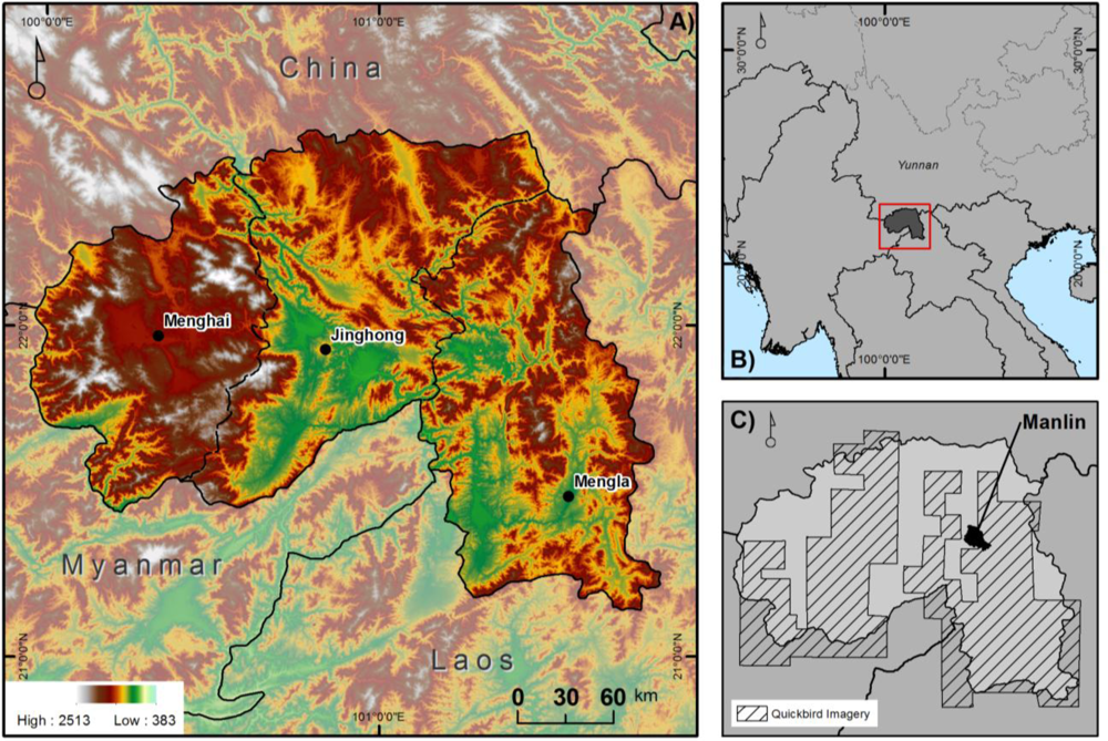
2. Study Area
3. Data and Methods
3.1. Moderate Resolution Imaging Spectroradiometer (MODIS) Data Preparation
3.2. Reference Data
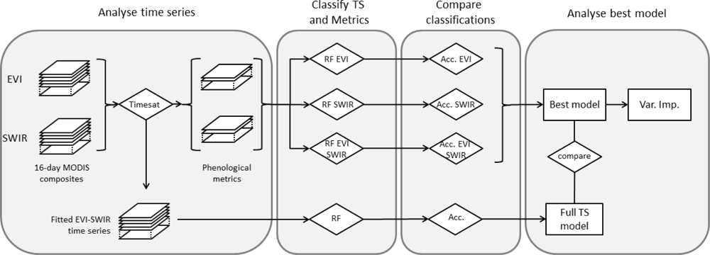
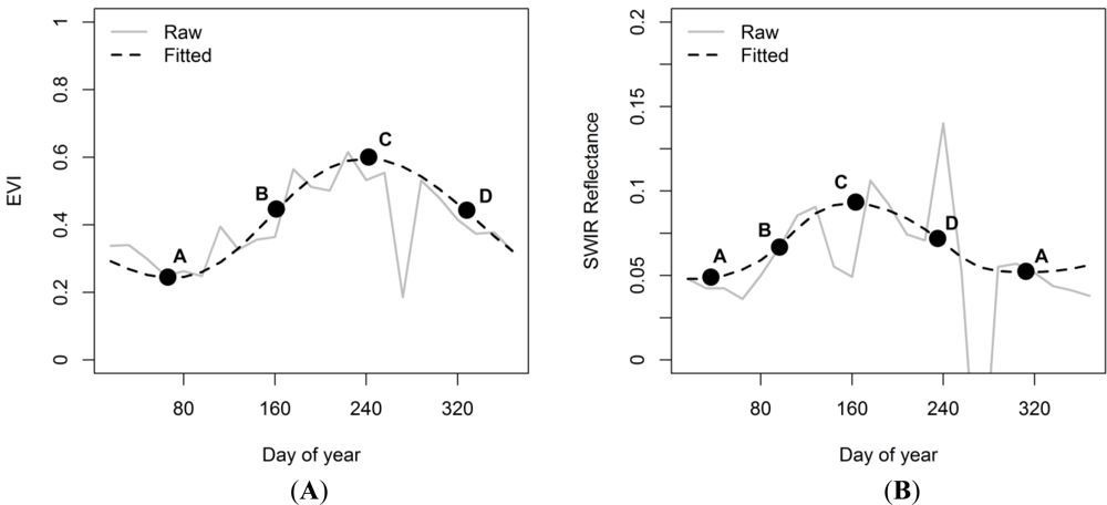
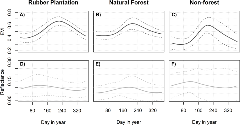
3.3. Time Series Analysis
3.4. Classification Algorithm, Variable Importance, and Accuracy Assessment
4. Results
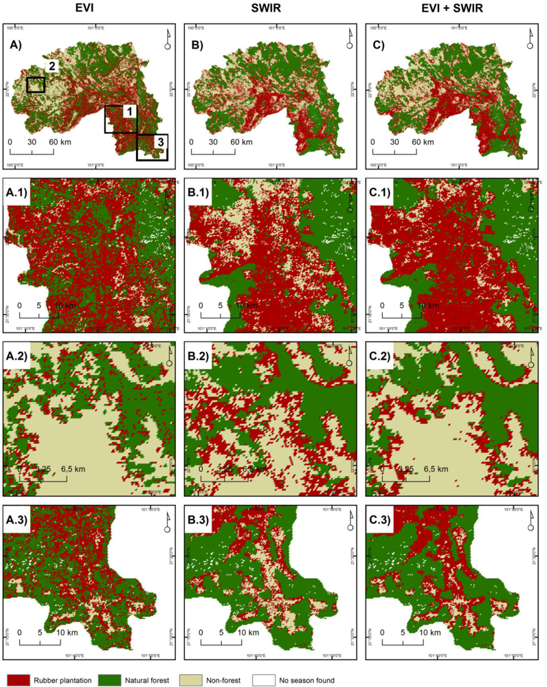
4.1. Classification Results
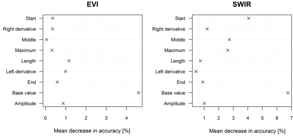
4.2. Variable Importance
5. Discussion
6. Conclusion
Acknowledgments
- Conflict of InterestThe authors declare no conflict of interest.
References
- Turner, B.L., II; Lambin, E.F.; Reenberg, A. The emergence of land change science for global environmental change and sustainability. Proc. Nat. Acad. Sci. USA 2007, 104, 20666–20671. [Google Scholar]
- Friedl, M.A.; McIver, D.K.; Hodges, J.C.F.; Zhang, X.Y.; Muchoney, D.; Strahler, A.H.; Woodcock, C.E.; Gopal, S.; Schneider, A.; Cooper, A.; et al. Global land cover mapping from MODIS: algorithms and early results. Remote Sens. Environ. 2002, 83, 287–302. [Google Scholar]
- Hansen, M.C.; DeFries, R.S.; Townshend, J.R.G.; Carroll, M.; Dimiceli, C.; Sohlberg, R.A. Global percent tree cover at a spatial resolution of 500 meters: First results of the MODIS vegetation continuous fields algorithm. Earth Interact. 2003, 7, 1–15. [Google Scholar]
- Pittman, K.; Hansen, M.C.; Becker-Reshef, I.; Potapov, P.V.; Justice, C.O. Estimating global cropland extent with multi-year MODIS data. Remote Sens. 2010, 2, 1844–1863. [Google Scholar]
- Ziegler, A.D.; Fox, J.M.; Xu, J. Agriculture. The rubber juggernaut. Science 2009, 324, 1024–1025. [Google Scholar]
- Qiu, J. Where the rubber meets the garden. Nature 2009, 457, 246–247. [Google Scholar]
- Fu, Y.; Chen, J.; Guo, H.; Hu, H.; Chen, A.; Cui, J. Agrobiodiversity loss and livelihood vulnerability as a consequence of converting from subsistence farming systems to commercial plantation-dominated systems in Xishuangbanna, Yunnan, China: A household level analysis. Land Degrad. Dev. 2010, 21, 274–284. [Google Scholar]
- Sturgeon, J.C. Governing minorities and development in Xishuangbanna, China: Akha and Dai rubber farmers as entrepreneurs. Geoforum 2010, 41, 318–328. [Google Scholar]
- Li, Z.; Fox, J.M. Integrating Mahalanobis typicalities with a neural network for rubber distribution mapping. Int. J. Remote Sens. Lett. 2011, 2, 157–166. [Google Scholar]
- Hu, H.; Liu, W.; Cao, M. Impact of land use and land cover changes on ecosystem services in Menglun, Xishuangbanna, Southwest China. Environ. Monit. Assess. 2008, 146, 147–156. [Google Scholar]
- Li, H.M.; Aide, T.M.; Ma, Y.X.; Liu, W.J.; Cao, M. Demand for rubber is causing the loss of high diversity rain forest in SW China. Biodivers. Conserv. 2007, 16, 1731–1745. [Google Scholar]
- Alcantara, P.C.; Radeloff, V.C.; Prishchepov, A.; Kuemmerle, T. Mapping abandoned agriculture with multi-temporal MODIS satellite data. Remote Sens. Environ. 2012, 124, 334–347. [Google Scholar]
- Sun, H.S.; Xu, A.G.; Lin, H.; Zhang, L.P.; Mei, Y. Winter wheat mapping using temporal signatures of MODIS vegetation index data. Int. J. Remote Sens. 2012, 33, 5026–5042. [Google Scholar]
- Hüttich, C.; Herold, M.; Wegmann, M.; Cord, A.; Strohbach, B.; Schmullius, C.; Dech, S. Assessing effects of temporal compositing and varying observation periods for large-area land-cover mapping in semi-arid ecosystems: Implications for global monitoring. Remote Sens. Environ. 2011, 115, 2445–2459. [Google Scholar]
- Hüttich, C.; Gessner, U.; Herold, M.; Strohbach, B.J.; Schmidt, M.; Keil, M.; Dech, S. On the suitability of MODIS time series metrics to map vegetation types in dry savanna ecosystems: A case study in the Kalahari of NE Namibia. Remote Sens. 2009, 1, 620–643. [Google Scholar]
- Clark, M.L.; Aide, T.M.; Grau, H.R.; Riner, G. A scalable approach to mapping annual land cover at 250 m using MODIS time series data: A case study in the Dry Chaco ecoregion of South America. Remote Sens. Environ. 2010, 114, 2816–2832. [Google Scholar]
- Tuanmu, M.N.; Vina, A.; Bearer, S.; Xu, W.H.; Ouyang, Z.Y.; Zhang, H.M.; Liu, J.G. Mapping understory vegetation using phenological characteristics derived from remotely sensed data. Remote Sens. Environ. 2010, 114, 1833–1844. [Google Scholar]
- Tottrup, C.; Rasmussen, M.S.; Eklundh, L.; Jonsson, P. Mapping fractional forest cover across the highlands of mainland Southeast Asia using MODIS data and regression tree modelling. Int. J. Remote Sens. 2007, 28, 23–46. [Google Scholar]
- Li, Z.; Fox, J.M. Mapping rubber tree growth in mainland Southeast Asia using time-series MODIS 250 m NDVI and statistical data. Appl. Geogr. 2012, 32, 420–432. [Google Scholar]
- Dong, J.; Xiao, X.; Sheldon, S.; Biradar, C.; Xie, G. Mapping tropical forests and rubber plantations in complex landscapes by integrating PALSAR and MODIS imagery. ISPRS J. Photogramm. 2012, 74, 20–33. [Google Scholar]
- Xiao, X.; Boles, S.; Frolking, S.; Li, C.; Babu, J.Y.; Salas, W.; Moore, B. Mapping paddy rice agriculture in South and Southeast Asia using multi-temporal MODIS images. Remote Sens. Environ. 2006, 100, 95–113. [Google Scholar]
- Xiao, X.; Boles, S.; Liu, J.; Zhuang, D.; Frolking, S.; Li, C.; Salas, W.; Moore, B. Mapping paddy rice agriculture in southern China using multi-temporal MODIS images. Remote Sens. Environ. 2005, 95, 480–492. [Google Scholar]
- Xiao, X.M.; Boles, S.; Liu, J.Y.; Zhuang, D.F.; Liu, M.L. Characterization of forest types in Northeastern China, using multi-temporal SPOT-4 VEGETATION sensor data. Remote Sens. Environ. 2002, 82, 335–348. [Google Scholar]
- Delbart, N.; Kergoat, L.; Le Toan, T.; Lhermitte, J.; Picard, G. Determination of phenological dates in boreal regions using normalized difference water index. Remote Sens. Environ. 2005, 97, 26–38. [Google Scholar]
- Delbart, N.; Le Toan, T.; Kergoat, L.; Fedotova, V. Remote sensing of spring phenology in boreal regions: A free of snow-effect method using NOAA-AVHRR and SPOT-VGT data (1982–2004). Remote Sens. Environ. 2006, 101, 52–62. [Google Scholar]
- Cohen, W.B.; Goward, S.N. Landsat’s role in ecological applications of remote sensing. Bioscience 2004, 54, 535–545. [Google Scholar]
- Dong, J.; Xiao, X.; Chen, B.; Torbick, N.; Jin, C.; Zhang, G.; Biradar, C. Mapping deciduous rubber plantations through integration of PALSAR and multi-temporal Landsat imagery. Remote Sens. Environ. 2013, 134, 392–402. [Google Scholar]
- Pu, Y.-S.; Zhang, Z.-Y. A strategic study on biodiversity coservation in Xishuangbanna. J. Forestry Res. 2001, 12, 25–30. [Google Scholar]
- Chapman, E.C. The expansion of rubber in southern Yunnan, China. Geogr. J. 1991, 157, 36–44. [Google Scholar]
- Guardiola-Claramonte, M.; Troch, P.A.; Ziegler, A.D.; Giambelluca, T.W.; Durcik, M.; Vogler, J.B.; Nullet, M.A. Hydrologic effects of the expansion of rubber (Hevea brasiliensis) in a tropical catchment. Ecohydrology 2010, 3, 306–314. [Google Scholar]
- Zhu, H.; Cao, M.; Hu, H. Geological history, flora, and vegetation of Xishuangbanna, Southern Yunnan, China. Biotropica 2006, 38, 310–317. [Google Scholar]
- Cao, M.; Zou, X.; Warren, M.; Zhu, H. Tropical Forests of Xishuangbanna, China. Biotropica 2006, 38, 306–309. [Google Scholar]
- Cao, S.; Wang, X.; Song, Y.; Chen, L.; Feng, Q. Impacts of the Natural Forest Conservation Program on the livelihoods of residents of Northwestern China: Perceptions of residents affected by the program. Ecol. Econ. 2010, 69, 1454–1462. [Google Scholar]
- Zhang, J.; Cao, M. Tropical forest vegetation of Xishuangbanna, SW China and its secondary changes, with special reference to some problems in local nature conservation. Biol. Conserv. 1995, 73, 229–238. [Google Scholar]
- Huete, A.; Didan, K.; Miura, T.; Rodriguez, E.P.; Gao, X.; Ferreira, L.G. Overview of the radiometric and biophysical performance of the MODIS vegetation indices. Remote Sens. Environ. 2002, 83, 195–213. [Google Scholar]
- Tortora, R.D. A note on sample size estimation for multinomial populations. Am. Stat. 1978, 32, 100–102. [Google Scholar]
- Congalton, R.G.; Green, K. Assessing the Accuracy of Remotely Sensed Data: Principales and Practices; CRC Press: Boca Raton, FL, USA, 2008; Volume 2. [Google Scholar]
- Joensson, P.; Eklundh, L. TIMESAT—A program for analyzing time-series of satellite sensor data. Comput. Geosci. 2004, 30, 833–845. [Google Scholar]
- Jonsson, P.; Eklundh, L. Seasonality extraction by function fitting to time-series of satellite sensor data. IEEE Trans. Geosci. Remote Sens. 2002, 40, 1824–1832. [Google Scholar]
- Breiman, L. Random forests. Mach. Learn. 2001, 45, 5–32. [Google Scholar]
- Rodriguez-Galiano, V.F.; Ghimire, B.; Rogan, J.; Chica-Olmo, M.; Rigol-Sanchez, J.P. An assessment of the effectiveness of a random forest classifier for land-cover classification. ISPRS J. Photogramm. 2012, 67, 93–104. [Google Scholar]
- Chan, J.C.-W.; Paelinckx, D. Evaluation of Random Forest and Adaboost tree-based ensemble classification and spectral band selection for ecotope mapping using airborne hyperspectral imagery. Remote Sens. Environ. 2008, 112, 2999–3011. [Google Scholar]
- Gislason, P.; Benediktsson, J.; Sveinsson, J. Random forests for land cover classification. Pattern Recognit. Lett. 2006, 27, 294–300. [Google Scholar]
- Foody, G.M. Status of land cover classification accuracy assessment. Remote Sens. Environ. 2002, 80, 185–201. [Google Scholar]
- Archer, K.J.; Kimes, R.V. Empirical characterization of random forest variable importance measures. Comput. Stat. Data An. 2008, 52, 2249–2260. [Google Scholar]
- R Development Core Team. R: A Language and Environment for Statistical Computing; R Foundation for Statistical Computing: Vienna, Austria, 2011. [Google Scholar]
- Liaw, A.; Wiener, M. Classification and regression by randomForest. R News 2002, 2/3, 18–22. [Google Scholar]
- Chen, C.; Liaw, A.; Breiman, L. Using Random Forest to Learn Imbalanced Data; University California-Berkley: Berkeley, CA, USA, 2004. [Google Scholar]
- Tuanmu, M.N.; Vina, A.; Roloff, G.J.; Liu, W.; Ouyang, Z.Y.; Zhang, H.M.; Liu, J.G. Temporal transferability of wildlife habitat models: Implications for habitat monitoring. J. Biogeog. 2011, 38, 1510–1523. [Google Scholar]
- Wang, L.; Qu, J.J.; Hao, X.; Zhu, Q. Sensitivity studies of the moisture effects on MODIS SWIR reflectance and vegetation water indices. Int. J. Remote Sens. 2008, 29, 7065–7075. [Google Scholar]


| Class | Description | Number of Pixels |
|---|---|---|
| Rubber plantation | Areas covered by rubber trees in varying stand density. Undergrowth varies between open soil and fruits. | 154 (30%) |
| Forest | Primary and secondary forests with a canopy cover greater than 40%. | 257 (49%) |
| Non-forest | Areas not covered by rubber plantations or natural forests. Mostly covered by crops (eggplant, rice, corn, pineapple, melon, among others), as well as areas with artificial land cover (urban and transportation), water, and shrubs. | 109 (21%) |
| Land Cover | Accuracy (%) | |||||
|---|---|---|---|---|---|---|
| EVI | SWIR | EVI and SWIR | ||||
| Producer’s | User’s | Producer’s | User’s | Producer’s | User’s | |
| Rubber plantation | 55.2 | 50.6 | 61.0 | 61.8 | 63.6 | 64.9 |
| Forest | 66.5 | 78.4 | 80.2 | 79.2 | 80.2 | 84.8 |
| Non-forest | 72.5 | 59.0 | 48.6 | 49.1 | 71.6 | 61.9 |
| Overall | 64.4 | 67.9 | 73.5 | |||
| Reference | Classification | |||
|---|---|---|---|---|
| Rubber | Forest | Non-Forest | Producer’s Accuracy | |
| Rubber | 98 | 25 | 31 | 63.6% |
| Forest | 34 | 206 | 17 | 80.2% |
| Non-forest | 19 | 12 | 78 | 71.6% |
| User’s accuracy | 64.9% | 84.8% | 61.9% | |
© 2013 by the authors; licensee MDPI, Basel, Switzerland This article is an open access article distributed under the terms and conditions of the Creative Commons Attribution license (http://creativecommons.org/licenses/by/3.0/).
Share and Cite
Senf, C.; Pflugmacher, D.; Van der Linden, S.; Hostert, P. Mapping Rubber Plantations and Natural Forests in Xishuangbanna (Southwest China) Using Multi-Spectral Phenological Metrics from MODIS Time Series. Remote Sens. 2013, 5, 2795-2812. https://doi.org/10.3390/rs5062795
Senf C, Pflugmacher D, Van der Linden S, Hostert P. Mapping Rubber Plantations and Natural Forests in Xishuangbanna (Southwest China) Using Multi-Spectral Phenological Metrics from MODIS Time Series. Remote Sensing. 2013; 5(6):2795-2812. https://doi.org/10.3390/rs5062795
Chicago/Turabian StyleSenf, Cornelius, Dirk Pflugmacher, Sebastian Van der Linden, and Patrick Hostert. 2013. "Mapping Rubber Plantations and Natural Forests in Xishuangbanna (Southwest China) Using Multi-Spectral Phenological Metrics from MODIS Time Series" Remote Sensing 5, no. 6: 2795-2812. https://doi.org/10.3390/rs5062795