Abstract
Vegetation in the Arctic is often sparse, spatially heterogeneous, and difficult to model. Synthetic Aperture Radar (SAR) has shown some promise in above-ground phytomass estimation at sub-arctic latitudes, but the utility of this type of data is not known in the context of the unique environments of the Canadian High Arctic. In this paper, Artificial Neural Networks (ANNs) were created to model the relationship between variables derived from high resolution multi-incidence angle RADARSAT-2 SAR data and optically-derived (GeoEye-1) Soil Adjusted Vegetation Index (SAVI) values. The modeled SAVI values (i.e., from SAR variables) were then used to create maps of above-ground phytomass across the study area. SAVI model results for individual ecological classes of polar semi-desert, mesic heath, wet sedge, and felsenmeer were reasonable, with r2 values of 0.43, 0.43, 0.30, and 0.59, respectively. When the outputs of these models were combined to analyze the relationship between the model output and SAVI as a group, the r2 value was 0.60, with an 8% normalized root mean square error (% of the total range of phytomass values), a positive indicator of a relationship. The above-ground phytomass model also resulted in a very strong relationship (r2 = 0.87) between SAR-modeled and field-measured phytomass. A positive relationship was also found between optically derived SAVI values and field measured phytomass (r2 = 0.79). These relationships demonstrate the utility of SAR data, compared to using optical data alone, for modeling above-ground phytomass in a high arctic environment possessing relatively low levels of vegetation.
1. Introduction
Knowledge of the spatial distribution of vegetation cover and phytomass in the High Arctic is becoming increasingly important due to the changing climate of this region. Vegetation is very limited in arctic environments, especially in the High Arctic bioclimatic zones [1,2]. The limited vegetation that is present, however, can have significant effects on the terrestrial carbon balance [3,4] and methane fluxes [5]. Further, knowledge of vegetation density is important for monitoring forage quality and quantity for ungulates such as Peary Caribou (listed as Endangered in the Canadian Species At Risk Act) and muskoxen [6,7].
In addition to the obvious limitations of air and soil temperature, there are a number of factors that serve as controls on vegetation growth in the high arctic, including soil moisture [8,9], available nutrients [10,11], topography [12,13], microtopography [8,12,14], and soil type [14]. The variation and distribution of these different environmental controls results in a very heterogeneous vegetation cover, with very different vegetation ecosystems sometimes in close proximity to one other. Remote sensing is therefore the best tool available to accurately map the spatial distribution of above-ground phytomass at the fine scales necessary to distinguish between these vegetation community types. This fine-scale mapping is crucial for accurate carbon budgets and phytomass estimation at the local scale [15], and also for accurately scaling up these variables to larger regional scales [16,17]. Vegetation cover can also complicate the retrieval of other important biophysical parameters, such as soil moisture, when using Synthetic Aperture Radar (SAR) [18,19]; however, if vegetation cover is known, soil moisture retrieval accuracy can be increased [19,20].
SAR has been used in vegetation/biomass studies at sub-arctic latitudes [21,22], but is very rarely used to study arctic vegetation [23], and has not been used at all in the context of the High Arctic. There are considerable benefits to using SAR when compared to optical data for arctic research. Acquiring cloud-free optical images is often problematic in the arctic, and low solar zenith angles at high latitudes can also cause illumination issues with optical data [19]. There are also challenges with using SAR to model vegetation in the High Arctic, however, such as the extremely limited amounts of phytomass in all but the wettest areas. Even so, there are a number of approaches to modeling backscatter from vegetation canopies (see review in [19] and [24]). These approaches, however, only apply when the vegetation is dense enough to form some sort of canopy, i.e., the above-ground phytomass must be of a sufficient height to have a noticeable effect on backscatter, which may not hold true in many parts of the arctic. Agricultural studies have demonstrated that even relatively short vegetation can produce an appreciable amount of HV backscatter due to depolarization [21,25] of the backscatter, as well as marked differences in HH and VV polarizations [22], though high arctic vegetation levels are generally even lower than short-crop agriculture. Low density grasses and sedges, which make up much of the vegetation cover in the high arctic, can also be difficult to distinguish from bare ground [26]. Regardless, polarimetric data could be key to this analysis if this depolarization holds true for very low levels of vegetation. Multiple incidence angle data may be important for similar reasons, with greater incidence angle backscatter having greater interaction (and therefore backscatter) with short vegetation than smaller incidence angle data [21,22,27] (similar to how surface roughness affects backscatter), though stopping short of full volumetric scatter.
The Radar Vegetation Index (RVI), which has been used to estimate biomass from SAR data [20,28] characterizes vegetation scattering by dividing the cross-polarization scattering by the total scattering; effectively measuring the degree of depolarization. RVI may not be applicable if there is little to no volume scattering present, as would be the case below a certain threshold level of vegetation indicated by a lower HV backscatter contribution. If the vegetation cover is sparse or very dry, the surface roughness may be the most significant contributor to total backscatter [29,30].
Vegetation can be modeled using not only relations of SAR to above-ground phytomass (as described above), but also using other controlling factors as input. As mentioned previously, vegetation in the high arctic is closely related to topographic and moisture gradients across the landscape, so variables derived from a Digital Elevation Model (DEM) have the potential to be useful for vegetation modeling. Vegetation biomass can be a good proxy for soil moisture in the arctic, due to the vegetation being dependent on the spatial distribution of soil moisture (i.e., it only grows in areas with consistently high soil moisture, with drier areas being completely barren) [31]. Once vegetation is modeled, it can therefore be used to help model soil moisture using SAR over the same areas [19,32], or vice versa. The inclusion of multiple data types from different sources into the model suggests that the use of Artificial Neural Networks (ANNs) would be a practical way to model the vegetation.
ANNs are commonly used to invert surface parameters from SAR data [33,34], and show great promise in both simplifying the modeling process and increasing the accuracy of the results. ANNs have the capacity to “learn” complex, nonlinear patterns, and generalize these patterns in noisy environments. This capacity to generalize means that ANNs can be effective in situ ations where data may be missing or imprecise. ANNs are also able to incorporate prior knowledge and physical constraints into the analysis, while making no assumptions about the statistical nature of the input data [35,36]. This allows for the incorporation of disparate data from many remote sensing and ancillary sources, and can include variables such as terrain height, slope, aspect, soil texture and land cover. ANNs are superior at generalizing (or extending) results for application to new areas than a strictly empirical model, and do not have the same parameterization problems and assumption difficulties as physical models. The target variable for the ANN model needs to be a spatially explicit measure of vegetation phytomass, so a vegetation index from high resolution multi-spectral data is ideal.
Raynolds et al. [37] established that maximum annual Normalized Difference Vegetation Index (NDVI) values from coarse spatial resolution imagery are closely related to peak summer above-ground phytomass across a range of sites in the arctic along a latitudinal gradient. Previous research at the Cape Bounty study location used in this analysis, using high spatial resolution imagery to generate NDVI, demonstrates a weaker relationship [9], possibly due to the differences in the range of phytomass levels sampled (i.e., Raynolds sampled across five bioclimatic zones), spatial resolutions, or vegetation characteristics unique to Cape Bounty. Other vegetation variables were more closely correlated to high spatial resolution NDVI, such as Percent Vegetation Cover (PVC) [9], vegetation volume [38], and Leaf Area Index [4]. A large proportion of the phytomass is made up of bryophytes in the high arctic [37,39], with Cape Bounty being no exception, and this is thought to be a confounding factor in the relationships of NDVI to these other vegetation variables, due to the differing NDVI reflectance characteristics of bryophytes and vascular plants [40–42]. It is not clear as to the effects of bryophytes on SAR backscatter in this environment, although their ability to absorb and retain moisture likely influences the dielectric properties at the surface. Watanabe et al. [43], in a study using L-band SAR, discovered that moss layers in permafrost environments have a significant impact on co-pol backscattering (though not cross-pol backscatter), so the effects on C-band SAR, as used in this study, are likely to be noticeable, especially if the bryophytes are holding water.
Previous studies in the High Arctic have noted the fine-scale topographic and moisture controls of the ice-wedge polygon and frost crack dominated landscape [8,14]. Vegetation in polar semi-desert areas is often limited to the margins of the polygons, where wind speed is reduced and sufficient moisture and nutrients are present to allow growth; these features therefore leave large patches of bare ground. This high proportion of bare ground can dominate the NDVI signal, causing an underestimation of above-ground phytomass for the area. Previous research has suggested that using the Soil Adjusted Vegetation Index (SAVI) [44], which takes into account larger proportions of bare ground in the signal, could ameliorate the NDVI underestimation of above-ground phytomass [8,45]. Optical data will therefore be used to generate SAVI values across the study area to be used as a baseline for the vegetation modeling.
The purposes of this research are two-fold: (i) to determine the effects that high arctic vegetation has on SAR backscatter, including polarimetric effects; and (ii) to model vegetation phytomass using an Artificial Neural Network (ANN). The results of the ANN will then be related to above-ground phytomass levels. Due to the low levels of vegetation phytomass in the study area, it is not expected that the vegetation itself will have strong interactions with the SAR signals, but it is likely that changes in soil moisture and surface roughness that would be strongly associated with areas of higher phytomass could be detected more easily.
2. Methods
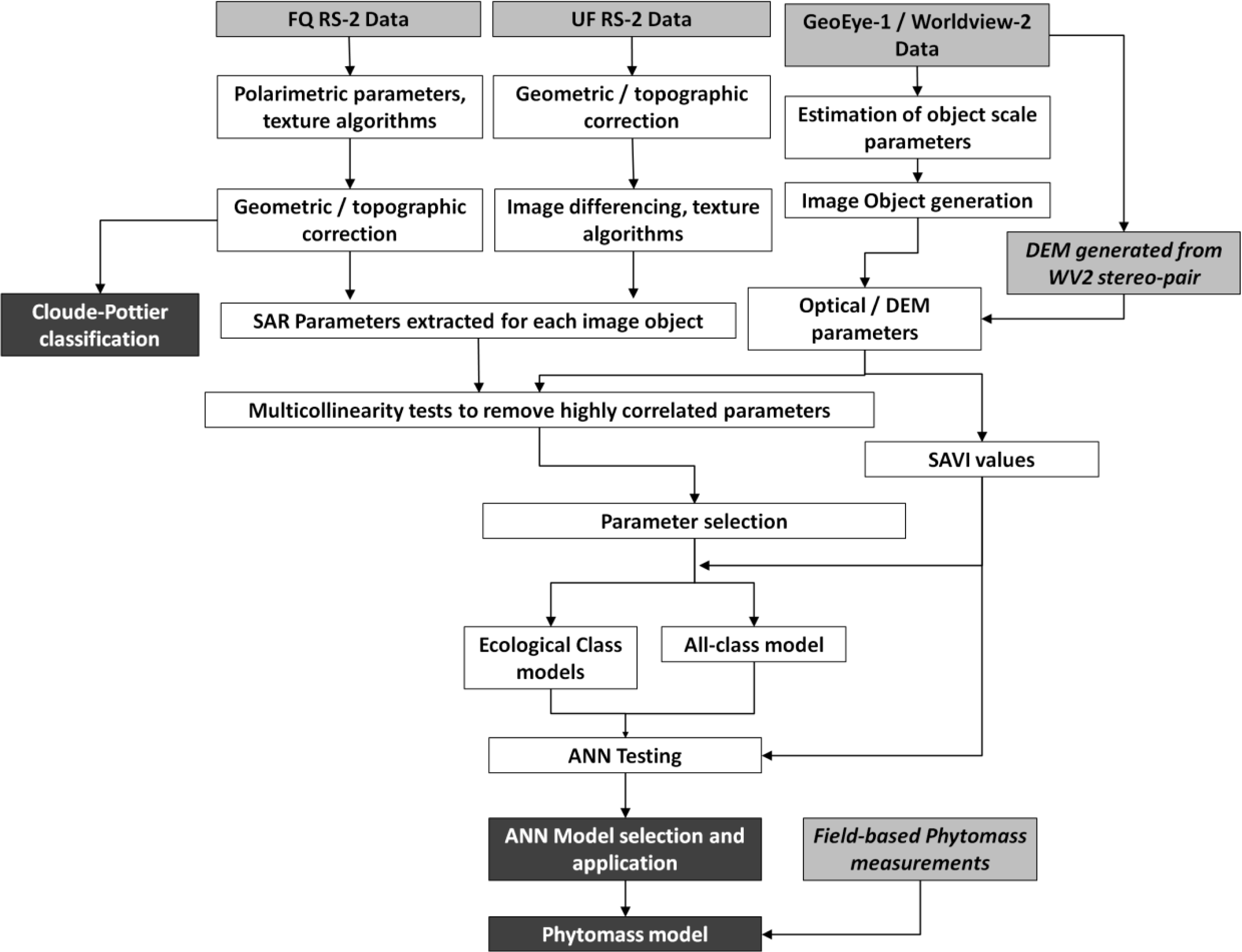
Before creating the ANN models, the study area was segmented into discrete image objects using the multi-spectral data. Once this was completed, the variables to be used as the model input were determined. A variety of difference variables, texture variables, and, in the case of the polarimetric data, polarimetric variables and decompositions, were derived and extracted from the SAR data. These variables were averaged within the image objects, and then analyzed for multicollinearity and correlation to multi-spectral derived SAVI values. The models were then applied to larger scale image objects, and also used to model above-ground phytomass (Figure 1).

Figure 1.
Methodology diagram showing data sources (light grey) and outputs (dark grey). FQ and UF inputs are Fine-Quad polarimetric and UF inputs are Ultra-fine single polarization (HH) RADARSAT-2 data.
2.1. Study Location and Site Description
Field work for this study was conducted at the Cape Bounty Arctic Watershed Observatory (CBAWO), located on southern Melville Island in Nunavut, Canada (approximately 74.91°N, 109.44°W) in 2009 and 2010 (Figure 2). The CBAWO is composed of two parallel watersheds that, when combined, cover approximately 15 km2. The topography is rolling, with low to medium relief; elevation ranges from 5 m to 125 m above sea level. Past glaciation has deposited various tills in the region, primarily Winter Harbour till [46], which is a thin (1–2 m) carbonate rich till that is draped over the other layers [46]. There are also Holocene-era clay-rich marine sediments, which are located between about 35 m and 90 m above sea level [46,47]. According to the Circumpolar Arctic Vegetation Map [48], Cape Bounty is located in bioclimatic zone B, with a vegetation classification of G2-graminoid, prostrate dwarf shrub, forb tundra.
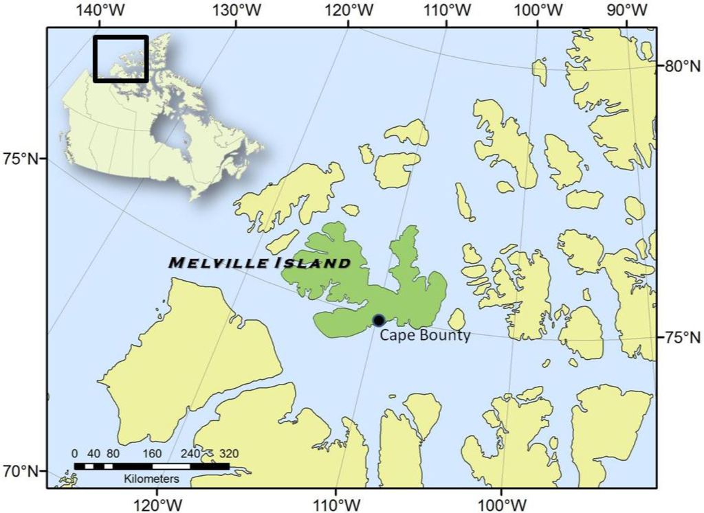
Figure 2.
Study location on Melville Island, Nunavut, Canada.
Vegetation in the area is extremely heterogeneous, and consists of bryophytes, forbs, graminoids, and prostrate shrub species (i.e., Salix arctica). The vegetation can be classified into three main ecological types based on topographic and moisture conditions: polar semi-desert, mesic tundra, and wet sedge tundra. Greater phytomass is found in the mesic and sedge communities, which have large amounts of bryophytes and graminoids. Mesic areas are more sparsely vegetated than the sedge areas, but can have equal or greater phytomass due to large quantities of bryophytes [45]. Polar semi-desert areas can be completely barren, but are often characterized by patterned ground features with vegetation cover found in depressions. In areas that do contain vegetation, phytomass values range from about 200 to 2200 g/m2. Phytomass values in the lower end of this range are not expected to be detectable by SAR. Large areas of exposed, fractured bedrock are also present, and the entire area is underlain by permafrost, with an active layer of 0.5 m–1 m during the summer.
2.2. Optical Imagery
A high spatial resolution (1 m) Digital Elevation Model (DEM) was derived from a Worldview-2 stereopair (15 July 2012) at Cape Bounty and used for orthorectification of the optical and SAR data, as well as for generating the Topographic Position Index (TPI) variable. The TPI is a method of defining the relative position of a given location along a topographic gradient [49], where negative values represent valley or slope bottoms, values near zero represent flat areas or midslope areas, and positive values represent ridge tops and hills. The TPI was calculated using a 150 m radius window on the 1 m spatial resolution DEM [50].
2.3. Object-Based Image Analysis (OBIA)
High resolution multispectral data (i.e., GeoEye-1) collected at Cape Bounty (22 August 2009), were pan-sharpened to 0.5 m spatial resolution, and orthorectified using ground control points in the form of corner reflectors (set up for the SAR imagery, but were identifiable in the optical imagery as well). The image was then atmospherically corrected using the ATCOR algorithm as implemented in PCI Geomatica 2013. In the absence of comprehensive field data, SAVI data were generated to validate the ANN models; these data provide a spatially comprehensive surrogate for field measures of vegetation. The correction value, L, was set to 0.5 for the SAVI calculation (Equation (1)), where NIR is the Near-infrared band, and RED is the visible red band.
The vegetation model was constructed using OBIA, in which image objects consisting of groups of spectrally similar pixels are used as the minimum mapping unit, rather than individual pixels. OBIA has a number of advantages over pixel-based methods, including reduced dependency on noise-filtering algorithms (especially with SAR data), and the ability to investigate different spatial scales by simply changing the size of the image objects. OBIA is recognized as a very effective tool for analyzing geo-spatial and remotely-sensed data [51]. Image objects were generated from the 0.5 m pan-sharpened GeoEye-1 imagery (described above) for the CBAWO using eCognition® 8.64 software. Near-infrared, red, and green bands were used for grouping spectrally similar pixels, in order for the objects to be representative of the vegetation ecology on the ground. Two image object sizes that were physically meaningful [52,53] were chosen, with the smaller objects for both locations ranging between approximately 50 and 6000 m2, and the larger objects ranging from 50 to 35,000 m2 in size.
2.4. SAR Data
RADARSAT-2 data were used to take advantage of the relatively high resolution beam modes and fully polarimetric data. SAR data were collected at various incidence angles over the study area during the summers of 2009 and 2010 (Table 1) with both the Ultra-Fine (U) and Fine-Quad (FQ) beam modes. The Ultra-Fine beam mode has a spatial resolution of 3 m, though it is limited to a single polarization. The Fine-Quad products are fully polarimetric, but have a slightly coarser spatial resolution, at 8 m. Although additional SAR scenes were collected, those presented in Table 1 were identified as being relatively snow-free and uncompromised by active precipitation.

Table 1.
RADARSAT-2 data used in the analysis.
Ultra-Fine mode data were orthorectified before further analysis, while the Fine-Quad data were analyzed in slant range to preserve polarimetric information, and were only orthorectified to extract the plot data for each variable after the variables were calculated for the scene. Nine corner reflectors spaced around the watersheds of Cape Bounty were used to assist with geometric correction. Speckle filtering was not performed explicitly, except for the calculation of the RVI and the Cloude-Pottier decomposition [54]; it was otherwise handled through image-object averaging (discussed below).
2.5. Vegetation Modeling
Polarimetric decompositions were analyzed to determine the nature of the SAR backscatter in this low vegetation terrain. Comparing the Cloude-Pottier decomposition values of entropy and alpha angle (H-α) between bare and vegetated surfaces could give an indication of the strength of the effect that vegetation has on backscatter, as these parameters change based on the type of scattering mechanism present on the surface [54]. Other SAR-derived parameters, such as the RVI, were also examined in this context. The low levels of phytomass in this environment (<2200 g/m2), are not expected to produce noticeable dipole or volumetric scatter, and this analysis of the scattering mechanisms present is included to confirm this suspicion. For similar reasons, HV backscatter is not expected to change significantly between areas of high and low phytomass. The physical structure of the vegetation present in this area, mainly grass/sedge and small forbs, also does not, in theory, lend itself to useable levels of VV backscatter. HH backscatter is expected to be more variable with changing amounts of phytomass.
The SAR-derived parameters evaluated for inclusion to the ANN models are given in Table 2. The texture variables [55,56] were calculated on a per-pixel basis using an 11 × 11 pixel window for each RADARSAT-2 scene, before being averaged for each image object. Other variables are simple means of the pixel values for each image object. The texture measures for the U and FQ scenes were calculated using the HH backscatter intensity. The natural logarithm of the Normalized Backscatter Roughness Index (Ln(NBRI)) [57] variable was computed using the U75 and U26 scenes (Table 1) to maximize the incidence angle difference.

Table 2.
Variables generated from Synthetic Aperture Radar (SAR) data. Variables in italics are additional variables applicable only to the fully polarimetric FQ data.
In addition to the SAR-derived variables, the TPI variable was also included in the analysis. Variables that were not directly correlated (Pearson |r| < ∼0.3) with the optical-derived SAVI values for each image object were removed from further analysis. Visual analysis of scatter plots helped to reveal possible non-linear correlations that the Pearson correlation would not identify. Variables that were highly correlated (Spearman |ρ| > ∼0.8) with other remaining variables were also removed to alleviate concerns over multicollinearity, which can be a problem when training ANNs.
A series of ANN models were then implemented to model the relationships between the remaining variables and the SAVI values. The neural network implementation of the MATLAB® software package was used in the development of the ANN; it is a two-layer feed-forward network with sigmoid-function hidden neurons and linear-function output neurons, trained with the Levenberg-Marquardt backpropagation algorithm [58]. One ANN was developed using all of the image objects from Cape Bounty together, and others were developed using separate models for each ecological class as defined and mapped for the area by Atkinson and Treitz [45]. These four ecological classes are derived based on a vegetation and moisture gradient, and are characteristic of the local vegetation ecology. The ecological classes (eco-classes) are polar semi-desert, mesic tundra, wet sedge, and felsenmeer/rock. The polar semi-desert and felsenmeer/rock classes have the lowest above-ground phytomass values, with mesic tundra and wet sedge having higher values.
A number of image objects were excluded from the analysis, both from the initial model development with the smaller image objects, and for the model application with the larger image objects. Objects excluded included any classified as water or unclassified by the ecological classification [45], as well as any objects outside a 10 degree range of local incidence angle (centered on the scene-average local incidence angle for any given beam mode). This was to prevent outliers due to the effects of steep slopes and cliffs on SAR backscatter. The remaining smaller size image objects (n = 10,041) covering the Cape Bounty study area were randomly partitioned into three sets for the ANN development: 70% of the data were used for training, 15% for validation, and 15% was held back as a completely independent test set. Validation data are used as a guide on the accuracy and generalization capability of the model when fitting it to the training data. The resulting ANN models were then applied to the larger image objects (n = 1333) to determine the ability of the models to adapt to different spatial scales.
While modeling SAVI from SAR data is a good first step, it is also important to determine what those values mean on the ground in terms of above-ground phytomass in this environment. Previous attempts at relating an optical vegetation index (NDVI) to above-ground phytomass for this environment were mixed [9], with r2 values for Cape Bounty of 0.55. Other studies have found stronger relationships [3,37,59], but were at much coarser spatial resolutions. To show that the ANN results (estimated SAVI values from SAR variables) can be used to predict actual ground-based measures of above-ground phytomass, regression analyses were used with field-sampled values of above-ground phytomass collected for previous research [9]. This ANN-phytomass relationship can then be used to construct maps of above-ground phytomass levels across the study area.
3. Results and Discussion
3.1. Scattering Mechanisms
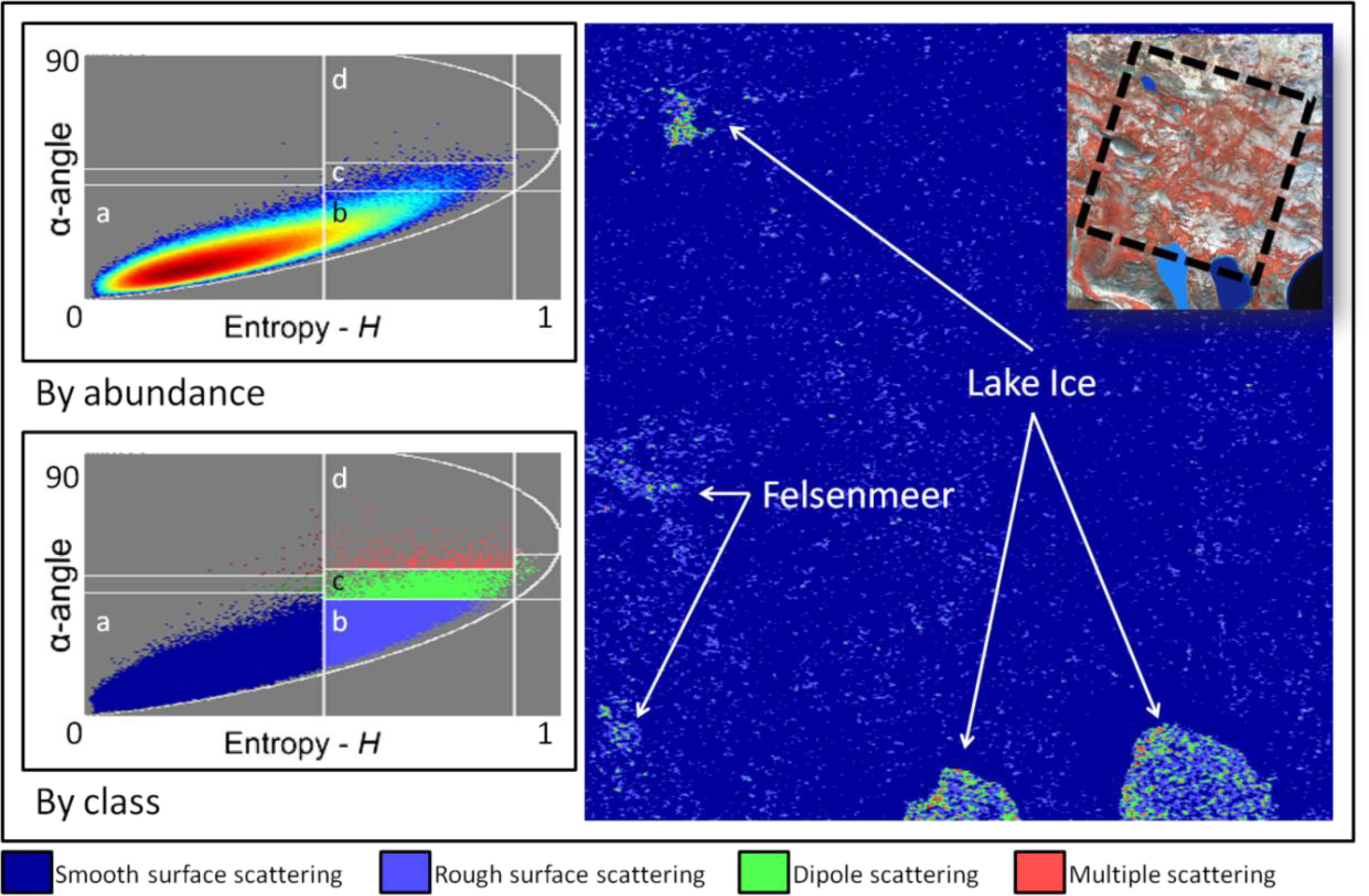
Two Fine-Quad RADARSAT-2 scenes from 8 and 23 July 2010 (Table 1) were chosen for the Cloude-Pottier analysis. The July 8 scene was a ‘wet’ scene, taken shortly after a precipitation event when the surface and the vegetation still held appreciable amounts of water, and the July 23 scene was a “dry” scene, where the surface and vegetation were not holding high levels of water. The results of these H-α classifications indicate that there is only low and medium entropy surface scattering in this study area, as expected, even in areas characterized by high above-ground phytomass. The only occurrences of non-surface scattering classes are caused by ice cover (ocean and lakes) and areas of large boulders and felsenmeer/rock (Figure 3). Similarly, the RVI was not correlated with either SAVI values or previously modeled above-ground phytomass [9]. These results therefore indicate that the levels of above-ground phytomass are not sufficient for polarimetric methods to be helpful in vegetation modeling for this study area with the available polarimetric scenes, a conclusion further supported by the lack of correlation between other SAR-derived polarimetric variables (Table 2) (including HV and VV polarizations) and SAVI values derived from the GeoEye-1 image data. The polarimetric data were acquired at steep incidence angles (<25°) to allow for more accurate soil moisture retrievals, so it is possible that there would be greater polarimetric sensitivity to the vegetation at shallower incidence angles.
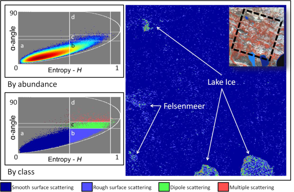
Figure 3.
Results of the Cloude-Pottier H-α decomposition and classification of FQ2 scene from 23 July 2010. (a) Low entropy (smooth) surface scattering; (b) Medium entropy (rough) surface scattering; (c) Medium entropy dipole scattering; (d) Medium entropy multiple scattering.
3.2. ANN Models
The variables that were found to correlate to SAVI, and were therefore used in the ANN, are given in Table 3. One of the disadvantages of the ANN approach is the difficulty in determining the relative contribution of each input variable to the model output, though this problem can be mitigated to some extent with careful variable selection and individual variable correlation analysis. The reasons for these correlations seem to depend on the characteristics of backscatter changes from different incidence angles, rather than any sort of textural or polarimetric information. The “Mean” values of the U2 and FQ5 scenes were correlated with SAVI, and were both included, despite being correlated to each other, due to their differences in sensitivity to different eco-types. That is, the two variables became less correlated with each other as SAVI values increased, likely due to the differences in incidence angle between the two beam modes. The Ln(NBRI) variable also seems to be correlated to SAVI due to backscatter differences from different incidence angle beam modes that are dependent on above-ground phytomass and associated soil moisture differences. Lower SAVI values correspond with higher Ln(NBRI) values. The TPI variable is also very likely sensitive to the topographic controls on the local soil moisture regime; as previously described, vegetation abundance is very closely related to moisture abundance in this environment, and topography is an important driver of moisture availability.

Table 3.
Variables derived from SAR data and elevation models used to develop the Artificial Neural Networks (ANNs).
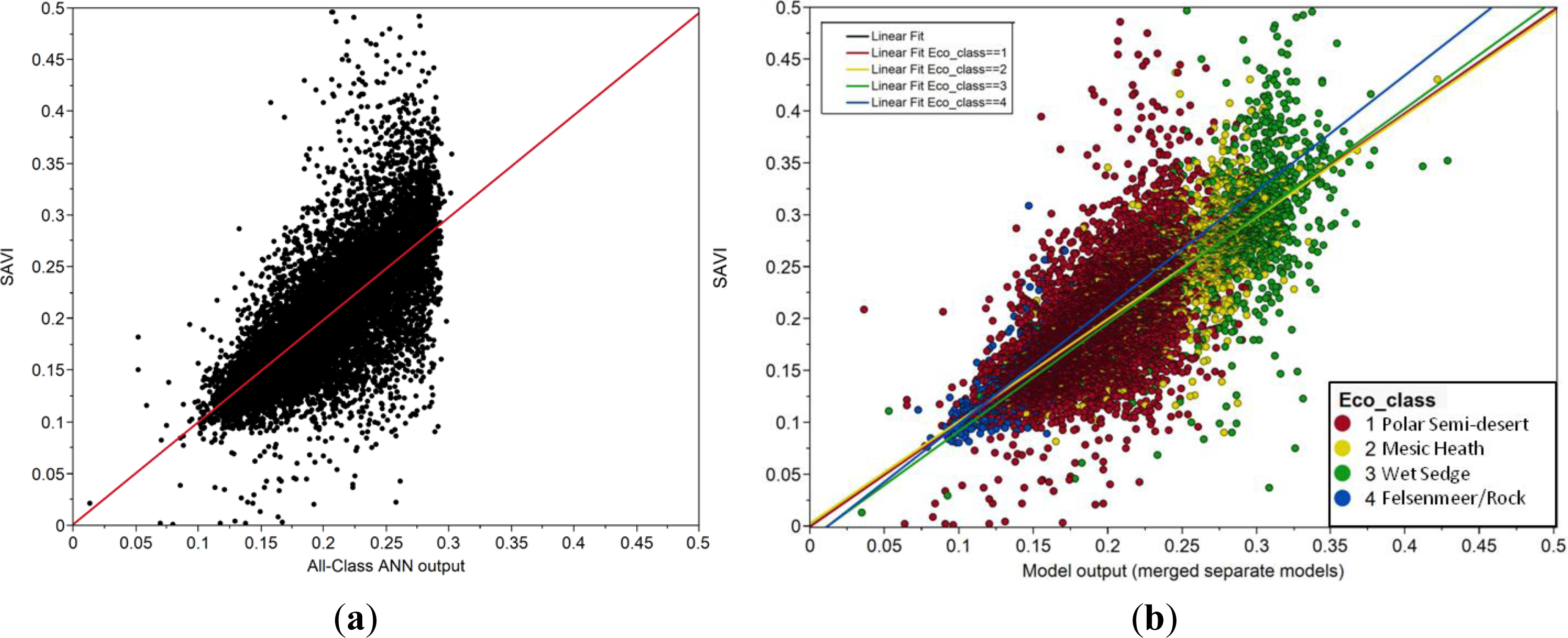
The results of the ANNs (Table 4) developed for the separate eco-classes were individually less accurate than the model generated using only a single class that included all points (all-class ANN). However, when the outputs of the separate eco-class models were merged together into one output variable to allow for a single correlation analysis to SAVI (Table 4—“combined”, Figure 4) the results are much stronger, with an r2 of 0.6, and a normalized Root Mean Square Error (N_RMSE) of 8%. The N_RMSE is the RMSE normalized to the range of SAVI values present in each dataset (% of the total range), and is a good way to directly compare the performance of the ANNs to each other. In addition, the mean values of SAVI for each image object, derived from the optical imagery, were not significantly different (p < 0.05) than the mean values of the ANN output for each image object. A closer examination of the results of the All-class ANN (Figure 4) indicates that the model loses its predictive capability beyond SAVI values of approximately 0.3. The results when separated by eco-class are much more accurate (Figures 4 and 5), even at values of SAVI above 0.3. The separate eco-class models were therefore applied to the larger image objects to determine their ability to generalize to coarser spatial resolutions.

Table 4.
ANN results for the small image objects. The “combined” results are the combination of the separate eco-class ANNs. N_RMSE is the RMSE normalized to the range of values present in the data. Mean Soil Adjusted Vegetation Index (SAVI) values are derived from the optical data for each object; mean ANN is the modeled SAVI mean for each object.
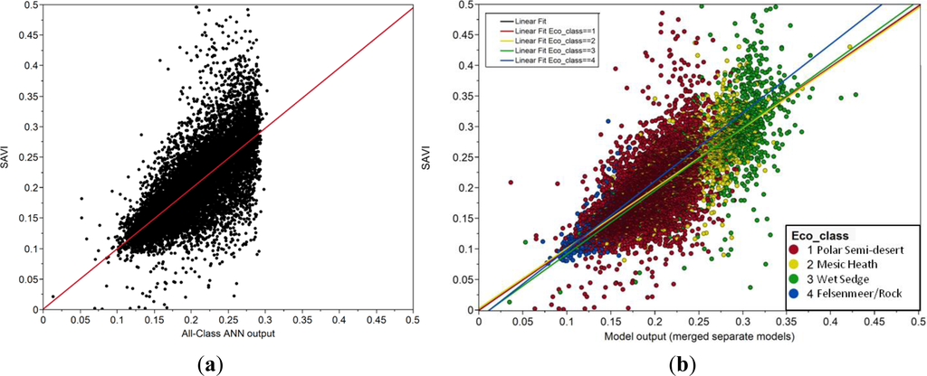
Figure 4.
(a) Output of the All-Class ANN compared to the SAVI values derived from optical data; (b) Combined ANN model output from each separate eco-class ANN, compared to SAVI values.
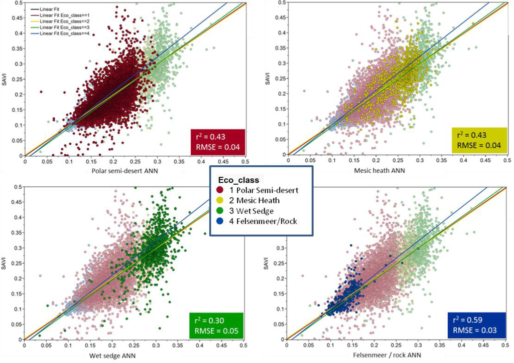
Figure 5.
Individual ANN model output from each separate eco-class ANN.
The lower r2 and higher RMSE values for the Wet Sedge eco-class could be due to factors that are influencing either the optical-derived SAVI values or the SAR-derived parameters. The wet sedge ecological type is dominated by sedges, but there are also high proportions of bryophytes, which have different reflectance properties than other vegetation and can lead to lower values of SAVI than would otherwise be expected given the ecological classification and above-ground phytomass levels present. These wet sedge areas are also characterized by saturated soils and patches of standing water, which can have large influences on SAR backscatter that would not be reflected by equivalent changes in the SAVI values. Inherent errors in the ecological classification, which is ∼79% accurate [45], also likely account for some of the more extreme values in each class.
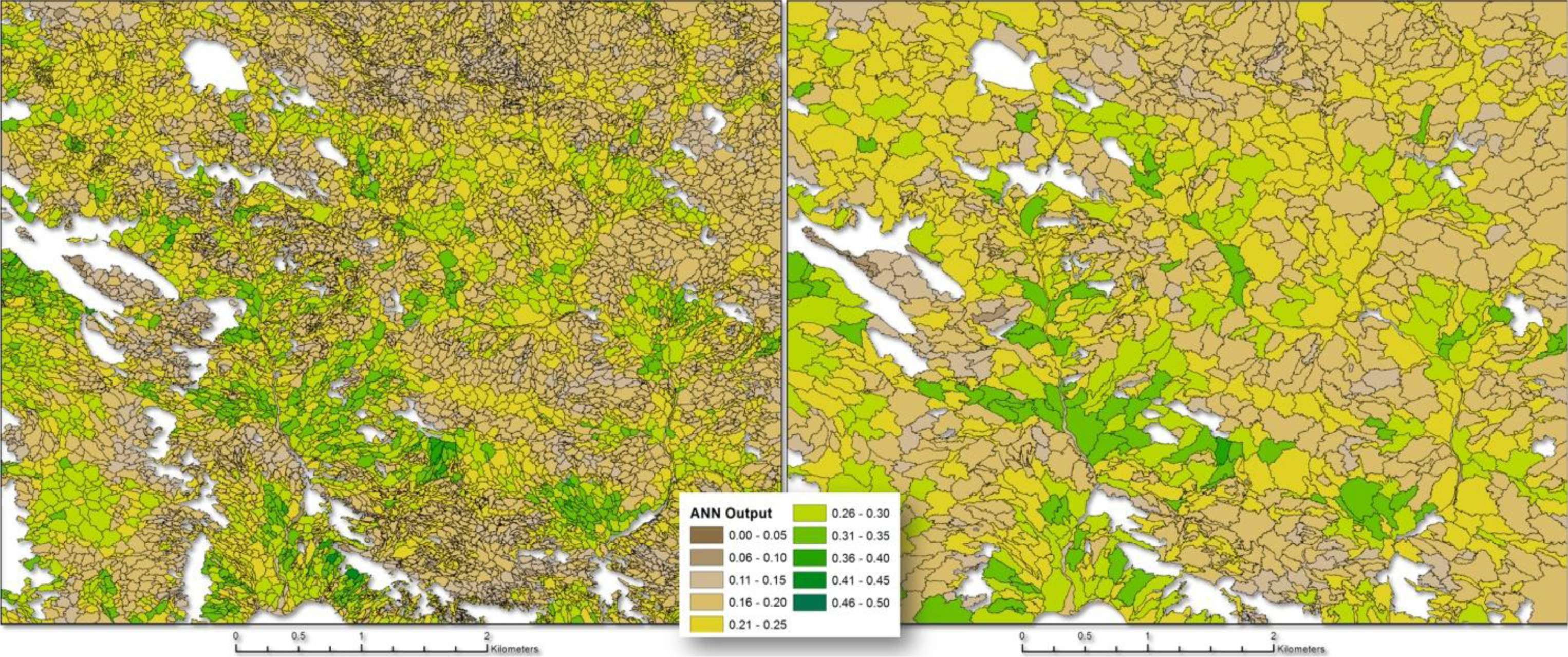
When applied to the larger image objects, the separate eco-class ANNs give similar results to those seen for the smaller image objects for the separate ecological classes, with the combined model results showing an even stronger relationship than for the smaller objects (Table 5, Figure 6). This is likely due to the reduction in extreme values of SAVI and the model output that is a result of increased averaging for the larger image objects. The individual RMSEs are higher than for the small object models, even though the r2 values are higher, a consequence of a much smaller number of image objects: 1333 large objects compared to 10,041 small objects. A smaller number of objects cause the highest and lowest errors to have a greater influence on the overall RMSE. We can also see that the slope of the relationship for the felsenmeer/rock class is lower than the other classes for the large image objects (Figure 6), while it is higher than the other classes for the smaller image objects (Figure 5). This lower slope is due to a lower maximum class SAVI value of 0.18 for the larger objects (versus 0.31 for the smaller objects), again likely an effect of the increased spatial averaging of the larger objects. The visual agreement between the output of the ANNs applied to the different object sizes is also very strong (Figure 7).

Table 5.
Results of the eco-class ANNs when applied to the large image objects.
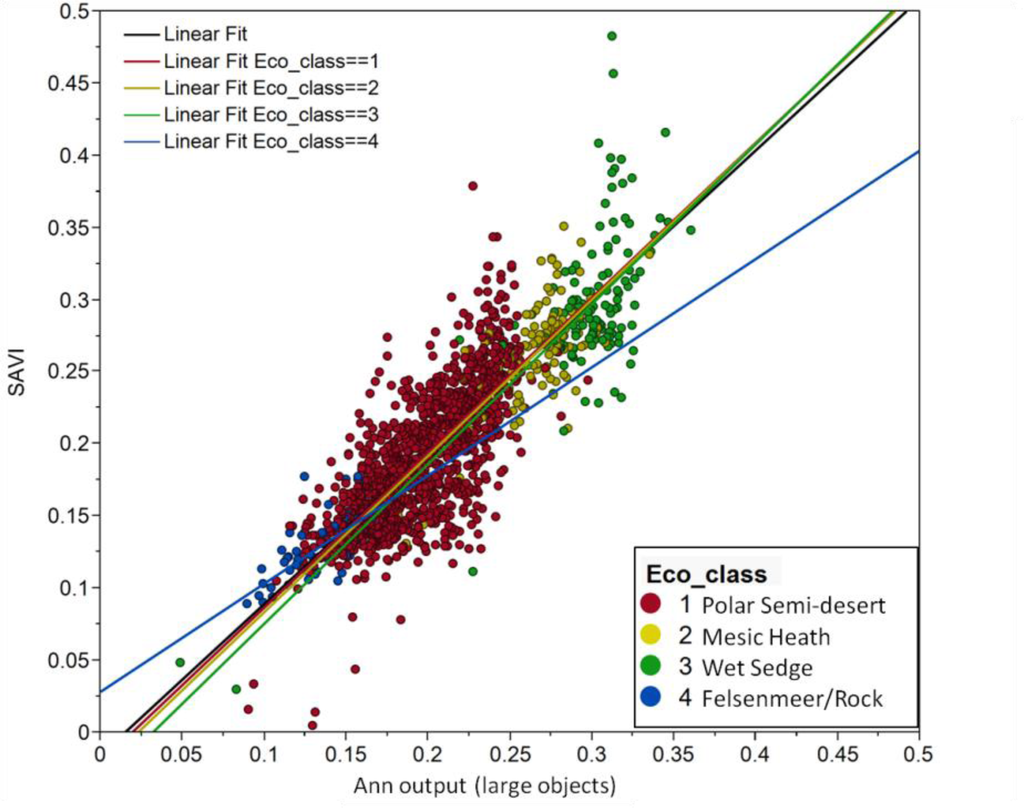
Figure 6.
Regression of the separate eco-class ANNs applied to the larger image objects.
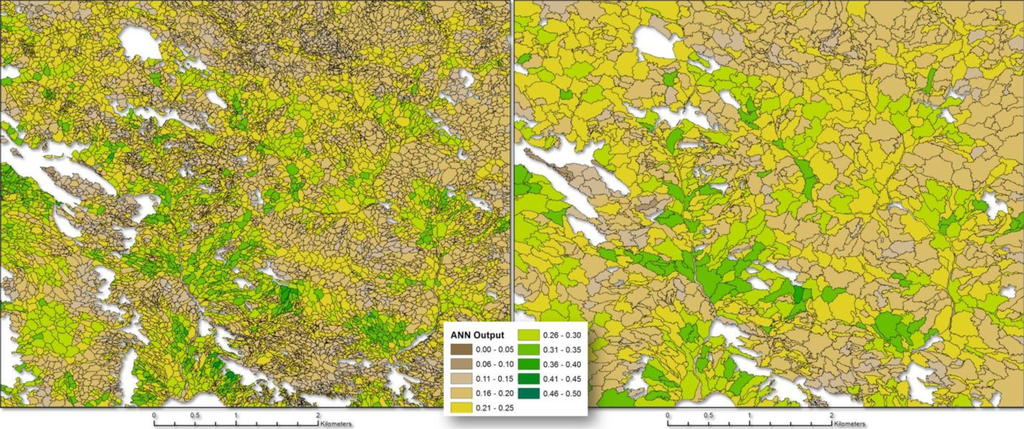
Figure 7.
ANN modeled SAVI output for the Cape Bounty study area when the model is applied to the smaller objects (Left) and the larger objects (Right).
3.3. Above-Ground Phytomass Modeling
The relationship between the ANN-modeled SAVI values and field-measured above-ground phytomass at the Cape Bounty location using the smaller image objects shows a stronger relationship than the previous NDVI-above-ground phytomass relationship of Atkinson and Treitz [9] (Figure 8), with an r2 of 0.87, and a RMSE of 239 g/m2, or approximately 11% of the maximum range of phytomass values. It is not clear whether this improved result is due to the better relationship of SAVI versus NDVI to above-ground phytomass, or if the SAR data is simply more sensitive to above-ground phytomass than the optical vegetation indices. When a similar regression is applied between optical-based SAVI values and above-ground phytomass, the relationship is not quite as strong, with an r2 of 0.79 and a RMSE of 309 g/m2 (approximately 14% of the maximum range of phytomass values), suggesting that the SAR data could be more sensitive to above-ground phytomass. A limitation of this relationship is that it does not hold for values of SAVI less than about 0.1, which in this instance only results in the exclusion of approximately 25 (less than 0.3%) of the image objects. Values of SAVI less than 0.1, represent areas that have extremely low values of above-ground phytomass. The modeled values of above-ground phytomass were then used to create a spatially explicit map of above-ground phytomass across the Cape Bounty study area (Figure 9). A further complication of this relationship arises due to the physical linkage between phytomass and soil moisture in this environment. It is possible that the SAR model is sensitive to the combined moisture/vegetation signal, rather than just vegetation, though this may not be problematic because of the very real relationship between these variables on the ground [9]. Surface roughness can also have a large impact on SAR backscatter values, but controlling for surface roughness values across the landscape (from [60]) did not result in significant changes to the model, suggesting that surface roughness is not a major factor in this instance.
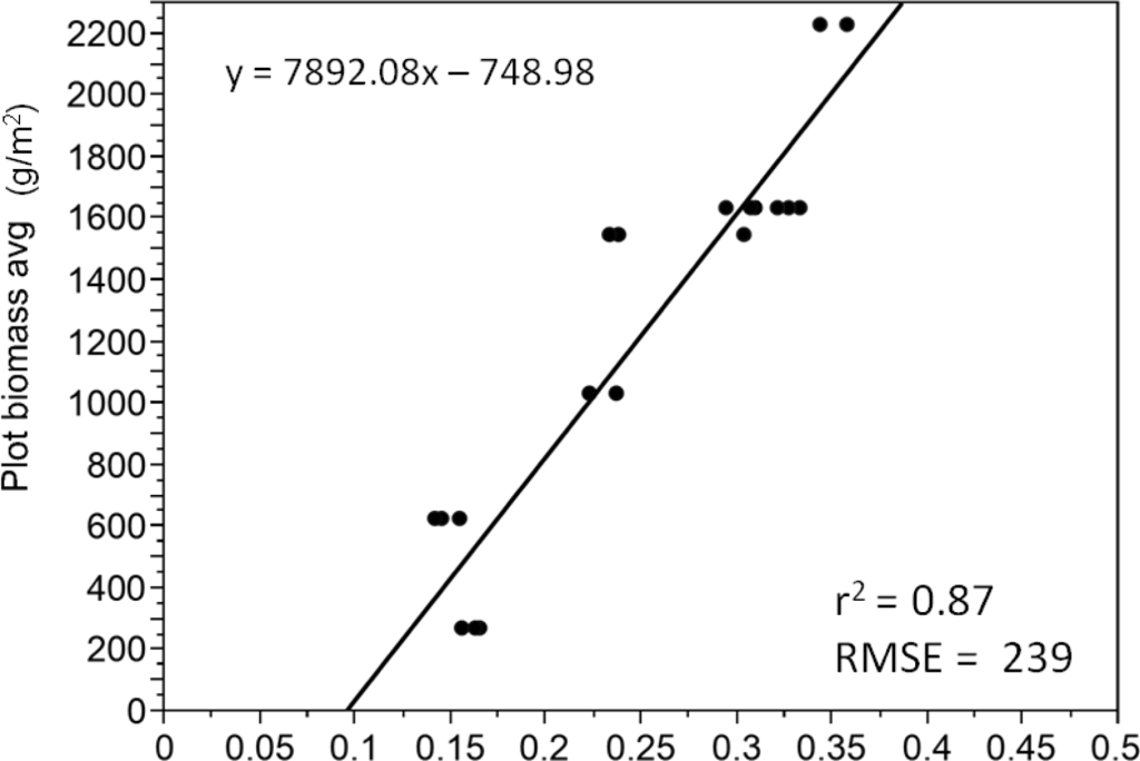
Figure 8.
Relationship between the ANN modeled SAVI values and field-derived measures of above-ground phytomass for the smaller image objects.
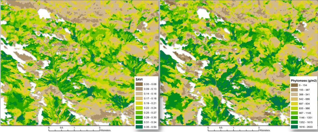
Figure 9.
Multi-spectral derived SAVI values (Left) for the small image objects compared to the SAR-modeled above-ground phytomass values (Right) across the Cape Bounty study area. Blank (white) areas indicate where objects were excluded from the analysis (see methods).
4. Conclusions
High resolution optical data were used to facilitate the modeling of above-ground phytomass using RADARSAT-2 Synthetic Aperture Radar (SAR) data. Three different SAR parameters, along with a topographic position index derived from a high-resolution digital elevation model, were used to create Artificial Neural Network (ANN) models that estimated values of the Soil Adjusted Vegetation Index (SAVI) across different sets of image objects. Models for individual ecological classes were found to outperform a single model that included all classes (r2 = 0.49, normalized root mean square error (N_RMSE) = 9%) when the output from the separate models were combined and compared to the optical-derived SAVI values (r2 = 0.60, N_RMSE = 8%). The models were applied to larger image objects, with acceptable results (r2 = 0.72, N_RMSE = 6%), showing the potential of the models to be applied at multiple spatial scales without sacrificing accuracy. The output of the ANNs was also used to create another model that estimates above-ground phytomass across the landscape, and resulted in a strong relationship with ground-sampled phytomass values (r2 = 0.87, N_RMSE = 11%). This relationship demonstrates the utility of SAR data, compared to using optical data alone, when attempting to model above-ground phytomass in a high arctic environment with relatively low levels of vegetation. The phytomass levels in this environment are low enough that much of the relationship between field-measured phytomass and the SAR variables could be due to backscatter sensitivity to soil moisture, and, to a smaller degree, surface roughness. However, the close coupling of moisture and phytomass in this environment means that this relationship increases rather than decreases the effectiveness of the modeling effort.
Polarimetric variables were not found to be correlated to SAVI, and were therefore not used as inputs to the ANN models. This lack of correlation is not surprising, as the RADARSAT-2 dataset was initially acquired for soil moisture estimation, where steep incidence angles are preferred to reduce the surface roughness dependency and vegetation interaction. In the near future, it would be worthwhile to acquire polarimetric SAR data at shallower incidence angles to maximize vegetation interaction and determine the potential degree of polarimetric C-band SAR correlation to high arctic vegetation. The use of shorter wavelength SAR sensors, such as TerraSAR-X, would also likely increase the effective influence of vegetation on backscatter, due to the very low levels of vegetation in high arctic environments, and is an avenue worth further exploration.
Acknowledgments
This study received RADARSAT-2 data through the Science and Operational Applications Research—Education initiative (SOAR-E) program of the Canadian Space Agency and the Canada Centre for Remote Sensing. Funding was provided by a variety of sources, including a NSERC Alexander Graham Bell Canada Graduate Scholarship (CGS D) (Collingwood), a NSERC IPY Grant (Dr. Scott Lamoureux, PI), a NSERC Discovery Grant (Treitz), ArcticNet, the Northern Scientific Training Program (NSTP), and the Polar Continental Shelf Project (PCSP). RADARSAT-2 Data and Product© MacDonald, Dettwiler and Associates Ltd. (2013)—All Rights Reserved.
Author Contributions
A. Collingwood wrote the manuscript, and was responsible for the design, implementation, and analysis of the research. P. Treitz provided guidance on research design and other details both large and small. F. Charbonneau provided guidance on SAR-specific data processing and management. D.M. Atkinson provided vegetation and biomass data, and lent his expertise in this area. All authors helped with initial manuscript editing.
Conflicts of Interest
The authors declare no conflict of interest.
References
- Walker, D.A.; Epstein, H.E.; Raynolds, M.K.; Kuss, P.; Kopecky, M.A.; Frost, G.V.; Daniëls, F.J.A.; Leibman, M.O.; Moskalenko, N.G.; Matyshak, G.V.; et al. Environment, vegetation and greenness (NDVI) along the North America and Eurasia Arctic transects. Environ. Res. Lett 2012, 7. [Google Scholar] [CrossRef]
- Raynolds, M.K.; Walker, D.A.; Maier, H.A. NDVI patterns and phytomass distribution in the circumpolar Arctic. Remote Sens. Environ 2006, 102, 271–281. [Google Scholar]
- Boelman, N.T.; Stieglitz, M.; Rueth, H.M.; Sommerkorn, M.; Griffin, K.L.; Shaver, G.R.; Gamon, J.A. Response of NDVI, biomass, and ecosystem gas exchange to long-term warming and fertilization in wet sedge tundra. Oecologia 2003, 135, 414–421. [Google Scholar]
- Shaver, G.R.; Street, L.E.; Rastetter, E.B.; van Wijk, M.T.; Williams, M. Functional convergence in regulation of net CO2 flux in heterogeneous tundra landscapes in Alaska and Sweden. J. Ecol 2007, 95, 802–817. [Google Scholar]
- Torn, M.S.; Chapin, F.S. Environmental and biotic controls over methane flux from arctic tundra. Chemosphere 1993, 26, 357–368. [Google Scholar]
- Parker, G.R.; Ross, R.K. Summer habitat use by muskoxen (ovibos moschatus) and peary caribou (rangifer tarandus pearyi) in the Canadian High Arctic. Polarforschung 1975, 1, 12–25. [Google Scholar]
- Abuelgasim, A.A.; Leblanc, S.G. Leaf area index mapping in northern Canada. Int. J. Remote Sens 2011, 32, 5059–5076. [Google Scholar]
- Laidler, G.J.; Treitz, P.M.; Atkinson, D.M. Remote sensing of arctic vegetation: Relations between the NDVI, spatial resolution and vegetation cover on boothia peninsula, nunavut. Arctic 2008, 61, 1–13. [Google Scholar]
- Atkinson, D.M.; Treitz, P. Modeling biophysical variables across an arctic latitudinal gradient using high spatial resolution remote sensing data. Arctic Antarct. Alp. Res 2013, 45, 161–178. [Google Scholar]
- Shaver, G.R.; Chapin, F.S.I. Response to fertilization by various plant growth forms in an alaskan tundra: nutrient accumulation and growth. Ecology 1980, 61, 662–675. [Google Scholar]
- Van Wijk, M.T.; Williams, M.; Shaver, G.R. Tight coupling between leaf area index and foliage N content in arctic plant communities. Oecologia 2005, 142, 421–427. [Google Scholar]
- Billings, W.D. Arctic and alpine vegetations: Similarities, differences, and susceptibility to disturbance. Bioscience 1973, 23, 697–704. [Google Scholar]
- Evans, B.M.; Walker, D.A.; Benson, C.S.; Nordstrand, E.A.; Petersen, G.W. Spatial interrelationships between terrain, snow distribution and vegetation patterns at an arctic foothills site in Alaska. Ecography 1989, 12, 270–278. [Google Scholar]
- Walker, D.A.; Kuss, P.; Epstein, H.E.; Kade, A.N.; Vonlanthen, C.M.; Raynolds, M.K.; Daniëls, F.J.A. Vegetation of zonal patterned-ground ecosystems along the North America Arctic bioclimate gradient. Appl. Veg. Sci 2011, 14, 440–463. [Google Scholar]
- Sitch, S.; McGuire, A.D.; Kimball, J.; Gedney, N.; Gamon, J.; Engstrom, R.; Wolf, A.; Zhuang, Q.; Clein, J.; McDonald, K.C. Assessing the carbon balance of circumpolar Arctic tundra using remote sensing and process modeling. Ecol. Appl 2007, 17, 213–234. [Google Scholar]
- Williams, M.; Bell, R.; Spadavecchia, L.; Street, L.E.; van Wijk, M.T. Upscaling leaf area index in an Arctic landscape through multiscale observations. Glob. Chang. Biol 2008, 14, 1517–1530. [Google Scholar]
- Loranty, M.M.; Goetz, S.J.; Rastetter, E.B.; Rocha, A.V; Shaver, G.R.; Humphreys, E.R.; Lafleur, P.M. Scaling an instantaneous model of tundra nee to the arctic landscape. Ecosystems 2011, 14, 76–93. [Google Scholar]
- Barrett, B.W.; Dwyer, E.; Whelan, P. Soil moisture retrieval from active spaceborne microwave observations: An evaluation of current techniques. Remote Sens 2009, 1, 210–242. [Google Scholar]
- Bindlish, R.; Barros, A.P. Parameterization of vegetation backscatter in radar-based, soil moisture estimation. Remote Sens. Environ 2001, 76, 130–137. [Google Scholar]
- Trudel, M.; Charbonneau, F.; Leconte, R. Using RADARSAT-2 polarimetric and ENVISAT-ASAR dual-polarization data for estimating soil moisture over agricultural fields. Can. J. Remote Sens 2012, 38, 1–14. [Google Scholar]
- Paloscia, S.A. Summary of experimental results to assess the contribution of SAR for mapping vegetation biomass and soil moisture. Can. J. Remote Sens 2002, 28, 246–261. [Google Scholar]
- Mattia, F.; Le Toan, T.; Picard, G.; Posa, F.I.; D’Alessio, A.; Notarnicola, C.; Gatti, A.M.; Rinaldi, M.; Satalino, G.; Pasquariello, G. Multitemporal C-band radar measurements on wheat fields. IEEE Trans. Geosci. Remote Sens 2003, 41, 1551–1560. [Google Scholar]
- Morrissey, L.A.; Livingston, G.P.; Durden, S.L. Use of SAR in regional methane exchange studies. Int. J. Remote Sens 1994, 15, 1337–1342. [Google Scholar]
- Moran, M.S.; Peters-Lidard, C.D.; Watts, J.M.; McElroy, S. Estimating soil moisture at the watershed scale with satellite-based radar and land surface models. Can. J. Remote Sens 2004, 30, 805–826. [Google Scholar]
- McNairn, H.; Hochheim, K.; Rabe, N. Applying polarimetric radar imagery for mapping the productivity of wheat crops. Can. J. Remote Sens 2004, 30, 517–524. [Google Scholar]
- Smith, A.M.; Buckley, J.R. Investigating RADARSAT-2 as a tool for monitoring grassland in western Canada. Can. J. Remote Sens 2011, 37, 93–102. [Google Scholar]
- Ulaby, F.T.; Moore, R.K.; Fung, K.A. Microwave Remote Sensing: Active and Passive. In Theory to Applications; Artech House, Inc.: Dedham, MA, USA, 1986; Volume 3. [Google Scholar]
- Kim, Y.; van Zyl, J.J.A. Time-series approach to estimate soil moisture using polarimetric radar data. IEEE Trans. Geosci. Remote Sens 2009, 47, 2519–2527. [Google Scholar]
- Moran, M.S.; Hymer, D.C.; Qi, J.; Sano, E.E. Soil moisture evaluation using multi-temporal synthetic aperture radar (SAR) in semiarid rangeland. Agric. For. Meteorol 2000, 105, 69–80. [Google Scholar]
- Sano, E.E.; Huete, A.R.; Troufleau, D.; Moran, M.S.; Vidal, A. Relation between ERS-1 synthetic aperture radar data and measurements of surface roughness and moisture content of rocky soils in a semiarid rangeland. Water Resour. Res 1998, 34, 1491–1498. [Google Scholar]
- Gross, M.F.; Hardisky, M.A.; Doolittle, J.A.; Klemas, V. Relationships among depth to frozen soil, soil wetness, and vegetation type and biomass in Tundra near Bethel, AK, USA. Arct. Alp. Res 1990, 22, 275–282. [Google Scholar]
- Meade, N.G.; Hinzman, L.D.; Kane, D.L. Spatial estimation of soil moisture using synthetic aperture radar in Alaska. Adv. Sp. Res 1999, 24, 935–940. [Google Scholar]
- Sahebi, M.R.; Bonn, F.; Bénié, G.B. Neural networks for the inversion of soil surface parameters from synthetic aperture radar satellite data. Can. J. Civ. Eng 2004, 31, 95–108. [Google Scholar]
- Said, S.; Kothyari, U.C.; Arora, M.K. ANN-Based soil moisture retrieval over bare and vegetated areas using ERS-2 SAR data. J. Hydrol. Eng 2008, 13, 461–475. [Google Scholar]
- Del Frate, F.; Wang, L. Sunflower biomass estimation using a scattering model and a neural network algorithm. Int. J. Remote Sens 2001, 22, 1235–1244. [Google Scholar]
- Mas, J.F.; Flores, J.J. The application of artificial neural networks to the analysis of remotely sensed data. Int. J. Remote Sens 2008, 29, 617–663. [Google Scholar]
- Raynolds, M.K.; Walker, D.A.; Epstein, H.E.; Pinzon, J.E.; Tucker, C.J.A. New estimate of tundra-biome phytomass from trans-Arctic field data and AVHRR NDVI. Remote Sens. Lett 2012, 3, 403–411. [Google Scholar]
- Gregory, F.M. Biophysical Remote Sensing and Terrestrial CO2 Exchange at Cape Bounty, Melville Island; Queen’s University: Kingston, ON, Canada, 2011; p. 161. [Google Scholar]
- Tenhunen, J.D.; Lange, O.L.; Hahn, S.; Siegwolf, R.; Oberbauer, S.F. The Ecosystem Role of Poikilohydric Tundra Plants. In Arctic Ecosystems in a Changing Climate; Chapin, F.S.I., Jefferies, R.L., Reynolds, J.F., Shaver, G.R., Svoboda, J., Eds.; Academic Press: San Diego, CA, USA, 1992; pp. 213–237. [Google Scholar]
- Douma, J.C.; van Wijk, M.T.; Lang, S.I.; Shaver, G.R. The contribution of mosses to the carbon and water exchange of arctic ecosystems: Quantification and relationships with system properties. Plant. Cell Environ 2007, 30, 1205–1215. [Google Scholar]
- Harris, A. Spectral reflectance and photosynthetic properties of sphagnum mosses exposed to progressive drought. Ecohydrology 2008, 1, 35–42. [Google Scholar]
- Bubier, J.L.; Rock, B.N.; Crill, P.M. Spectral reflectance measurements of boreal wetland and forest mosses. J. Geophys. Res 1997, 102, 29483–29494. [Google Scholar]
- Watanabe, M.; Kadosaki, G.; Kim, Y.; Ishikawa, M.; Kushida, K.; Sawada, Y.; Tadono, T.; Fukuda, M.; Sato, M. Analysis of the sources of variation in L-band backscatter from terrains with permafrost. IEEE Trans. Geosci. Remote Sens 2012, 50, 44–54. [Google Scholar]
- Huete, A.R. A soil-adjusted vegetation index (SAVI). Remote Sens. Environ 1988, 25, 295–309. [Google Scholar]
- Atkinson, D.M.; Treitz, P. Arctic ecological classifications derived from vegetation community and satellite spectral data. Remote Sens 2012, 4, 3948–3971. [Google Scholar]
- Hodgson, D.A.; Vincent, J.-S. A 10,000 yr B.P. extensive ice shelf over viscount melville sound, arctic Canada. Quat. Res 1984, 22, 18–30. [Google Scholar]
- Lajeunesse, P.; Hanson, M.A. Field observations of recent transgression on northern and eastern Melville Island, western Canadian Arctic Archipelago. Geomorphology 2008, 101, 618–630. [Google Scholar]
- CAVM Team. Circumpolar Arctic Vegetation Map, scale 1: 7,500,000; Conservation of Arctic Flora and Fauna (CAFF) Map No. 1; CAVM Team: Anchorage, AK, USA, 2003. [Google Scholar]
- Guisan, A.; Weiss, S.B.; Weiss, A.D. GLM versus CCA spatial modeling of plant species distribution. Plant Ecol 1999, 143, 107–122. [Google Scholar]
- Jenness, J.; Brost, B.; Beier, P. Land Facet Corridor Designer: Extension for ArcGIS. Available online: http://www.jennessent.com/arcgis/land_facets.htm (accessed on 7 March 2014).
- Blaschke, T. Object based image analysis for remote sensing. ISPRS J. Photogramm. Remote Sens 2010, 65, 2–16. [Google Scholar]
- Drăguţ, L.; Schauppenlehner, T.; Muhar, A.; Strobl, J.; Blaschke, T. Optimization of scale and parametrization for terrain segmentation: An application to soil-landscape modeling. Comput. Geosci 2009, 35, 1875–1883. [Google Scholar]
- Draˇguţ, L.; Tiede, D.; Levick, S.R. ESP: A tool to estimate scale parameter for multiresolution image segmentation of remotely sensed data. Int. J. Geogr. Inf. Sci 2010, 24, 859–871. [Google Scholar]
- Cloude, S.R.; Pottier, E. An entropy based classification scheme for land applications of polarimetric SAR. IEEE Trans. Geosci. Remote Sens 1997, 35, 68–78. [Google Scholar]
- Haralick, R.M.; Shanmugam, K.; Dinstein, I. Textural features for image classification. IEEE Trans. Syst. Man. Cybern 1973, SMC-3, 610–621. [Google Scholar]
- Oliver, C.; Quegan, S. Understanding Synthetic Aperture Radar Images; Arteck House: Boston, MA, USA, 1998; p. 479. [Google Scholar]
- Sahebi, M.R.; Angles, J.; Bonn, F.A. Comparison of multi-polarization and multi-angular approaches for estimating bare soil surface roughness from spaceborne radar data. Can. J. Remote Sens 2002, 28, 641–652. [Google Scholar]
- Hagan, M.T.; Menhaj, M.B. Training feedforward networks with the marquardt algorithm. IEEE Trans. Neural Netw 1994, 5, 989–993. [Google Scholar]
- Epstein, H.E.; Raynolds, M.K.; Walker, D.A.; Bhatt, U.S.; Tucker, C.J.; Pinzon, J.E. Dynamics of aboveground phytomass of the circumpolar Arctic tundra during the past three decades. Environ. Res. Lett 2012, 7. [Google Scholar] [CrossRef]
- Collingwood, A.; Treitz, P.; Charbonneau, F. Surface roughness estimation from RADARSAT-2 data in a High Arctic environment. Int. J. Appl. Earth Obs. Geoinf 2014, 27, 70–80. [Google Scholar]
© 2014 by the authors; licensee MDPI, Basel, Switzerland This article is an open access article distributed under the terms and conditions of the Creative Commons Attribution license (http://creativecommons.org/licenses/by/3.0/).

