Article

Mapping Spatial Distribution of Larch Plantations from Multi-Seasonal Landsat-8 OLI Imagery and Multi-Scale Textures Using Random Forests

1
State Key Laboratory of Forest and Soil Ecology, Institute of Applied Ecology, Chinese Academy of Sciences, Shenyang 110016, China
2
Qingyuan Forest CERN, Chinese Academy of Sciences, Shenyang 110016, China
3
University of Chinese Academy of Sciences, Beijing 110164, China
4
Key Laboratory of Agri-informatics, Ministry of Agriculture / Institute of Agricultural Resources and Regional Planning, Chinese Academy of Agricultural Sciences, Beijing 100081, China
*
Author to whom correspondence should be addressed.
Remote Sens. 2015, 7(2), 1702-1720; https://doi.org/10.3390/rs70201702
Submission received: 16 October 2014 / Revised: 23 December 2014 / Accepted: 29 January 2015 / Published: 5 February 2015

Abstract

:
The knowledge about spatial distribution of plantation forests is critical for forest management, monitoring programs and functional assessment. This study demonstrates the potential of multi-seasonal (spring, summer, autumn and winter) Landsat-8 Operational Land Imager imageries with random forests (RF) modeling to map larch plantations (LP) in a typical plantation forest landscape in North China. The spectral bands and two types of textures were applied for creating 675 input variables of RF. An accuracy of 92.7% for LP, with a Kappa coefficient of 0.834, was attained using the RF model. A RF-based importance assessment reveals that the spectral bands and bivariate textural features calculated by pseudo-cross variogram (PC) strongly promoted forest class-separability, whereas the univariate textural features influenced weakly. A feature selection strategy eliminated 93% of variables, and then a subset of the 47 most essential variables was generated. In this subset, PC texture derived from summer and winter appeared the most frequently, suggesting that this variability in growing peak season and non-growing season can effectively enhance forest class-separability. A RF classifier applied to the subset led to 91.9% accuracy for LP, with a Kappa coefficient of 0.829. This study provides an insight into approaches for discriminating plantation forests with phenological behaviors.

Graphical Abstract

1. Introduction

Natural forests have been destroyed for more than a century worldwide due to human activity, and plantation forests are planted to meet the demand of timber as a substitution for natural forests [1]. Accounting for 36% of the country’s total forested area, China possesses the largest area of planted forests (PF) in the world [2]. Larix spp. is one of the most important planted timber tree species. Since the 1950s, about 3.78 million ha of larch plantations (LP) have been planted in North China, which provides essential ecosystem services, including timber production, water resource conservation and carbon sequestration [3]. With a continuing increase in planted LP area, some problems have been reported regarding LPs such as the poor natural regeneration capability [4,5], and a decline in soil fertility [6,7]. The knowledge about spatial patterns of LP is of prime importance to forest management, monitoring programs and ecological services functional assessment, which services for the strategic goals of managing plantation forests [1,8,9]. Nevertheless, due to the extensive area and long-period of planting LPs in North China, its spatial distribution pattern remains unclear.
Remote sensing is particularly useful for forest mapping, as it provides a large coverage at relatively high levels of detail [10,11,12,13,14]. Nevertheless, for specific tree species during mono-temporal stage (e.g., growing season), an accurate remote sensing-based classification is still particularly challenging, as the spectral signal from trees may be very hard to distinguish from one another. Multi-seasonal remote sensing images are used to introduce temporal variability of objects as a feature to increase class-separability [15,16,17]. In the process of global land-cover mapping, for example, Gong et al. found multi-temporal Landsat images useful in investigating land-cover classification [18]. This multi-temporal images-based classification has been applied to map land cover [17,19], wetlands [16] and forest biomass [20]. Although this idea has received increasing interest, the multi-seasonal imagery-based classification that allows for the separation of different forest types, is still lacking.
The spatial variability of vegetation cover patterns can be incorporated into the mapping process to distinguish objects more effectively [17,21]. Image texture, which describes the visual spatial variability, has been widely used in identifying vegetation types [22,23]. Various texture measures aiming to quantify smoothness, symmetry, regularity, etc., of an image have been developed based on the grey level co-occurrence matrix (GLCM) and geostatistical functions [24]. Among these texture approaches, the geostatistical approach derived from variogram functions cannot only be calculated for a single image band (univariate mono-seasonal texture), but for a set of bands which describe the covariances between bands of an image for a time series representing different seasons (bivariate multi-seasonal texture). It is especially useful in certain situations where the seasonal differences between the forest types are important for class discrimination. Larch is a deciduous and coniferous tree species, which has remarkable seasonal changes. In summer, spectral signal from coniferous forest is different from broadleaf forest; in winter, larch shed their leaves and it hereby can be discriminated from the other evergreen coniferous tree species. Furthermore, most of LPs in China are a single species monoculture [5]. These multi-seasonal textures measures may help to extract the seasonal dynamic of pure forests more accurately. However, little attention has been paid to the phenological texture-based classification of forest types.
Although a number of input variables derived from multi-seasonal spectral data and textures can identify features of forest types and improve classifier accuracy, this may lead to the concomitant curse of dimensionality which may be generated due to the application of various transformations to the original satellite images and hinder the expected increase in accuracy related to the inclusion of redundant features [25]. Two methods were used to address this problem: Selecting a robust classifier capable of handling a large number of variables, or selecting only the most informative ones by evaluating individual input variables [17,26]. Random Forests (RF) is an ensemble learning algorithm that has been documented as an excellent performer for the analyses of many complex remote sensing datasets [27,28,29]. It exhibits many desirable properties, including high accuracy, processing thousands of input variables, integrated measures of variable importance, and so on [30,31]. The RF-based variable importance measure can be applied to reduce data dimensionality and further improve classifier efficiency. The previous studies have reported on the RF-based classification approaches with multi-seasonal imageries for land cover mapping [17,19]. However, these studies mostly focused on specific seasons (e.g., spring and summer). For a given forest type discrimination, a time series data set throughout the growing cycle of trees can efficiently identify phenological behaviors of different forest types, thus it may be quite applicable for LP discrimination. Additionally, although the previous studies examined the RF-based importance assessment of remote sensing variables for land cover classification [17,32], the variable applicability for forest type classification is uncertain.
The objectives of this study are to (1) assess performance of the RF learning algorithm in the discrimination of LP; (2) quantify the importance of input variables; (3) map spatial distribution of LP at a local scale. To achieve these goals, multi-seasonal (spring, summer, autumn and winter) Landsat-8 Operational Land Imager (OLI) imageries, texture models and ancillary data were employed to adopt a RF-based feature selection (FS) method. Based on the evaluation of these input variables, a RF classifier was developed to map LP distribution.

2. Materials and Methods
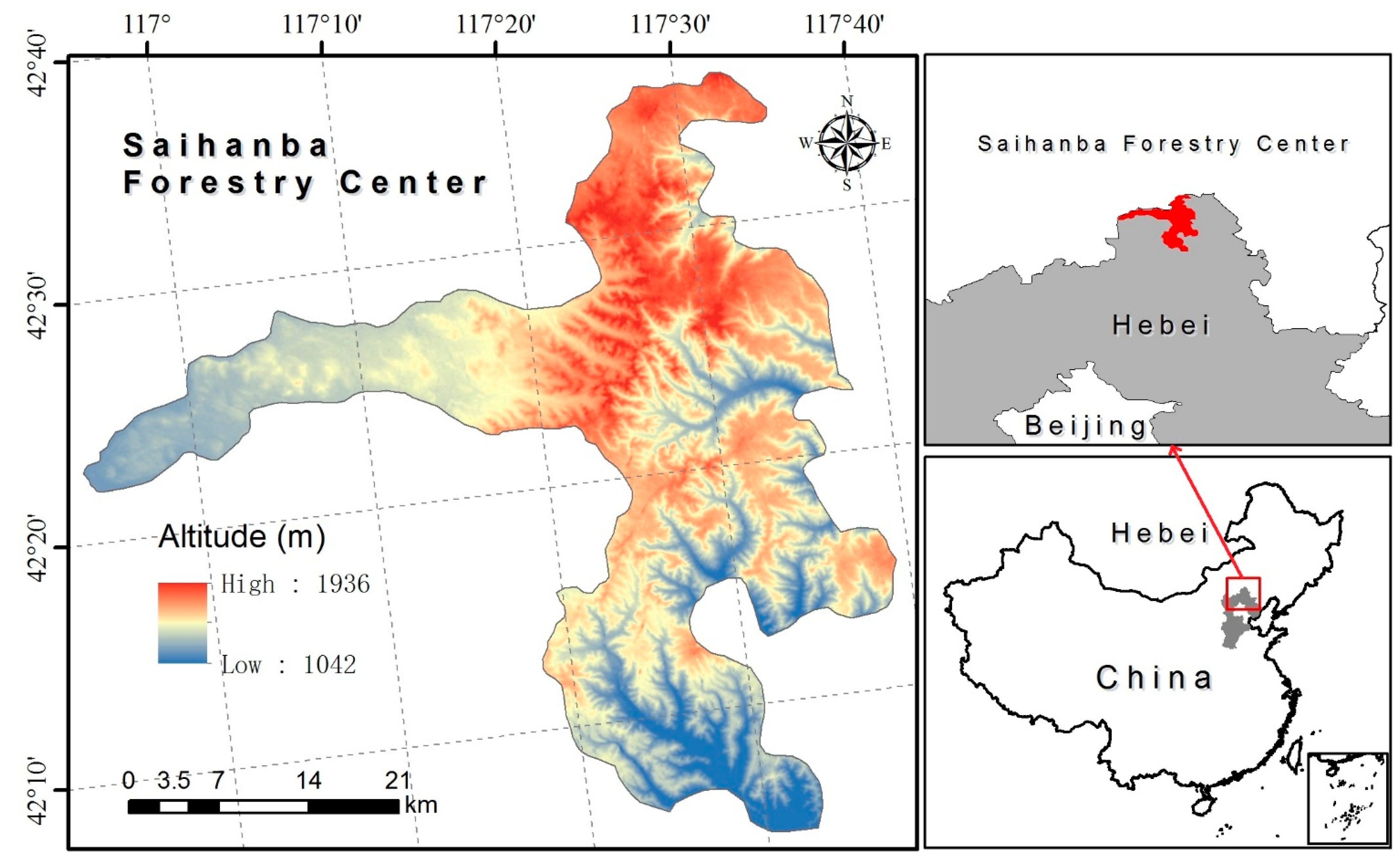
2.1. Study Area

This study was conducted at the Saihanba Forestry Center (SFC) in Hebei Province, Northern China (116°52′E–117°39′E, 42°04′N–42°36′N; ca. 93,000 ha; Figure 1). It is located in the transition between the Inner Mongolian Plateau and North Hebei Mountain, with an elevation ranging from 1042 m to 1936 m. The climate features semi-arid and semi-humid, with a short growing season of May to September. Annual mean air temperature and precipitation were −1.2 °C and 530 mm, respectively. SFC consisted of six sub-forestry centers. Since 1960s, SFC has planted over 74,000 ha of planted forest, which is the largest planted forestry center in China; at present the forest cover of SFC reaches as high as 80%. The main planted forest types are Larix principis-rupprechtii plantations (LP), Pinus sylvestris var. mongolica plantations (MP), Picea asperata plantations (AP) and Pinus tabulaeformis plantations (PP); the main natural secondary tree species is Betula platyphylla forests (BF) and rare hardwood deciduous forests (HDF). SFC is a typical area of plantation forests in Northern China, with forest types consisting of coniferous and deciduous tree species; thus it is a suitable location for investigating LP mapping.
Figure 1. Location of Saihanba Forestry Center.
Remotesensing 07 01702 g001

2.2. Data Acquisition and Preprocessing

Remotely sensed imagery used for this study is Landsat-8 OLI, which is a new sensor of the Landsat series. Landsat-8 extends the Landsat series records and has enhanced capabilities including new spectral bands, improved sensor signal-to-noise performance and associated improvements in radiometric resolution, etc., [33]. In this study, six bands of Landsat-8 were utilized, including OLI2 (blue, 0.45–0.51 μm), OLI3 (green, 0.53–0.59 μm), OLI4 (red, 0.64–0.67 μm), OLI5 (near infrared, 0.85–0.88 μm), OLI6 (shortwave infrared, 1.57–1.65 μm) and OLI7 (shortwave infrared, 2.11–2.29 μm). Four Landsat-8 OLI scenes (Path: 123/Row: 31), captured in spring (green-up stage; 15 May 2014), summer (growing peak stage; 29 July 2013), autumn (defoliating stage; 4 October 2013), and winter (leafless and snowless stage; 4 November 2013), were employed to characterize temporal LP phenological variations.
Geometric correction was performed by approximately 50 ground control points to reduce the error to less than 15 m for the 4-scene Landsat OLI images. Then, atmospheric correction of the images was performed using the Fast Line-of Sight Atmospheric Analysis of Spectral Hypercubes (FLAASH) software package in ENVI 5.0.
Accurate and sufficient training plot data are crucial for a supervised classification. A reference dataset was obtained from forest inventory data of SFC in 2011. The ground data derived from two field surveys in 2013 and high-resolution aerial imagery (0.5 m) from 2012 were applied to verify the reference dataset of SFC; a few polygons (ca. 5% of the total area) were adjusted to obtain an improved ground reference dataset. Then, a random sampling approach was directly used with the improved forest map of SFC. A total of 9909 homogeneous areas were selected to identify forest types to train and test the classifier (Table 1). Each site was confined by a 90 m by 90 m homogeneous area, following recommendations by Congalton and Green [34]. Additionally, the forest map of SFC was also employed as a base forest map for exclusion of the other land covers.
Table 1. The total number of samples for the six forest types LP, Larix principis-rupprechtii plantations; MP, Pinus sylvestris var. mongolica plantations; BF, Betula platyphylla secondary forests; AP, Picea asperata plantations; PP, Pinus tabulaeformis plantations; HDF, hardwood deciduous secondary forests.
IDForest TypeTotal Samples
1LP5831
2BF2912
3MP949
4AP102
5HDF86
6PP29
Total9909
Plantation forests tend to be planted in a flat area, while natural forests distribute in a rugged terrain. Considering the topographic effects on the distribution of forest types, three topographic features were used as input ancillary variables for the RF classifier. Altitude was derived from Shuttle Radar Topography Mission (SRTM) digital elevation models (DEM) raster with a spatial resolution of 30 by 30 m. Slope and aspect were generated from the DEM.

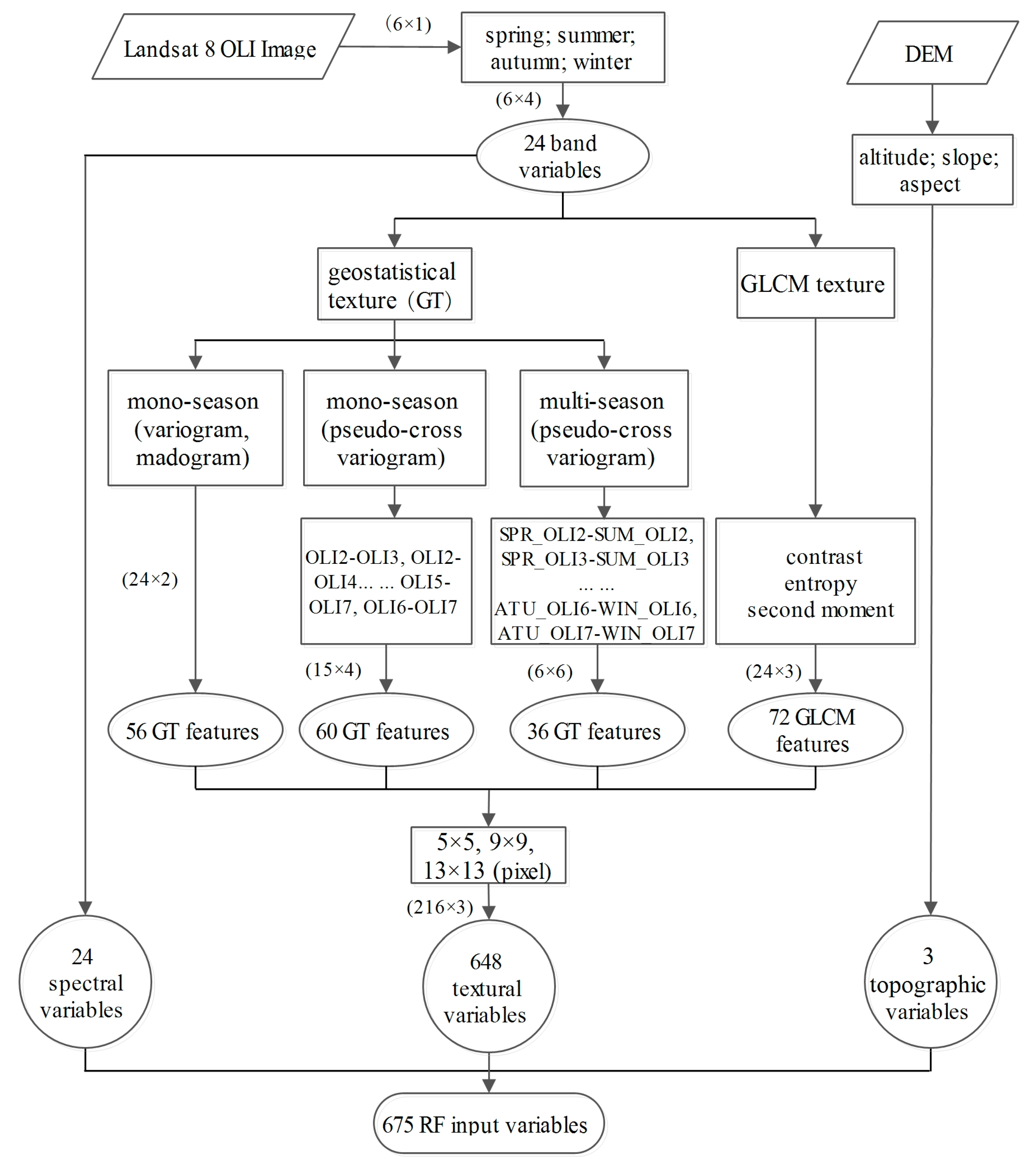
2.3. Textural Analysis

Image texture carries useful information for discriminating forest types. The multi-scale textural features which combined geostatistical texture and GLCM texture, were calculated from Landsat-8 multi-seasonal OLI bands (band 2 to band 7) to introduce textural variables into the LP discrimination. It should be noted that selection of the window size is a practical problem, depending on the spatial resolution of the image and the characteristics of the land cover [17,24,35]. The proper window size can ensure obtaining a robust textural estimator. Rodriguez-Galiano et al. [17] suggested that a small window size provide a more representative description of the most heterogeneous environments with high local variance, while larger window sizes may provide an accurate representation of a homogeneous pattern of spatial variability of large areas. By referring to the previous studies and considering patch size of forest in SFC, three different window sizes were tested, including 5 × 5 pixels (150 × 150 m), 9 × 9 pixels (270 × 270 m) and 13 × 13 pixels (390 × 390 m).

2.3.1. Geostatistical Texture

The geostatistics approach is a textural analysis tool used to measure spatial variation (e.g., spatial autocorrelation) in remotely sensed data [36]. Implementation of variograms is one of the most promising techniques of geostatistics and it has been widely used in image texture characterization [37]. It can be applied not only to calculate the texture contrast within a single spectral band (univariate analysis) but also to describe the relationships between pairs of spectral bands (bivariate analysis) [32]. For the latter, the bivariate analyses can be performed with two bands of mono-season or same band of coupled seasons. In order to identify characters of LP in SFC, three geostatistical measures (variogram, madogram and pseudo-cross variogram) were applied to mono-seasonal and multi-seasonal images. The direction of variogram computation and the lag distance h are the two important parameters affecting texture values. In this study, the four main directions (N–S, E–W, NE–SW and NW–SE) were averaged to produce an omnidirectional variogram texture [36,37]. Because different lag distances have a limited effect on classification results [17,32], one lag (h = 1) were selected for the three window sizes. More detailed descriptions about variogram functions and definitions of parameters can be found in previous studies [36,37,38]. All the prediction variables derived from geostatistical texture were showed in Figure 2.

2.3.2. GLCM Texture

GLCM is an alternative texture analysis tool, which is widely used to describe the specific textural characteristics of an image [39]. This texture features calculated from a matrix containing relative occurrence frequencies gray level (digital numbers) of pairs of pixels at a fixed relative position in an image [22,32]. Similarly, some parameters should be defined to process the calculation of GLCM texture. For explanation of the GLCM parameters (window sizes, lag distance and orientation), refer to the definition of geostatistical textures (Section 2.3.1). There are a variety of GLCM measures employed in current studies. In order to avoid correlation between textural features as well as reduce data dimensionality, we referred Coburn et al. study and selected the three GLCM measures [39]. The defined parameters and texture features of GLCM are shown in Figure 2.

2.4. Random Forests Classification and Feature Selection

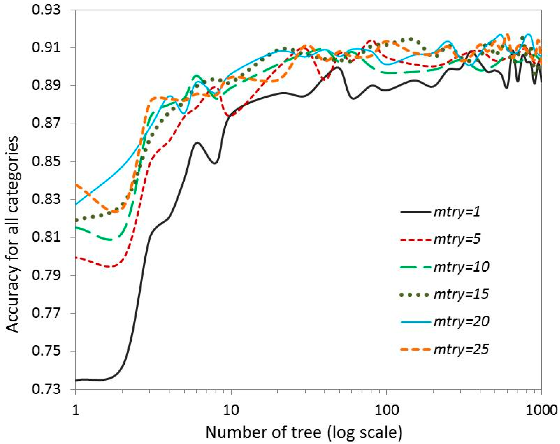
2.4.1. Random Forests Classifier

The machine learning technique RF is an improved version of the Classification and Regression Tree that can be viewed as an ensemble of individual tree-like classifiers [27,40]. RF algorithm shows neither sensitivity to noise nor overfitting than other classifiers based on bagging or boosting [32,41]. It can handle a thousand of input variables and evaluate their importance in classification [27]. In this study, a RF classifier was used to discriminate LP from the other forest types and estimate the importance of 675 input variables.
In a process of RF classification, two basic parameters are required to generate a prediction model, the number of trees in a forest (ntree) and the number of prediction variables for use at each split to grow a decision tree (mtry). Although Breiman [27] suggested that adding more trees to RF model does not induce over-training, redundant trees can introduce the increase of computational time. For a number of prediction variables, its reduction causes a less robust individual tree, while reduces the correlation between trees, which increases the classifier accuracy [42]. Therefore, the parameters of the RF model should be optimized for obtaining a high-efficient RF classifier. Considering computation time of RF, ntree is set to the upper limit of 1000. A number of RF models based on possible values of ntree and mtry were created and evaluated to analyze the effect of the two parameters on classification accuracy. The optimal parameters would be applied to improve the RF classifier efficiency.
Figure 2. Flowchart describing the process of calculating the input variables of RF classifier. The total 675 potential variables consisted of spectral bands, textual variables and topographic data. The six bands of multi-seasonal OLI images and topographic variable (altitude, slope and aspect) derived from DEM were directly utilized as RF input variables. For geostatistical textures (GT), both mono-seasonal (univariate and bivariate) and multi-seasonal (bivariate) images were employed. The mono-seasonal GTs were calculated by single band (variogram and madogram, 24 bands × 2 GTs) and pair of bands (pseudo-cross variogram, 15 band combinations × 4 seasons); multi-seasonal GT was calculated by single band for different combinations of coupled seasons (6 bands × 6 seasonal combinations). All the texture variables were generated by omnidirection (averaged by the four main directions), one lag distance (h = 1) and different scales (window sizes equal to 5 × 5 pixels, 9 × 9 pixels and 13 × 13 pixels).
Remotesensing 07 01702 g002
The ground reference data (Table 1) was divided randomly into 70% and 30% for training and testing of RF model, respectively (Section 2.2), which the number of training sites per class was kept roughly equal [17]. A confusion matrix was generated to assess classification accuracy.

2.4.2. Feature Selection

The three kinds of data which derived from original satellite spectral bands, textural measures and topographic data produced 675 predictive variables for RF (Figure 2). The original spectral variables are informative and often been directly used in remote sensing-based classification [26,43]. Additionally, in order to identify the monoculture and phenological behaviors of LP, two textural methods (GLCM and geostatistical texture) were employed. Since textual measures with multiple parameter combinations (e.g., window size, direction or lag) can dramatically increase variables, many efforts have been carried out to reduce the data dimensionality (Section 2.3).
The textural variables may increase the classification accuracy, but these variables may highly correlate sometimes as well as generate an excess of computational time and the “curse of dimensionality” [25]. It is important to know how each predictive variable influences the RF model and further identify the efficiency of variables for LP discrimination. An assessment of variable importance produced by the RF model can help to select the more effective variables with little reduction in classification accuracy. In this process, by random permuting of values of the variable in the out-of-bag (OOB) samples, the increase of estimation error for the modified and original OOB data is measured for determining the variable importance [44]. Based on the importance assessment, the optimal subsets of variables were selected to produce the high-efficiency RF model, which is applied to mapping LP at SFC. All the input predictive variables of RF were exhibited in Figure 2. The RF model was performed using statistical software R 2.15.2.

3. Results

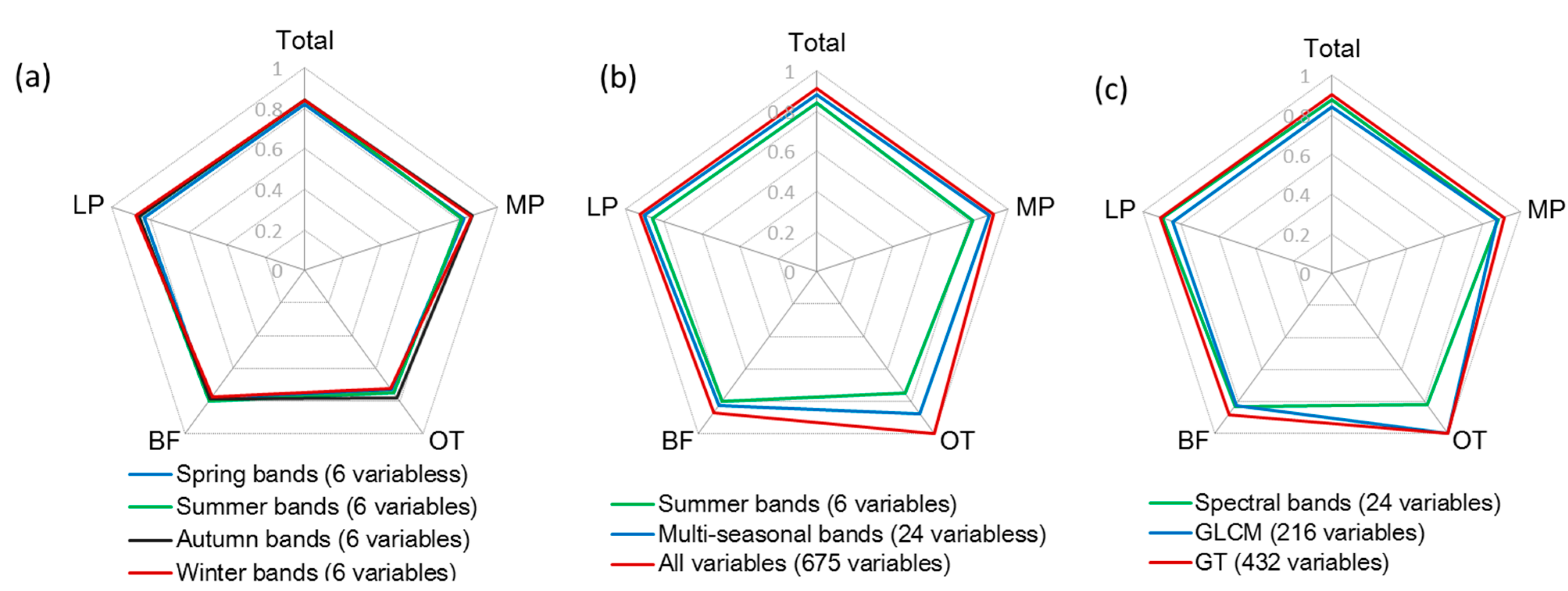
3.1. Performance of Random Forests Classifier

The 675 input variables generated by the multi-seasonal spectral data, two textural measures and topographic data, were used in RF classification to discriminate LP from the other forest types. The accuracy of the RF classifier for all forest types is 91.0%, with a Kappa coefficient of 0.834 (The mtry and ntree of the RF classifier were assigned to 15 and 1000, respectively). To assess the effect of input parameters (mtry and ntree) on classification accuracy, numerous RF classifiers were created for various mtry and ntree. As shown in Figure 3, when mtry is greater than 5, its effect on the overall accuracy of RF classifier is very limited. On the other hand, the overall accuracy increased with an increasing ntree; but this increasing trend is rather weak after 100 trees were grown.

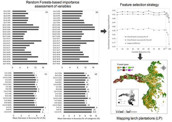
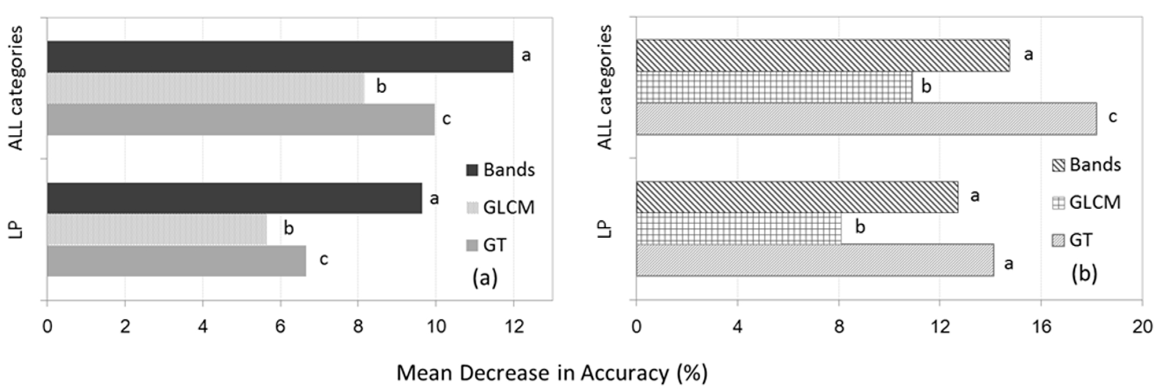
3.2. Importance Measure of Variables

The two textual measures were employed in RF classification directly together with the multi-seasonal spectral data. The result indicates that the classification accuracy difference derived from separate season variables was very minor (Figure 4a). Furthermore, Figure 4b shows the accuracy of RF classifiers using summer bands (main growing season), multi-seasonal bands and all variables, respectively. Comparing the accuracy of RF classifier with summer bands, the inclusion of the extra three season spectral bands produced an increased accuracy of 4.06% for all categories and 3.06% for LP (an increasing Kappa coefficient of 10.19), respectively. Furthermore, adding textural variables to RF model of multi-season spectral bands increases an accuracy of 2.92% for all categories and 1.86% for LP (an increasing kappa coefficient of 3.02), respectively. When the three classes of subsets (spectral bands, GLCM and GT features) were considered in isolation, the subsets of GT features produced the highest accuracy of 90.33% and 91.15% for all categories and for LP, respectively, with a Kappa coefficient of 0.817; the importance of spectral variables and GLCM variables are relatively lower (Figure 4c).
Figure 3. Effect of number of trees and number of random split variables (mtry) on the overall accuracy.
Remotesensing 07 01702 g003
The importance of the three types of variables determined by the RF classifier is shown in Figure 5. It is clear that the importance of multi-seasonal spectral bands was greater than the variables of GLCM and GT (p < 0.05, Figure 5a). Nevertheless, if the most ten effective variables of each subsets were considered, multi-seasonal spectral bands as well as GT measures produced more important variables for the RF classifier (p < 0.05, Figure 5b). The textural variables derived from GLCM measures resulted in consistently less accurate classifications than spectral bands and GT variables (p < 0.05).
The importance of each variable regarding spectral bands, seasons, textural measures and window sizes was assessed in the same way (Figure 6). Figure 6a lists the efficiency of multi-seasonal spectral bands for LP. Several spectral bands appeared to be much more important in summer, autumn and winter than for the rest of the spectral bands, although these important spectral bands varied in different seasons. The bands located in green (OLI3) and red (OLI4) of summer and autumn and those located in shortwave infrared (OLI7) in winter had more predictive power. The difference in importance of spring bands was relatively small. As can be seen, the pattern of important variables for all categories were roughly similar as that for LP, and the most important variables appeared in shortwave infrared-band of winter, red- and green-band of summer and green-band of autumn (Figure 6b).
Figure 4. (a) Spider charts representing the user’s accuracies of RF classifier for the separate season variables; (b) the increase variables; (c) the three separate subsets of variables. The figure includes four forest types: LP, Larix principis-rupprechtii plantations; MP, Pinus sylvestris var. mongolica plantations; BF, Betula platyphylla secondary forests; OT, the other forest types. The tree species of OT are Picea asperata, Pinus tabulaeformis and hardwood deciduous trees. Due to their very low proportion (ca. 2%) of forest types in SFC, they are merged as one class in these figures.
Remotesensing 07 01702 g004
Figure 5. (a) the importance of three types of variables determined by the RF model; (b) the importance of the most ten effective variables determined by the RF model. Bands refer to multispectral bands; GLCM and GT refer to GLCM variables and GT variables, respectively. Topographical variables (altitude, slope and aspect) were not listed due to their relatively low importance. All of the listed results were averaged by the importance of corresponding bands. One-way ANOVA test was applied to compare the importance among the three subsets of input variables. The importance values (bars) with the different letters indicate significant difference (p < 0.05).
Remotesensing 07 01702 g005
Figure 6. Variable importance of the multi-seasonal spectral bands and texture functions. (a) Variable importance of multi-seasonal spectral bands for LP and (b) all categories; (c) variable importance of textural functions and window sizes for LP and (d) all categories. OLI refer to multispectral bands; CON., ENT. and SM. refer to contrast, entropy and second moment, respectively (GLCM textures); VAR., MAD. and PC. refer to variogram, madogram and pseudo-cross variogram, respectively (geostatistical textures). Each value of the multi-seasonal spectral bands repents a single band importance (a,b). The other listed results were averaged importance by corresponding textural measures. One-way ANOVA test was applied to compare the importance of various subsets of input textural variables. The importance values (bars) with the different letters indicate significant difference (p < 0.05).
Remotesensing 07 01702 g006
Various textural measures and window sizes also affected classification accuracy. Figure 6c,d show the importance of textual variables calculated by GLCM and GT measures. In general terms, it was clear from these figures that the importance of bivariate variables derived from PC was greater than that of other univariate variables for LP (p < 0.05). The difference of importance among five kinds of univariate variables with the three window sizes was not significant for both LP and all categories. For bivariate variables, the most relevant window size was 5 × 5 pixels of PC for LP (p < 0.05); however, the effect of window sizes on variable importance was not significant for all categories (p > 0.05, Figure 6d).

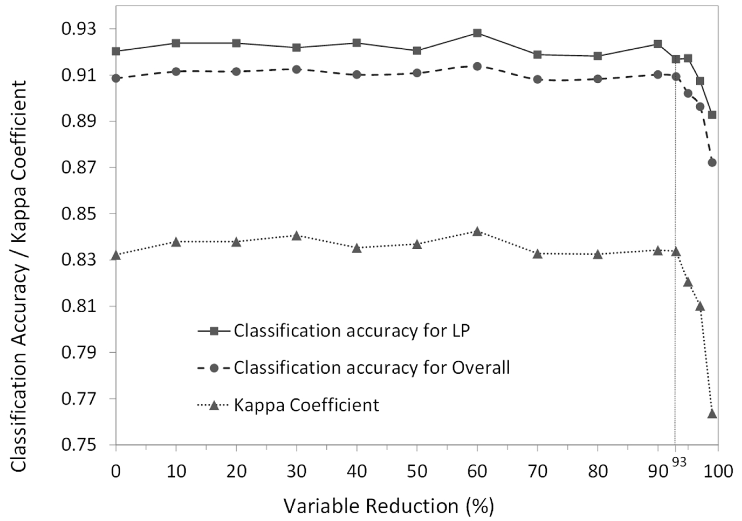
3.3. Mapping LP by Feature Selection of Random Forests

Based on variable importance described in Section 3.2, we attempt to select the most important variables for a RF classifier with little decrease in classification accuracy. Figure 7 illustrates the changes in accuracy and Kappa coefficient for RF models in which the least informative variables were removed gradually. As shown from this figure, the Kappa coefficient and classification accuracy of all categories and LP experienced similar trend, and a well-marked turning point was found (93%). The results shows that the accuracy fluctuated with no significant trend before the turning point (p > 0.05); however, after this turning point, a dramatic decrease in classification accuracy could be observed (R2 = 0.78, p < 0.05).
Figure 7. The effect of variable reduction on classification accuracies.
Remotesensing 07 01702 g007
Based on FS of the RF model, a subset of the most informative variables (47 variables) was applied to a RF model to mapping distribution of LP in SFC (mtry and ntree were assigned to 3 and 200, respectively). The confusion matrix (Table 2) shows that the classification accuracy was similar to the accuracy of RF classifier based on the overall variables (675 variables). The user’s accuracy was 91.9% for LP, which was higher than the other main forest types (Betula platyphylla secondary forests and Pinus sylvestris var. mongolica plantations). Comparing with the user’s accuracy of LP, its producer’s accuracy is marginally higher (94.8% vs. 91.9%). The overall accuracy is 90.7% with a Kappa coefficient of 0.829. Finally, this classifier was applied to produce the LP distribution of SFC. The mapping results were shown in Figure 8. LP had the widest distribution in SFC (47,176 ha, 62.0% of the total forest area), followed by BF (21,094 ha, 27.7% of the total forest area) and MP (7642 ha, 10.0% of the total forest area). The pixels classified represented over 99% of SFC forest area for just these three categories. Less than 1% pixels were classified as AP, PP and HDF (162 ha, 0.2% of the total forest area).
Table 2. Confusion matrix of the RF classifier for the 6 forest types using validation samples. The total accuracy was the percentage of correct-classified samples in total testing samples. LP, Larix principis-rupprechtii plantations; MP, Pinus sylvestris var. mongolica plantations; BF, Betula platyphylla secondary forests; AP, Picea asperata plantations; PP, Pinus tabulaeformis plantations; HDF, hardwood deciduous secondary forests.
Reference DataClassify as
BFHDFLPMPPPAPTotalProd. Acc.
BF7810945008800.888
HDF2302000250
LP8001671110017620.948
MP1027233002610.893
PP00224080.500
AP1022507350.200
total88601818256472971
User’s acc.0.88100.9190.910110.907
Figure 8. Forest types map of SFC using a RF classifier. LP: Larix principis-rupprechtii plantations; MP: Pinus sylvestris var. mongolica plantations; BF: Betula platyphylla secondary forests; AP: Picea asperata plantations; PP: Pinus tabulaeformis plantations; HDF: Hardwood deciduous secondary forests. LP area is 47,176 ha, representing 62.0% of the total forest area; BF area is 21,094 ha, representing 27.7% of the total forest area; MP area is 7642 ha, representing 10.0% of the total forest area; the area of other three forest types area is 162 ha, representing 0.2% of the total forest area.
Remotesensing 07 01702 g008

4. Discussion

4.1. Importance of Input Variables

The 24 multi-seasonal spectral bands improve the classification accuracy substantially, suggesting these original variables carry lots of information about multi-temporal characteristics of different forest types. For spring, summer and autumn, bands at visible wavelengths showed higher importance; however, the near-infrared band importance, which is a key band for vegetation discrimination, is relatively weak. The previous study reported the high efficiency of the near-infrared band in land cover classification [17,32], because it can differentiate vegetation from the other land cover types. The object of our study is forested area (other land cover is excluded), which may be a main reason causing the low importance of near-infrared band in classification. Although the importance of the mono-seasonal near-infrared band is low, its multi-seasonal variability (textural variables calculated by PC) showed a significant importance (Section 4.2). Furthermore, shortwave infrared (OLI7) in winter is the most important of the all multi-seasonal spectral bands. The difference of water content in the canopy and soil among the main forest types may help to explain the high effectiveness of shortwave infrared [45].
The effect of window sizes on textural variable importance differed between univariate texture and bivariate texture. For univariate textural variables, the effect of window sizes on variable importance was not significant; for bivariate textural variables, however, smaller window size outperformed significantly the larger ones (for LP). Generally, larger windows sizes may provide a more accurate representation for homogeneous area [17]. In this study, the bivariate texture tended to describe temporary correlation between the same bands for coupled seasons (multi-seasonal PCs). The partial temporary variability is probably ignored in a large window, whereas a smaller window size may be more representative. Therefore, a small window size should be suggested to obtain a more accurate representation for bivariate textural measures.

4.2. Feature Selection of the most Important Variables

The classification results, which were derived from the subset of the 47 informative variables, suggest that RF-based FS is a reliable approach for reducing redundant variables and improving the classifier efficiency. The subset of the “best” variables included 7 spectral bands, 19 multi-seasonal PCs and 21 multi-band PCs. Although topographic variables were not ranked in this subset, they were high on the list of variable importance; none of univariate textural variables calculated by the two GT (variogram and madogram) and the three GLCM functions (contrast, entropy and second moment) were selected. Previous studies have also reported the good performance of PC for land cover classifications [17,32,37]. Synthetically, these results imply that PC textural measures may have more extensive potential for use in remote sensing-based mapping.
In the subset of the “best” variables, the variables derived from PC textural measures have the greatest influence on class-separability, followed by spectral bands. The most important textural variable was the PC textural variable calculated between the blue and green visible bands of autumn, and that calculated between summer and autumn near-infrared was the most important multi-seasonal textural variables. The near-infrared band was also the most frequent variable appearing in the subset of multi-seasonal textural variables (9 times), although the importance of mono-seasonal near-infrared band is relatively low. Since the near-infrared band is very sensitive to green biomass of forests [33,46], it can cause greater inter-class discriminations with temporal variability in different forest categories. Furthermore, in order to enhance the separability of LP, a time series data set throughout growing cycle of LP was highlighted in this study. We found that the summer variables are the most informative, followed by autumn and winter. The textural variables derived from summer and winter were also the most frequent multi-seasonal PC, probably because of characteristic phenology of forests in SFC, which mainly consisted of LP (deciduous and coniferous forest), MP (evergreen-coniferous forest) and BF (deciduous broad-leaved forest). The variability between growing peak season and non-growing season can maximize the class-separability with a remarkably seasonal behavior [47,48].

4.3. The Accuracy and Uncertainty of Random Forests Classification

RF classifiers derived from the different parameters (mtry and ntree) showed minor differences in classification accuracies when certain value ranges were assigned (mtry was greater than 5 and ntree was greater than 100). It provided highly reliable accuracies for forest type classification [43,49]. The mapping result indicates that LP and MP mainly appeared in the western part and northern part of SFC, while BF was distributed in the eastern and southern part of SFC. This spatial pattern was related to topography of SFC. LP and MP were probably planted in a relatively flat area, whereas natural forest (BF) distributed in a rugged terrain (Figure 8).
Although an encouraging classification result was obtained, the uncertainty in RF classifier was observed. There is a discrepancy between the producer’s and user’s accuracy: For LP, the user’s accuracy was lower than producer’s accuracy; in contrast, for the other forest types, user’s accuracy was greater than producer’s accuracy. This difference suggests that the map produced by RF model tended to misclassify other forest types as LP. The similar misclassification of the RF model has been also reported by previous studies, but the reasons for the misclassifications differed [15,26]. For the present study, the misclassification was probably due to unbalanced proportions of ground samples for different forest types (LP samples accounted for over half of the total ground reference dataset), although a RF classifier can handle unbalanced data well [50]. This problem seems to be hardly resolved due to forest spatial patterns of SFC. We suggest that more studies in various areas should be undertaken to examine the applicability of this method.

5. Conclusions

This study aimed to evaluate the performance of the RF classifier for forest classification and map LP in a typical planted forest area. Multi-seasonal spectral bands as well as textual variables extracted from Landsat-8 OLI were used as input to RF models. The results indicate that using a RF model provided reliable classification results, with minor sensitivity when the certain parameters value ranges were assigned. A RF-based importance assessment was employed. These importance measures show spectral bands and bivariate variables strongly influence forest type-separability in SFC, while the importance of univariate variables is weak. On the basis of importance assessment, a FS strategy was applied to produce a subset of the most important variables. This subset consisted of spectral bands and PC variables. The most effective variable was the PC texture calculated between the blue and green visible bands of autumn. PC texture derived from summer and winter was the most frequent multi-seasonal PC, highlighting that this variability between peak growing season and non-growing season can effectively enhance the forest class-separability. A RF classifier created with the subset of the most important 47 variables produced 91.9% accuracy for LP and 90.7% accuracy for overall forest types, with a Kappa coefficient of 0.829. It should be noted that this classification accuracy was approximately equal to the classification accuracy produced by the RF with all the 675 variables. The main uncertainty of this study, however, would be a tendency of misclassification LP caused by unbalanced proportions of ground samples. The study provides a reference of predictive variables selection of remote sensing and an insight into approaches for mapping plantation forests with phenological behaviors at a regional scale.

Acknowledgments

This research was supported by the National Basic Research Program of China (973 Program, No. 2012CB416906) and China Postdoctoral Science Foundation (No. 2014M561265). We thank Shun Cheng of the Saihanba Forestry Center for providing the ground-truth data.

Author Contributions

Jiaojun Zhu and Tian Gao conceived and designed the experiments; Shangrong Wu, Guiduo Shang and Liyan Huang performed the experiments; Tian Gao and Xiao Zheng analyzed the data; Tian Gao wrote the paper.

Conflicts of Interest

The authors declare no conflict of interest.

References

  1. Mason, W.L.; Zhu, J.J. Silviculture of planted forests managed for multi-functional objectives: Lessons from Chinese and British experiences. In Challenges and Opportunities for the World’s Forests in the 21st Century; Fenning, T., Ed.; Springer: Berlin, Germany, 2014; pp. 39–50. [Google Scholar]
  2. Chinese Ministry of Forestry. Forest Resource Statistics of China; Department of Forest Resource and Management, Chinese Ministry of Forestry: Beijing, China, 2014. (In Chinese) [Google Scholar]
  3. Wang, C.; Ouyang, H.; Shao, B.; Tian, Y.; Zhao, J.; Xu, H. Soil carbon changes following afforestation with Olga Bay Larch (Larix olgensis Henry) in Northeastern China. J. Integr. Plant Biol. 2006, 48, 503–512. [Google Scholar] [CrossRef]
  4. Zhu, J.J.; Yang, K.; Yan, Q.; Liu, Z.; Yu, L.; Wang, H. Feasibility of implementing thinning in even-aged Larix olgensis plantations to develop uneven-aged larch-broadleaved mixed forests. J. For. Res. 2010, 15, 71–80. [Google Scholar] [CrossRef]
  5. Yan, Q.; Zhu, J.J.; Gang, Q. Comparison of spatial patterns of soil seed banks between larch plantations and adjacent secondary forests in Northeast China: Implication for spatial distribution of larch plantations. Trees 2013, 27, 1747–1754. [Google Scholar] [CrossRef]
  6. Yang, K.; Zhu, J.J.; Zhang, M.; Yan, Q.; Sun, O.J. Soil microbial biomass carbon and nitrogen in forest ecosystems of Northeast China: A comparison between natural secondary forest and larch plantation. J. Plant Ecol. 2010, 3, 175–182. [Google Scholar] [CrossRef]
  7. Yang, K.; Shi, W.; Zhu, J.J. The impact of secondary forests conversion into larch plantations on soil chemical and microbiological properties. Plant Soil 2013, 368, 535–546. [Google Scholar] [CrossRef]
  8. Engler, R.; Waser, L.T.; Zimmermann, N.E.; Schaub, M.; Berdos, S.; Ginzler, C.; Psomas, A. Combining ensemble modeling and remote sensing for mapping individual tree species at high spatial resolution. For. Ecol. Manag. 2013, 310, 64–73. [Google Scholar] [CrossRef]
  9. Alkemade, R.; Burkhard, B.; Crossman, N.D.; Nedkov, S.; Petz, K. Quantifying ecosystem services and indicators for science, policy and practice. Ecol. Indic. A 2014, 37, 161–162. [Google Scholar] [CrossRef]
  10. Bijalwan, A.; Swamy, S.L.; Sharma, C.; Sharma, N.; Tiwari, A.K. Land-use, biomass and carbon estimation in dry tropical forest of Chhattisgarh region in India using satellite remote sensing and GIS. J. For. Res. 2010, 21, 161–170. [Google Scholar] [CrossRef]
  11. Gao, T.; Xu, B.; Yang, X.; Jin, Y.; Ma, H.; Li, J.; Yu, H. Using MODIS time series data to estimate aboveground biomass and its spatio-temporal variation in Inner Mongolia’s grassland between 2001 and 2011. Int. J. Remote Sens. 2013, 34, 7796–7810. [Google Scholar] [CrossRef]
  12. Li, J.; Yang, X.; Jin, Y.; Yang, Z.; Huang, W.; Zhao, L.; Gao, T.; Yu, H.; Ma, H.; Qin, Z.; et al. Monitoring and analysis of grassland desertification dynamics using Landsat images in Ningxia, China. Remote Sens. Environ. 2013, 138, 19–26. [Google Scholar] [CrossRef]
  13. Folega, F.; Zhang, C.; Zhao, X.; Wala, K.; Batawila, K.; Huang, H.; Dourma, M.; Akpagana, K. Satellite monitoring of land-use and land-cover changes in northern Togo protected areas. J. For. Res. 2014, 25, 385–392. [Google Scholar] [CrossRef]
  14. Zeng, Y.; Schaepman, M.E.; Wu, B.; Clevers, J.G.P.W.; Bregt, A.K. Scaling-based forest structural change detection using an inverted geometric-optical model in the Three Gorges region of China. Remote Sens. Environ. 2008, 112, 4261–4271. [Google Scholar] [CrossRef]
  15. Grinand, C.; Rakotomalala, F.; Gond, V.; Vaudry, R.; Bernoux, M.; Vieilledent, G. Estimating deforestation in tropical humid and dry forests in Madagascar from 2000 to 2010 using multi-date Landsat satellite images and the random forests classifier. Remote Sens. Environ. 2013, 139, 68–80. [Google Scholar] [CrossRef]
  16. Corcoran, J.; Knight, J.; Gallant, A. Influence of multi-source and multi-temporal remotely sensed and ancillary data on the accuracy of random forest classification of wetlands in Northern Minnesota. Remote Sens. 2013, 5, 3212–3238. [Google Scholar] [CrossRef]
  17. Rodriguez-Galiano, V.F.; Chica-Olmo, M.; Abarca-Hernandez, F.; Atkinson, P.M.; Jeganathan, C. Random Forest classification of Mediterranean land cover using multi-seasonal imagery and multi-seasonal texture. Remote Sens. Environ. 2012, 121, 93–107. [Google Scholar] [CrossRef]
  18. Gong, P.; Wang, J.; Yu, L.; Zhao, Y.; Zhao, Y.; Liang, L.; Niu, Z.; Huang, X.; Fu, H.; Liu, S.; et al. Finer resolution observation and monitoring of global land cover: First mapping results with Landsat TM and ETM+ data. Int. J. Remote Sens. 2012, 34, 2607–2654. [Google Scholar] [CrossRef]
  19. Rodriguez-Galiano, V.; Chica-Olmo, M. Land cover change analysis of a Mediterranean area in Spain using different sources of data: Multi-seasonal Landsat images, land surface temperature, digital terrain models and texture. Appl. Geogr. 2012, 35, 208–218. [Google Scholar] [CrossRef]
  20. Gasparri, N.I.; Parmuchi, M.G.; Bono, J.; Karszenbaum, H.; Montenegro, C.L. Assessing multi-temporal Landsat 7 ETM+ images for estimating above-ground biomass in subtropical dry forests of Argentina. J. Arid Environ. 2010, 74, 1262–1270. [Google Scholar] [CrossRef]
  21. Rakwatin, P.; Longépé, N.; Isoguchi, O.; Shimada, M.; Uryu, Y.; Takeuchi, W. Using multiscale texture information from ALOS PALSAR to map tropical forest. Int. J. Remote Sens. 2012, 33, 7727–7746. [Google Scholar] [CrossRef]
  22. Haralick, R.M.; Shanmugam, K.; Dinstein, I. Textural features for image classification. IEEE Trans. Syst. Man Cybern. 1973, 3, 610–621. [Google Scholar] [CrossRef]
  23. Berberoğlu, S.; Akin, A.; Atkinson, P.M.; Curran, P.J. Utilizing image texture to detect land-cover change in Mediterranean coastal wetlands. Int. J. Remote Sens. 2010, 31, 2793–2815. [Google Scholar] [CrossRef]
  24. Sarker, L.R.; Nichol, J.E. Improved forest biomass estimates using ALOS AVNIR-2 texture indices. Remote Sens. Environ. 2011, 115, 968–977. [Google Scholar] [CrossRef]
  25. Bellman, R. Dynamic Programming, 2nd ed.; Dover Publications: Mineola, NY, USA, 2003. [Google Scholar]
  26. Mellor, A.; Haywood, A.; Stone, C.; Jones, S. The performance of random forests in an operational setting for large area sclerophyll forest classification. Remote Sens. 2013, 5, 2838–2856. [Google Scholar] [CrossRef]
  27. Breiman, L. Random forests. Mach. Learn. 2001, 45, 5–32. [Google Scholar] [CrossRef]
  28. Watts, J.D.; Lawrence, R.L.; Miller, P.R.; Montagne, C. Monitoring of cropland practices for carbon sequestration purposes in north central Montana by Landsat remote sensing. Remote Sens. Environ. 2009, 113, 1843–1852. [Google Scholar] [CrossRef]
  29. Gleason, C.J.; Jungho, I. Forest biomass estimation from airborne LiDAR data using machine learning approaches. Remote Sens. Environ. 2012, 125, 80–91. [Google Scholar] [CrossRef]
  30. Lawrence, R.L.; Wood, S.D.; Sheley, R.L. Mapping invasive plants using hyperspectral imagery and Breiman Cutler classifications (random Forest). Remote Sens. Environ. 2006, 100, 356–362. [Google Scholar] [CrossRef]
  31. Stumpf, A.; Kerle, N. Object-oriented mapping of landslides using Random Forests. Remote Sens. Environ. 2011, 115, 2564–2577. [Google Scholar] [CrossRef]
  32. Fan, H. Land-cover mapping in the Nujiang Grand Canyon: Integrating spectral, textural, and topographic data in a random forest classifier. Int. J. Remote Sens. 2013, 34, 7545–7567. [Google Scholar] [CrossRef]
  33. Roy, D.P.; Wulder, M.A.; Loveland, T.R.; Woodcock, C.E.; Allen, R.G.; Anderson, M.C.; Helder, D.; Irons, J.R.; Johnson, D.M.; Kennedy, R.; et al. Landsat-8: Science and product vision for terrestrial global change research. Remote Sens. Environ. 2014, 145, 154–172. [Google Scholar] [CrossRef]
  34. Congalton, R.G.; Green, K. Assessing the Accuracy of Remotely Sensed Data: Principles and Practices, 2nd ed.; CRC Press: Boca Raton, FL, USA, 2009. [Google Scholar]
  35. Dye, M.; Mutanga, O.; Ismail, R. Detecting the severity of woodwasp, Sirex noctilio, infestation in a pine plantation in KwaZulu-Natal, South Africa, using texture measures calculated from high spatial resolution imagery. Afr. Entomol. 2008, 16, 263–275. [Google Scholar] [CrossRef]
  36. Chica-Olmo, M.; Abarca-Hernández, F. Computing geostatistical image texture for remotely sensed data classification. Comput. Geosci. 2000, 26, 373–383. [Google Scholar] [CrossRef]
  37. Li, P.; Cheng, T.; Guo, J. Multivariate image texture by multivariate variogram for multispectral image classification. Photogramm. Eng. Remote Sens. 2009, 75, 147–157. [Google Scholar] [CrossRef]
  38. Atkinson, P.M.; Lewis, P. Geostatistical classification for remote sensing: An introduction. Comput. Geosci. 2000, 26, 361–371. [Google Scholar] [CrossRef]
  39. Coburn, C.A.; Roberts, A.C.B. A multiscale texture analysis procedure for improved forest stand classification. Int. J. Remote Sens. 2004, 25, 4287–4308. [Google Scholar] [CrossRef]
  40. Pino-Mejías, R.; Cubiles-De-La-Vega, M.D.; Anaya-Romero, M.; Pascual-Acosta, A.; Jordán-López, A.; Bellinfante-Crocci, N. Predicting the potential habitat of oaks with data mining models and the R system. Environ. Model. Softw. 2010, 25, 826–836. [Google Scholar] [CrossRef]
  41. Chan, J.C.; Paelinckx, D. Evaluation of random forest and adaboost tree-based ensemble classification and spectral band selection for ecotope mapping using airborne hyperspectral imagery. Remote Sens. Environ. 2008, 112, 2999–3011. [Google Scholar] [CrossRef]
  42. Rodriguez-Galiano, V.F.; Ghimire, B.; Rogan, J.; Chica-Olmo, M.; Rigol-Sanchez, J.P. An assessment of the effectiveness of a random forest classifier for land-cover classification. ISPRS J. Photogramm. Remote Sens. 2012, 67, 93–104. [Google Scholar] [CrossRef]
  43. Immitzer, M.; Atzberger, C.; Koukal, T. Tree Species Classification with random forest using very high spatial resolution 8-band worldview-2 satellite data. Remote Sens. 2012, 4, 2661–2693. [Google Scholar] [CrossRef]
  44. Cutler, D.R.; Edwards, T.C.; Beard, K.H.; Cutler, A.; Hess, K.T.; Gibson, J.; Lawler, J.J. Random forests for classification in ecology. Ecology 2007, 88, 2783–2792. [Google Scholar] [CrossRef] [PubMed]
  45. Hunt, E.R., Jr.; Li, L.; Yilmaz, M.T.; Jackson, T.J. Comparison of vegetation water contents derived from shortwave-infrared and passive-microwave sensors over central Iowa. Remote Sens. Environ. 2011, 115, 2376–2383. [Google Scholar] [CrossRef]
  46. Plummer, S.E. Exploring the relationships between leaf nitrogen content, biomass and the near-infrared/red reflectance ratio. Int. J. Remote Sens. 1988, 9, 177–183. [Google Scholar] [CrossRef]
  47. Ghioca-Robrecht, D.; Johnston, C.; Tulbure, M. Assessing the use of multiseason QuickBird imagery for mapping invasive species in a Lake Erie coastal Marsh. Wetlands 2008, 28, 1028–1039. [Google Scholar] [CrossRef]
  48. Helmer, E.H.; Ruzycki, T.S.; Benner, J.; Voggesser, S.M.; Scobie, B.P.; Park, C.; Fanning, D.W.; Ramnarine, S. Detailed maps of tropical forest types are within reach: Forest tree communities for Trinidad and Tobago mapped with multiseason Landsat and multiseason fine-resolution imagery. For. Ecol. Manag. 2012, 279, 147–166. [Google Scholar] [CrossRef]
  49. Li, C.; Wang, J.; Hu, L.; Yu, L.; Clinton, N.; Huang, H.; Yang, J.; Gong, P. A circa 2010 thirty meter resolution forest map for China. Remote Sens. 2014, 6, 5325–5343. [Google Scholar] [CrossRef]
  50. Pal, M. Random forest classifier for remote sensing classification. Int. J. Remote Sens. 2005, 26, 217–222. [Google Scholar] [CrossRef]

