An Algorithm for Gross Primary Production (GPP) and Net Ecosystem Production (NEP) Estimations in the Midstream of the Heihe River Basin, China

Abstract

An accurate estimation of carbon fluxes is very important in carbon cycle studies. A remote sensing based gross primary production (GPP) and net ecosystem production (NEP) algorithm, RS-CFLUX, was presented in this work. The algorithm was calibrated with Markov Chain Monte Carlo (MCMC) method at Daman superstation and Zhangye wetland station in the midstream of the Heihe River Basin. Results indicated that both of the stations present high GPP (1442.04 g C/m²/year at Daman superstation and 928.89 g C/m²/year at Zhangye wetland station) and NEP (409.38 g C/m²/year at Daman superstation and 422.60 g C/m²/year at Zhangye wetland station). The RS-CFLUX model can correctly simulate the seasonal dynamics and quantities of carbon fluxes at both stations, using photosynthetically active radiation (PAR), land surface temperature (LST), normalized difference water index (NDWI) and enhanced vegetation index (EVI) as input. RS-CFLUX model were sensitive to maximum light use efficiency, respiration at reference temperature, activation energy parameter of respiration.

1. Introduction

Vegetation can be affected by climate change through the energy and mass exchange between vegetation and atmosphere [1,2,3]. Carbon flux is a mass exchange that is related to global warming [4,5]. Accurate estimation of carbon flux plays an important role in carbon cycle study. Generally, two types of methods can be used to estimate carbon flux: observing and modeling. Observing instrument (such as Eddy covariance) can measure the continuous exchange of carbon flux at a specific site with an area of several square kilometers. However, model can efficiently estimate carbon flux at regional scale.

Remote sensing is an important source of data for simulating carbon flux. In recent years, many remote sensing based carbon flux models were developed, such as Glo-PEM [6], C-Fix [7,8], VPM [9], MODIS GPP/NPP algorithm [10], and DCFM [11]. All of these models use air temperature as an input. At many observation stations, the air temperature is observed above the canopy, and is different from the canopy temperature [12,13], which actually controls photosynthesis and respiration of vegetation. During the growing season, the land surface temperature (LST) within a high vegetation coverage area is dominated by the canopy temperature. With the development of remote sensing, more and more thermal infrared data is available to estimate LST. MODIS provide thermal infrared image twice every day with spatial resolution of 1 km. Landsat series data provide thermal infrared image every 16 days with spatial resolution of 100 m. These datasets can be used to retrieve continuous LST, which can force carbon flux model. Thus, LST could be used as inputs in remote sensing based carbon flux estimation.

The Heihe River Basin, which is located in Northwest China, is the second largest inland river basin in the country [14]. In the midstream of the Heihe River Basin, yearly rainfall is less than 100 mm. Most of the area is Gobi Desert, which has little carbon flux. The largest vegetated area in the midstream of the Heihe River Basin is irrigated cropland. Another well-vegetated area is wetland because of abundant water supply from ground water and river water. Irrigated croplands and wetlands are the two ecosystems with the highest production in the midstream of the Heihe River Basin. Carbon fluxes of these two ecosystems contribute the majority of carbon flux in the midstream of the Heihe River Basin. Thus the accurate estimating of carbon fluxes of these two ecosystems is very important to evaluate the regional scale carbon flux of the midstream of the Heihe River Basin.

Hence, the objectives of this study were to (1) analyze the carbon flux characteristics of irrigated croplands and wetlands in midstream of the Heihe River Basin; (2) develop a remote sensing based carbon flux algorithm, RS-CFLUX, to simulate the carbon flux quantity and dynamics at the two ecosystems.

2. Materials and Method

2.1. Data Acquisition

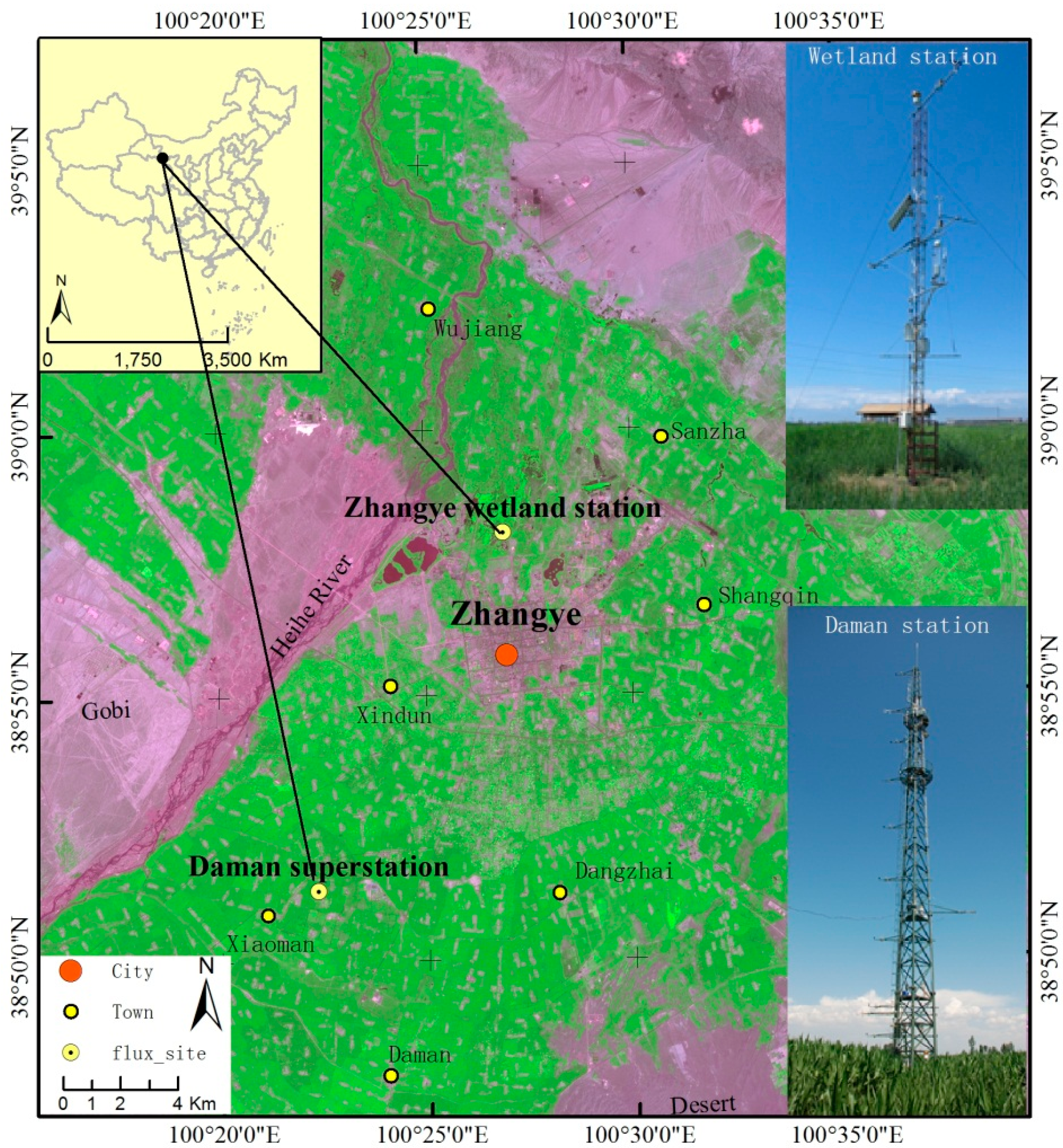
2.1.1. Observation Stations

Eddy covariance (EC) and automatic meteorological station (AMS) data in 2013 was collected at Daman superstation and Zhangye wetland station. These two observation stations were established during HiWATER experiment in May of 2012 [15]. Figure 1 shows the location and photos of Daman superstation and Zhangye wetland station.

Figure 1. Location of the Daman superstation and Zhangye wetland station. (The background image is ASTER image, red: 556 nm, green: 807 nm, red: 661 nm).

Figure 1. Location of the Daman superstation and Zhangye wetland station. (The background image is ASTER image, red: 556 nm, green: 807 nm, red: 661 nm).

The observing items and information of Daman superstation and Zhangye wetland station are listed in Table 1. Meteorological data was sampled every minute and was converted to a 30-min average value for comparison with the flux data. Values were deleted if they were beyond the physical range or instrument range [16]. The EC systems at the two stations consist of an open-path infrared gas analyzer and a 3-D sonic anemometer [17,18]. The 3-D wind speed, H₂O concentration and CO₂ concentration data were sampled at a frequency of 10 Hz by a data logger. Half hour fluxes were calculated by post-processing raw 10 Hz data using the EdiRe software. The processing steps include spike detection, lag correction of H₂O/CO₂ relative to the vertical wind component, sonic virtual temperature conversion, planar fit coordinate rotation, the WPL (Webb-Pearman-Leuning) density fluctuation correction and frequency response correction [16].

Half-hourly flux data were excluded if the instrument range was excessive, rainfall occurred or instrument malfunctions occurred. At night (downward short wave radiation < 1 W/m²), half-hourly flux data were excluded if friction velocity (u*) was lower than a specific threshold (0.15 m/s), because of weak turbulent mixing at a low friction velocity. Then, missing values in the fluxes were filled using non-linear functions, which use PAR and air temperature as input. Missing values in the fluxes were not filled when the meteorological measurements were not simultaneously available. The gap-filling data were used only to analyze the seasonal and annual variations in the carbon flux. GPP was the sum of the daytime net ecosystem production (NEP) and ecosystem respiration (ER). The daytime ER was estimated with the Van’t Hoff function which was calibrated using the night-time air temperature and nocturnal NEE. The specific method and formulas in the NEE partitioning can be found in Wang’s paper [19,20].

Table 1. Observing items at the Daman superstation and Zhangye wetland station.

Measurements	Daman Superstation	Zhangye Wetland Station
Location	100.3722° E, 38.8555° N	100.4464° E, 38.9751° N
Elevation	1556.06 m	1460.00 m
Land cover	Maize	Reed
Wind speed	3 m, 5 m, 10 m, 15 m, 20 m, 30 m and 40 m	5 m and 10 m
Wind direction	3 m, 5 m, 10 m, 15 m, 20 m, 30 m and 40 m	10 m
Air temperature, relative humidity	3 m, 5 m, 10 m, 15 m, 20 m, 30 m and 40 m	5 m and 10 m
CO2 concentration	3 m, 5 m, 10 m, 15 m, 20 m, 30 m and 40 m	No measurement
Air pressure	2 m	2 m
Land surface temperature	12 m
PAR	12 m	6 m
Soil heat flux	6 cm	6 cm
Soil temperature	0 cm, 2 cm, 4 cm, 10 cm, 20 cm, 40 cm, 80 cm, 120 cm and 160 cm	0 cm, 2 cm, 4 cm, 10 cm, 20 cm and 40 cm
Soil moisture	2 cm, 4 cm, 10 cm, 20 cm, 40 cm, 80 cm, 120 cm and 160 cm	No measurement
Rainfall	2.5 m	10 m
EC systems	4.5 m	5.2 m

Table 1. Observing items at the Daman superstation and Zhangye wetland station.

Measurements	Daman Superstation	Zhangye Wetland Station
Location	100.3722° E, 38.8555° N	100.4464° E, 38.9751° N
Elevation	1556.06 m	1460.00 m
Land cover	Maize	Reed
Wind speed	3 m, 5 m, 10 m, 15 m, 20 m, 30 m and 40 m	5 m and 10 m
Wind direction	3 m, 5 m, 10 m, 15 m, 20 m, 30 m and 40 m	10 m
Air temperature, relative humidity	3 m, 5 m, 10 m, 15 m, 20 m, 30 m and 40 m	5 m and 10 m
CO2 concentration	3 m, 5 m, 10 m, 15 m, 20 m, 30 m and 40 m	No measurement
Air pressure	2 m	2 m
Land surface temperature	12 m
PAR	12 m	6 m
Soil heat flux	6 cm	6 cm
Soil temperature	0 cm, 2 cm, 4 cm, 10 cm, 20 cm, 40 cm, 80 cm, 120 cm and 160 cm	0 cm, 2 cm, 4 cm, 10 cm, 20 cm and 40 cm
Soil moisture	2 cm, 4 cm, 10 cm, 20 cm, 40 cm, 80 cm, 120 cm and 160 cm	No measurement
Rainfall	2.5 m	10 m
EC systems	4.5 m	5.2 m

2.1.2. Remote Sensing Data

Moderate-resolution imaging spectroradiometer (MODIS) remote sensing data products are frequently used in light use efficiency models. MODIS provides high temporal resolution images of the land surface. The sensor contains 36 bands in the visible (459 nm) to thermal-infrared band (14,385 nm). Vegetation indices and land surface temperature can be retrieved from these bands. Many land surface variables products were estimated and distributed by the Land Processes Distributed Active Archive Centre (LP DAAC), and are widely used in scientific research. In this study, the 8-day land surface reflectance product (MOD09A1) and daily land surface temperature product (MOD11A1) were downloaded from the website of MODIS Land Product Subsets [21,22]. The vegetation indices (EVI and NDWI) were estimated from the MOD09A1. MOD09A1 data were resampled to 1 km spatial resolution. The temporal profiles of the vegetation indices and LST were extracted according to the geographical coordinates of the two stations. The vegetation indices were smoothed using the Savizky-Golay algorithm [23] and were interpolated into daily data.

The formulas for EVI, NDWI and the Savizky-Golay algorithm are as follows:

$$EVI=G\times ({\rho }_{nir}-{\text{ρ}}_{red})/({\rho }_{nir}+(C_1\times {\rho }_{red}-C_2\times {\rho }_{blue})+\mathrm{L})$$

(1)

$$NDWI=\frac{{\rho }_{nir}-{\rho }_{sir}}{{\rho }_{nir}+{\rho }_{sir}}$$

(2)

$$Y_i^{*}=\frac{1}{2m+1}{\displaystyle {\sum }_{j=-m}^{j=m}{C}_j{Y}_{i+j}}$$

(3)

where G is 2.5, C₁ is 6, C₂ is 7.5 and L is 1, ρ_blue, ρ_red, ρ_nir and ρ_sir are the reflectance of the blue (band 4), red (band 1), near infrared (band 2) and shortwave infrared bands (band 6), Y is the original time-series data, Y_i^* is the reconstructed time-series data, C_j is the jth weight of the filter window and 2 m + 1 is the size of the filter window. The window size and order of Savizky-Golay algorithm were set to 13 and 4 based on previous studies [24,25].

2.2. Remote-Sensing-Based Carbon Flux Model

2.2.1. GPP Estimation

The general form of light use efficiency (LUE) approach is as follows,

$$GPP=PAR\times fAPAR\times LU{E}_{\max }\times f(T)\times f(W)$$

(4)

where GPP (g C/m²/day) represents absorbed CO₂, PAR (MJ/m²/day) is photosynthetically active radiation, fAPAR (dimensionless) is the fraction of absorbed PAR by the canopy, and LUE_max (g C/MJ) is the maximum LUE. f(T) (dimensionless) and f(W) (dimensionless) are temperature and water scalars, respectively.

2.2.2. fAPAR

fAPAR is usually retrieved from vegetation indices, such as the normalized difference vegetation index (NDVI) and enhanced vegetation index (EVI). The EVI is an optimized vegetation index developed from the NDVI, and it has a strong seasonal correlation with GPP [26,27]. Recent studies indicated that fAPAR should be partitioned into the fraction of PAR absorbed by chlorophyll and by non-photosynthetically active components. In addition, the EVI equals to the PAR absorbed by chlorophyll according to Xiao’s study [9].

$$fAPAR=EVI$$

(5)

2.2.3. Temperature Scalar

In many LUE models, temperature scalars are calculated using near-surface air temperature, because it is easy to obtain from site-based meteorological measurements. When estimating regional carbon fluxes using LUE models, site-observed near-surface air temperature is interpolated into gridded data, which is spatially and temporally consistent with remote sensing data. This process can lead to uncertainties when estimating the results. In this study, we attempt to use LST as the input for the LUE model, because high temporal and spatial resolution LSTs can be estimated using thermal infrared remote sensing images. The temperature scalar is estimated at each time step, using the equation developed for the Terrestrial Ecosystem Model [28]:

$$f(T)=\frac{(LST-LS{T}_{\min })(LST-LS{T}_{\max })}{(LST-LS{T}_{\min })(LST-LS{T}_{\max })-{(LST-LS{T}_{opt})}^2}$$

(6)

where LST (°C) is the land surface temperature, LST_max (°C), LST_opt (°C) and LST_min (°C) are the maximum, optimum, and minimum land surface temperature for photosynthesis, respectively. f(T) equals 0 when the LST is more than LST_max or less than LST_min.

2.2.4. Water Scalar

Water status f (W) is another important environmental factor that affects the photosynthesis rate. f (W) is usually calculated using different variables in LUE models, such as soil water content in Glo-PEM [6]. These variables are only observed at a few of points in a particular area. The process of converting from point data to spatially gridded data leads to uncertainties in LUE model results. The normalized difference water index (NDWI) is a remote sensing data based index that can reflect the water content of vegetation [29]. Xiao [9] used the NDWI to calculate water scalar of LUE model. We also used this formula to estimate f (W).

$$f(W)=(1+NDWI)/(1+NDW{I}_{max})$$

(7)

where NDWI_max (dimensionless) is maximum NDWI during the peak of the growing season.

2.2.5. NEP Estimation

Net ecosystem production (NEP) is the difference between GPP and ecosystem ER. The Lloyd-Taylor respiration function is widely used in ecosystem respiration calculation [30]. Here, the Lloyd-Taylor respiration function was modified in two ways. First, in order to consider the impact of seasonal changes in biomass on respiration, a × EVI was added to the respiration rate at the reference temperature [11]. Second, air temperature was replaced with LST. The formula is as follows:

$$NEP=GPP-ER=GPP-(Rref+a\times EVI){e^{E0}}^{(\frac{1}{56.02}-\frac{1}{(LST+46.02)})}$$

(8)

where Rref (g C/m²/day) is the respiration rate at the reference temperature, and a (g C/m²/day) is an empirical coefficient. E0 (°C) is the activation energy parameter, which determines sensitivity of the respiration to temperature.

2.3. Model Calibration Method

Remote sensing based carbon flux models usually contain many parameters. When the models are used to simulate carbon flux at a specific site, the parameters should be calibrated. Bayesian theory based parameter estimation method, Markov Chain Monte Carlo (MCMC), is very popular in recent years, because it not only solves the value of parameters but also predicts the posterior probability distribution function of parameters. The posterior probability distribution function can help us to know the characteristics of model parameters and how the parameters will impact on models’ output. The MCMC method contains two repeated steps: a proposal step and a movement step [31,32].

In the proposal step, a newly proposed parameter is generated from the previous accepted parameters with a random walk Δc. Δc is calculated using a random number r between 0 and 1, the parameter range (c_{max −} c_min) and a step length factor s. s equals to 5, according to a previous study [31].

$$c^{i+1}=c^i+\mathrm{\Delta }c=c^i+\frac{(r-0.5)}{s}(c_{\max }-c_{\min })$$

(9)

where cⁱ⁺¹ and cⁱ are the proposed parameter vector and previously accepted parameters vector, respectively.

In the movement step, cⁱ⁺¹ is tested using the Metropolis rule to determine if the parameter should be accepted. The accepted probability (p(cⁱ, cⁱ⁺¹) ) of the proposed parameters is derived from the likelihood function (L(c)) using the parameters accepted previously. The mathematical formula is as follows:

$$L(c)={\displaystyle \prod _{i=1}^m}{\displaystyle \prod _{t=1}^n\frac{1}{\sqrt{2\pi \delta }}}{\mathrm{e}}^{-\frac{{(Cflu{x}_t^o-Cflu{x}_t^s)}^2}{2{\text{δ}}^2}}$$

(10)

$$p(c^i,c^{i+1})=\min \{1,L(c^{i+1})/L(c^i)\}$$

(11)

where Cflux_t^o and Cflux_t^s are the in-situ and RS-CFLUX model predicted carbon flux, respectively. δ is the standard deviation of the data-model difference. m is the number of datasets used in the cost function, and n is the number of observations. Then, the acceptance probability is compared with a uniform random number U [0, 1]. Only when the acceptance probability is greater than U, will cⁱ⁺¹ be accepted.

In this study, five parallel MCMC chains with 50,000 iterations each were run in the calibration process. The first 10,000 iterations of each chain were burn-in iterations and were deleted. The remaining iterations of the parameters were used to generate posterior distributions. G-R diagnostic method [33] was used to evaluate the chain convergence. The MCMC algorithm was programmed in Matlab code.

2.4. Model Accuracy Evaluation

Three indices were used to evaluate the performance of the model. (1) The coefficient of determination (R²), which describes to what extent the variation in the observations can be explained by the models. R² ranges from 0 to 1, where a value near 1 indicates a good performance of the model. (2) The root mean square error (RMSE) represents the sample standard deviation of the differences between the predicted values and observed values. A smaller RSME indicates a better performance of the model. (3) The Nash-Sutcliffe model efficiency coefficient (NSE) is often used to assess the power of a model. The coefficient ranges from −∞ to 1. A NSE close to 1 indicates a better match between the modeled and observed values. The formulas for R², RMSE and NSE are as follows:

$$R^2=1-\frac{{\displaystyle \sum _{t=1}^{t=n}{(M_t-O_t)}^2}}{{\displaystyle \sum _{t=1}^{t=n}{(O_t)}^2}}$$

(12)

$$RMSE=\sqrt{\frac{1}{n}{\displaystyle \sum _{t=1}^{t=n}{(M_t-O_t)}^2}}$$

(13)

$$NSE=1-\frac{{\displaystyle \sum _{t=1}^{t=n}{(O_t-M_t)}^2}}{{\displaystyle \sum _{t=1}^{t=n}{(O_t-\overline{O})}^2}}$$

(14)

where O_t is observed value at time t, M_t is the predicted value at time t, and n is the number of observations. $\overline{O}$ is the mean of the observations.

3. Results

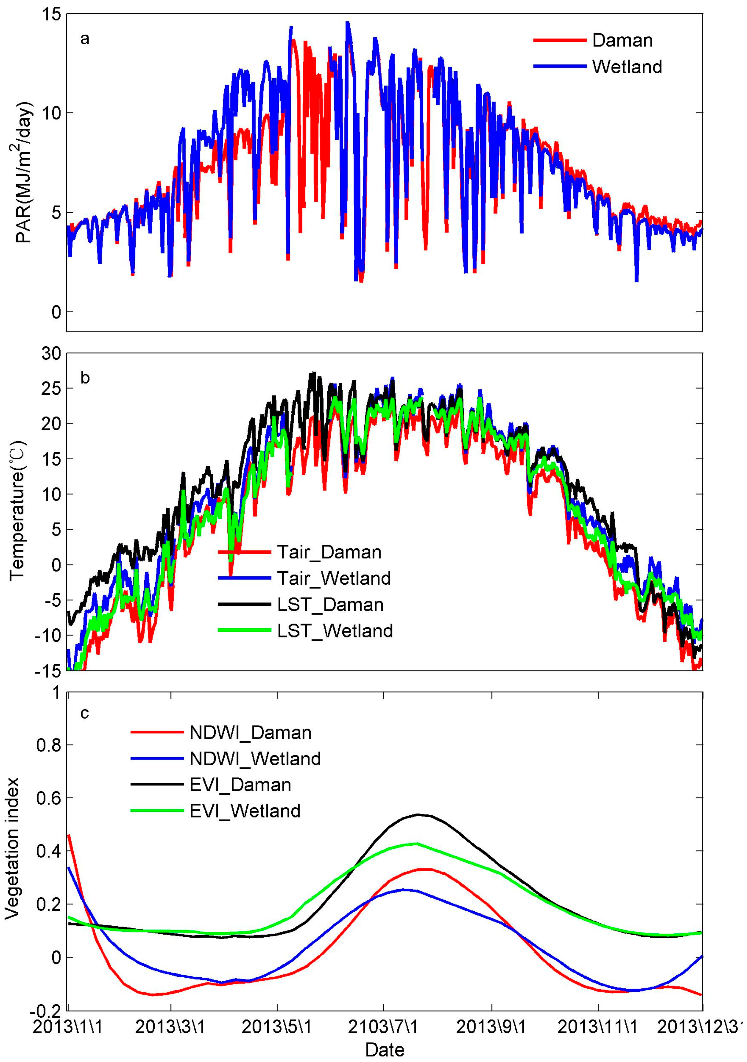
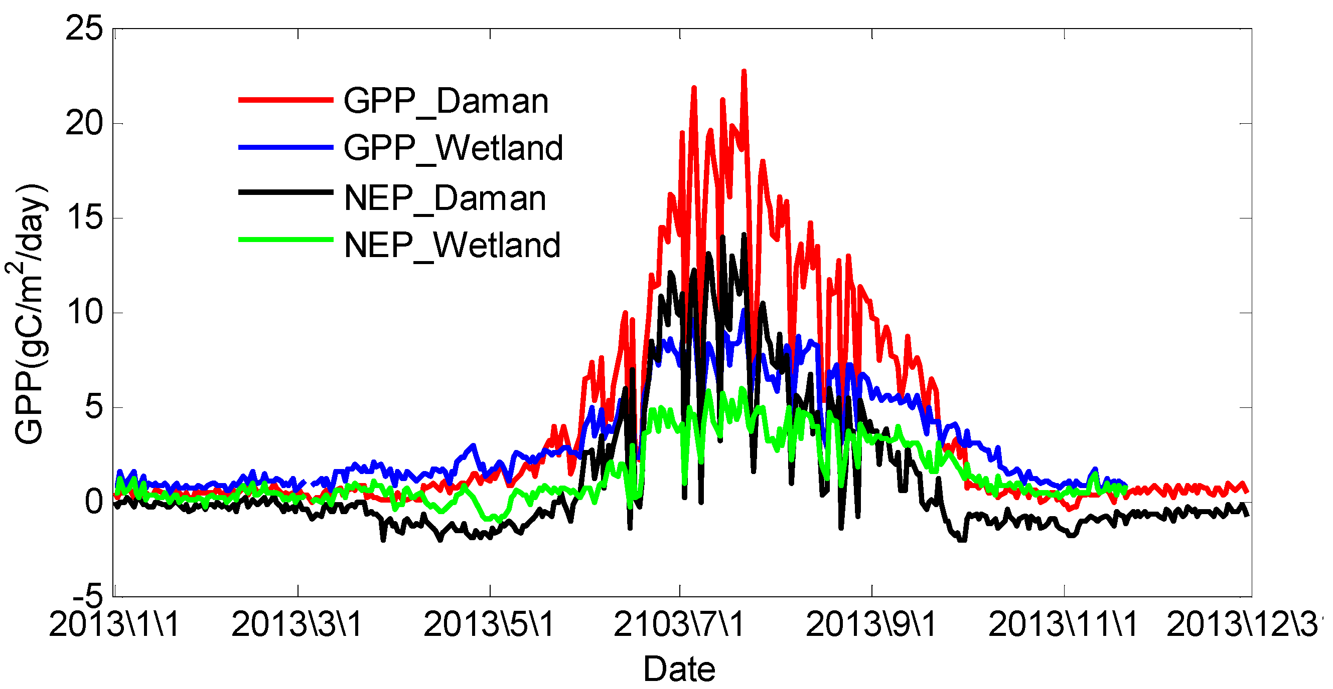
3.1. Seasonal Dynamics of the Carbon Flux and Environmental Factors

The seasonal dynamics of PAR, LST, air temperature, NDWI and EVI are shown in Figure 2.

Figure 2. Seasonal dynamics of the PAR (a), air temperature (Tair), land surface temperature (LST) (b) and vegetation indices (NDWI and EVI) (c) at the Daman superstation and Zhangye wetland station.

Figure 2. Seasonal dynamics of the PAR (a), air temperature (Tair), land surface temperature (LST) (b) and vegetation indices (NDWI and EVI) (c) at the Daman superstation and Zhangye wetland station.

The PAR values observed at the two stations were very consistent in terms of the quantity and seasonal dynamics, except the period from early March to early May (See Figure 2a). At the Zhangye wetland station, the LST was close to the air temperature for entire year. However, at the Daman superstation, the LST was higher than the air temperature. Specifically, the soil surface at Zhangye wetland station remained wet all year, whereas the soil surface was dry for most of the year at the Daman superstation (see Figure 2b). The two stations had the same seasonal trends of vegetation indices (EVI and NDWI). At the Daman superstation, the EVI and NDWI reached their maximum values (0.53 and 0.33, respectively) in late July. At the Zhangye wetland station, the EVI and NDWI reached their maximum values (0.45 and 0.26, respectively) in the middle of July. At the peak of the growing season, the EVI and NDWI were higher at Daman superstation than the Zhangye wetland station, and vice versa at the beginning and end of the growing season. Furthermore, reed has a longer growing season than maize, because EVI of reed start increasing earlier than maize and decrease at the same time (see Figure 2c).

The seasonal dynamics of in-situ GPP and NEP are shown in Figure 3. The GPP and NEP of the Daman superstation (maize) were higher than those of the Zhangye wetland station (reed) during the growing season (see Figure 3), but were lower in the non-growing season. The maximum GPP was 22.64 g C/m²/day at the Daman superstation and 10.06 g C/m²/day at the Zhangye wetland station. The maximum NEP was attained during the peak of the growing season and was 14.02 g C/m²/day at the Daman superstation and 5.90 g C/m²/day at the Zhangye wetland station. The minimum NEP was attained in late April and early October. In 2013, the GPP at the Daman superstation was 1442.04 g C/m²/year, and the GPP at the Zhangye wetland station was 928.89 g C/m²/year (GPP for 20 days in May, 5 days in July, and days from the November 21 to the end of 2013 were missed). The NEP of 2013 is 409.38 g C/m²/year for the Daman superstation and 422.60 g C/m²/year for the Zhangye wetland station. During the non-growing season, carbon was slightly absorbed at the Zhangye wetland station.

Figure 3. Seasonal dynamics of the GPP and NEP at the Daman superstation and Zhangye wetland station.

Figure 3. Seasonal dynamics of the GPP and NEP at the Daman superstation and Zhangye wetland station.

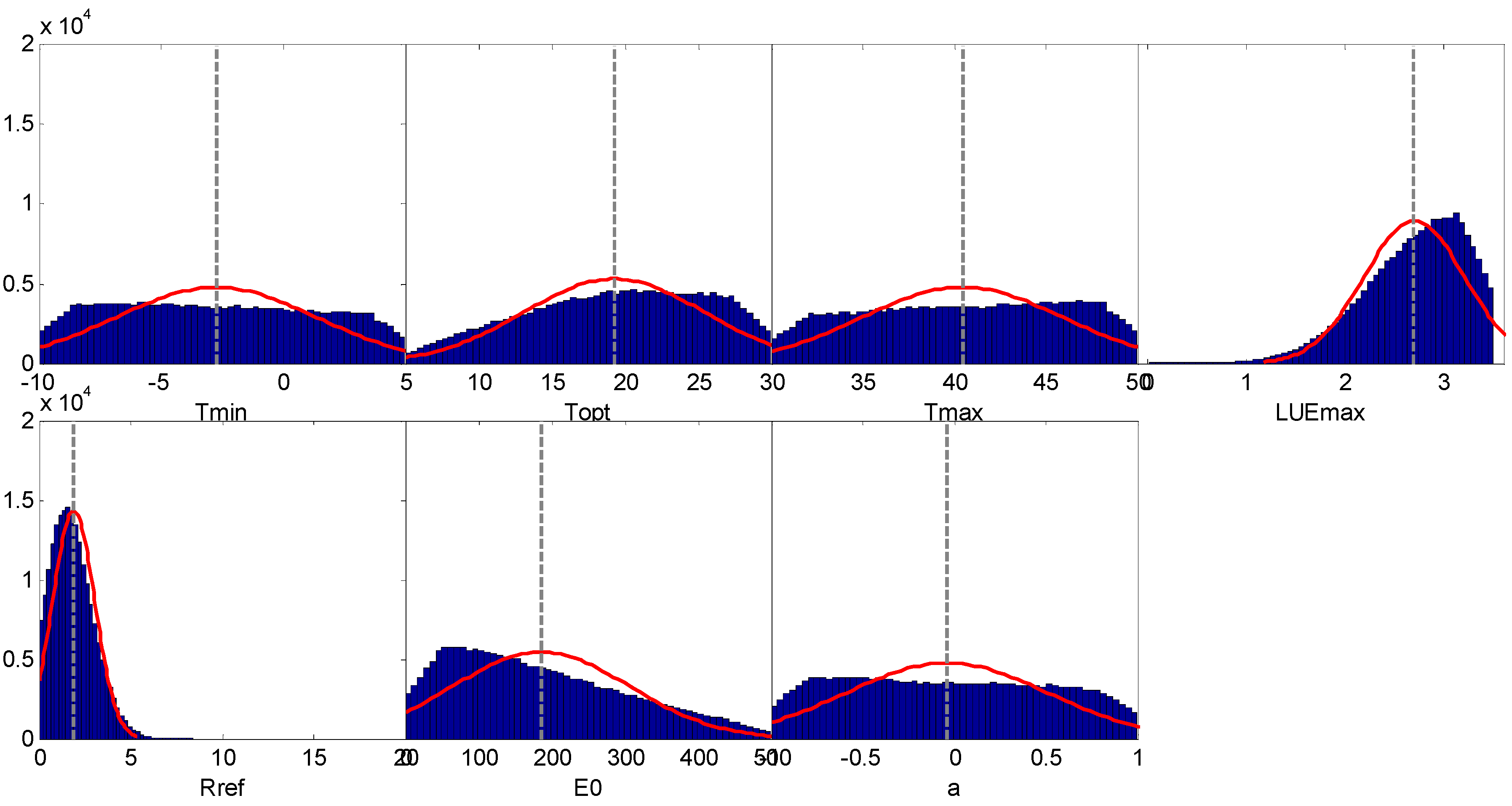
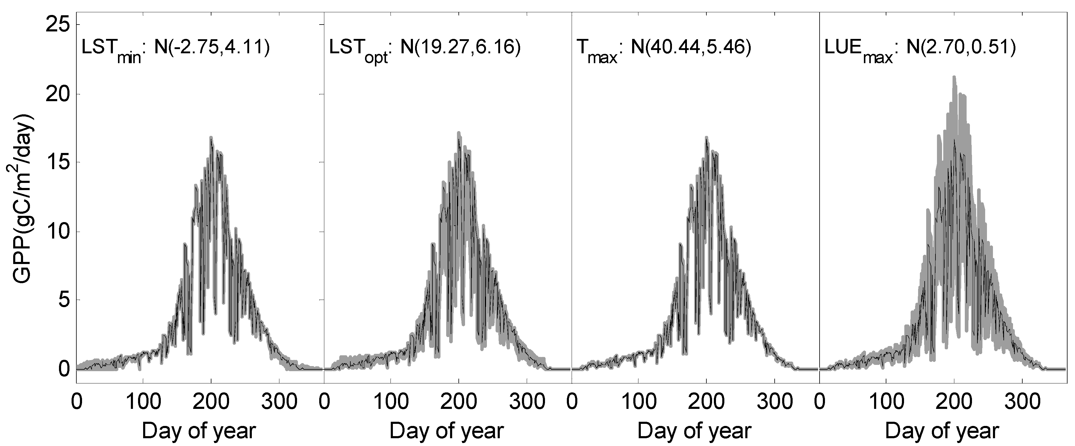
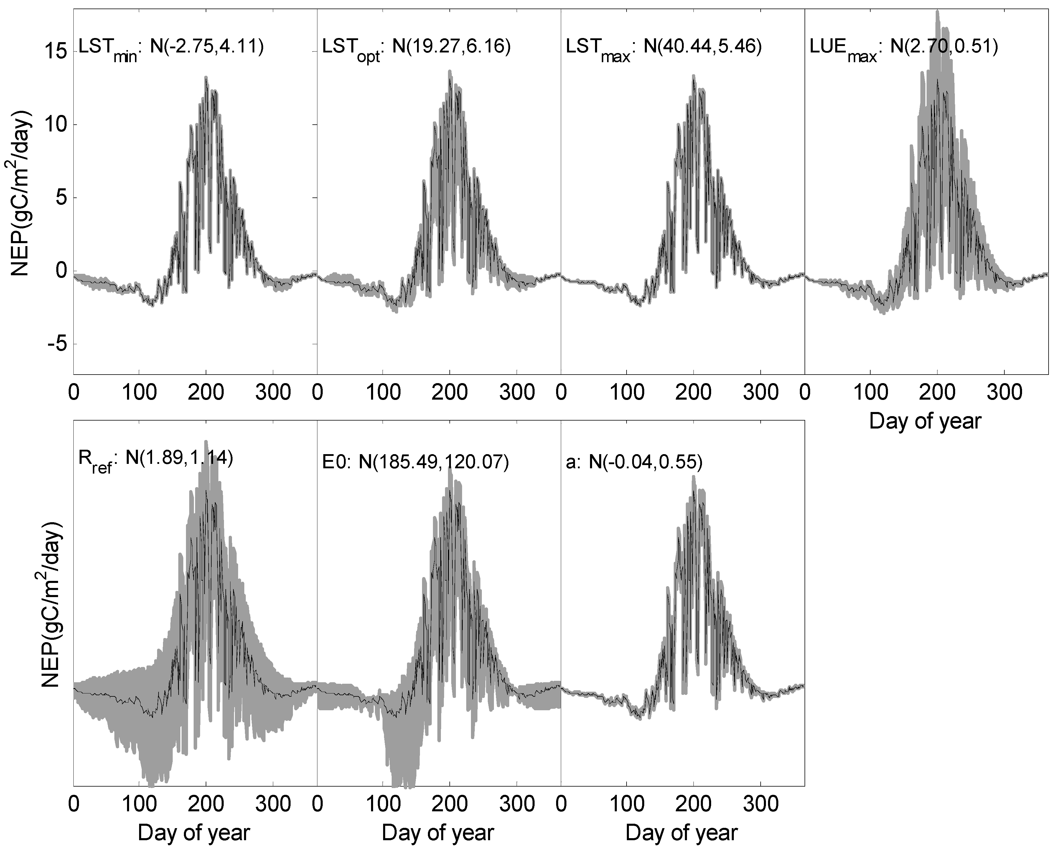
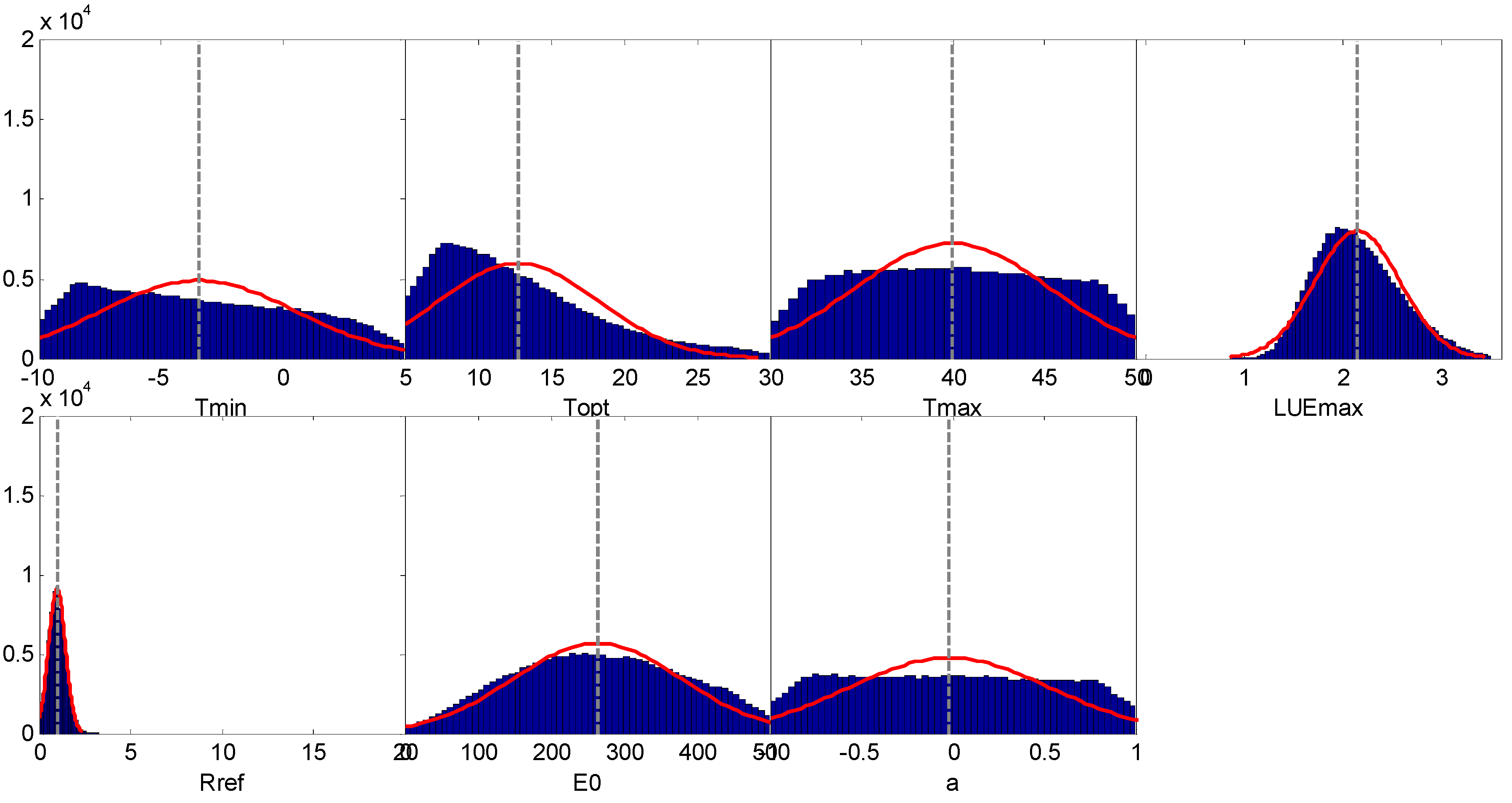
3.2. Calibration of the RS-CFLUX Model at the Two Stations

The prior value and range of the parameters were obtained from the literature or from conventional knowledge. The posterior value and range of the parameters in the RS-CFLUX model were estimated using the MCMC method (see Table 2, Figure 4 and Figure 5). From the posterior distribution of parameters, we found that LUE_max was well constrained at both stations. The value of 2.70 g C/MJ of LUE_max at the Daman superstation was much higher than the value of 2.15 g C/MJ at the Zhangye wetland station. LST_max, LST_opt and LST_min were not well constrained. LST_max and LST_min were very similar at the two stations, but LST_opt was obviously higher for maize than for reed. The range from LST_min to LST_max for maize was smaller than that for reed because the growing season for maize is shorter than for reed. Respiration rate at reference temperature Rref was also well constrained at both stations, but empirical parameter of respiration function E0 and a were not well constrained at either site.

Table 2. Prior distribution (initial value and range) and posterior distribution (mean value and 95% confidence interval) of the parameters of the RS-CFLUX model at the Daman superstation (Daman) and Zhangye wetland station (Wetland).

Parameter	Prior	Posterior (Daman)	Posterior (Wetland)
LSTmin (°C)	−3(−10, 5)	−2.75 (−9.44, 4.35)	−3.47 (−9.54,4.02)
LSTopt (°C)	15(5, 30)	19.27 (7.16, 29.07)	12.78 (5.52,26.30)
LSTmax (°C)	35(30, 50)	40.44 (30.93,49.26)	39.98 (30.94,49.16)
LUEmax (gC/MJ)	2(0, 3.5) [34,35]	2.70 (1.55,3.44)	2.15 (1.42,3.08)
Rref (gC/m2/day)	2(0,20) [11]	1.89 (0.15,4.46)	0.98 (0.17,1.97)
E0 (°C)	200(0,500) [11]	185.49 (13.90,445.41)	263.70 (50.34,471.57)
a (gC/m2/day)	0.8(−1,1) [11]	−0.04 (−0.93,0.91)	−0.01 (−0.92,0.92)

Table 2. Prior distribution (initial value and range) and posterior distribution (mean value and 95% confidence interval) of the parameters of the RS-CFLUX model at the Daman superstation (Daman) and Zhangye wetland station (Wetland).

Parameter	Prior	Posterior (Daman)	Posterior (Wetland)
LSTmin (°C)	−3(−10, 5)	−2.75 (−9.44, 4.35)	−3.47 (−9.54,4.02)
LSTopt (°C)	15(5, 30)	19.27 (7.16, 29.07)	12.78 (5.52,26.30)
LSTmax (°C)	35(30, 50)	40.44 (30.93,49.26)	39.98 (30.94,49.16)
LUEmax (gC/MJ)	2(0, 3.5) [34,35]	2.70 (1.55,3.44)	2.15 (1.42,3.08)
Rref (gC/m2/day)	2(0,20) [11]	1.89 (0.15,4.46)	0.98 (0.17,1.97)
E0 (°C)	200(0,500) [11]	185.49 (13.90,445.41)	263.70 (50.34,471.57)
a (gC/m2/day)	0.8(−1,1) [11]	−0.04 (−0.93,0.91)	−0.01 (−0.92,0.92)

Figure 4. Histograms of the RS-CFLUX model parameters at the Daman superstation (maize).

Figure 4. Histograms of the RS-CFLUX model parameters at the Daman superstation (maize).

Figure 5. Histograms of the RS-CFLUX model parameters at the Zhangye wetland station (reed).

Figure 5. Histograms of the RS-CFLUX model parameters at the Zhangye wetland station (reed).

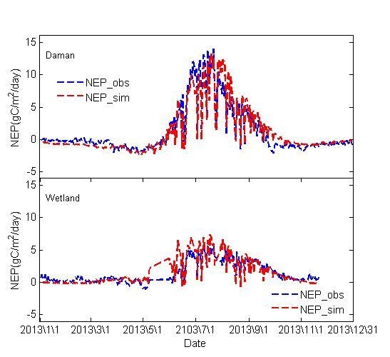
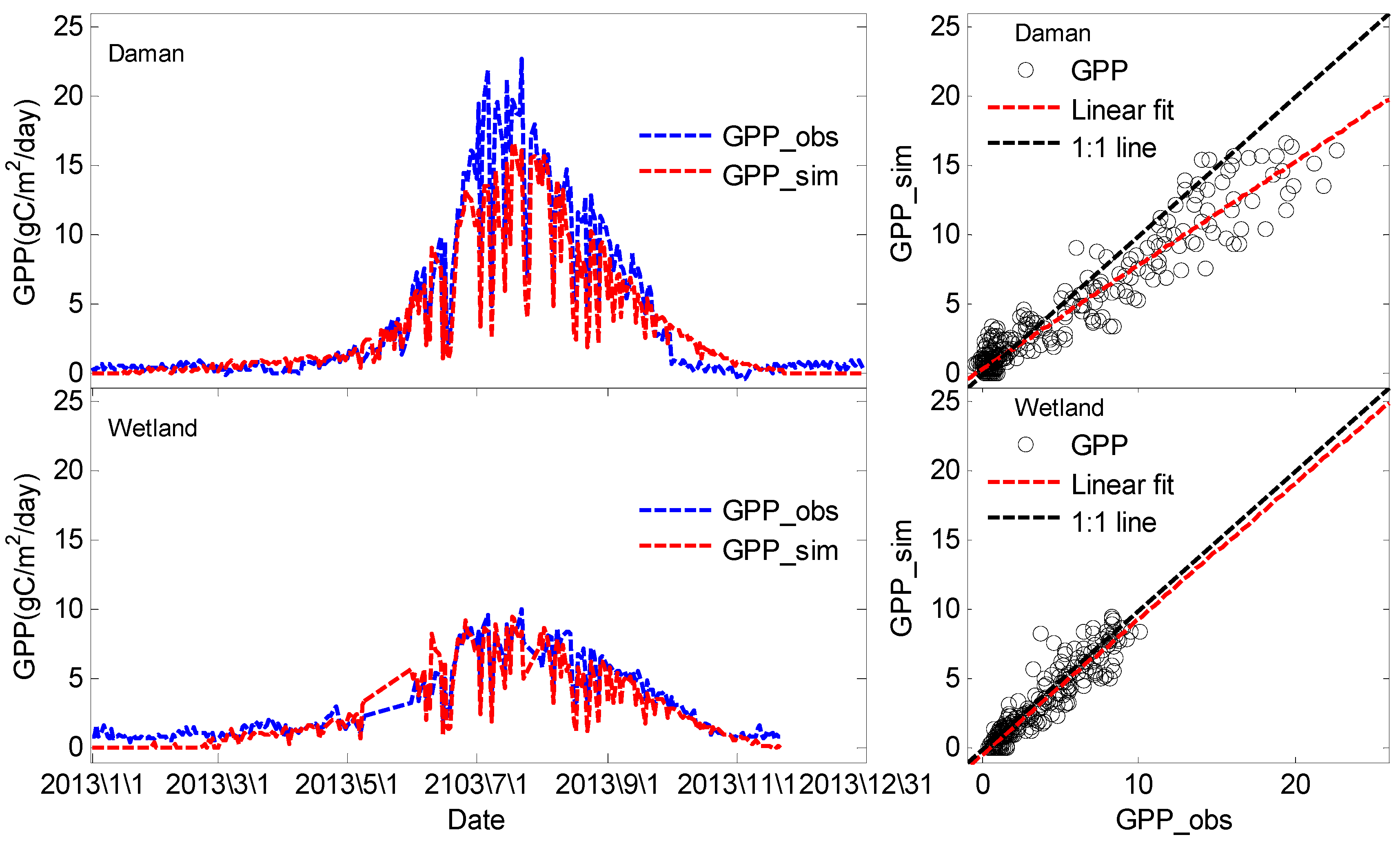
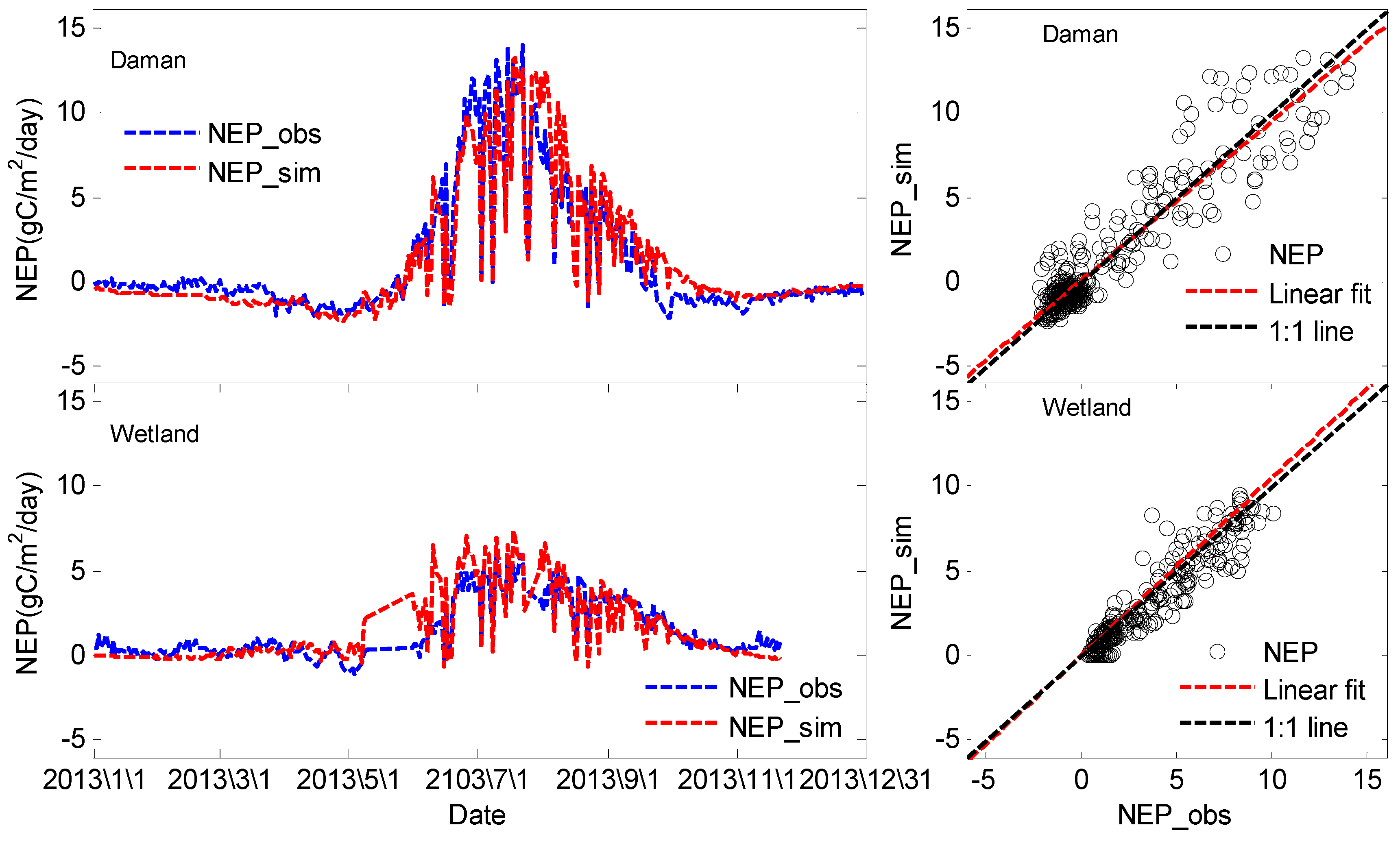
3.3. Carbon Flux Predicted by the RS-CFLUX Model

Figure 6 and Figure 7 show the comparison between the carbon flux predicted by the RS-CFLUX model and the carbon flux estimated from EC at Daman superstation and Zhangye wetland station. The model predictions and observations were consistent. The RS-CFLUX model can correctly simulate the seasonal dynamics and quantities of GPP and NEP at the two stations. R², RMSE and NSE of the GPP between the RS-CFLUX model and EC were, respectively 0.92, 1.96 g C/m²/d and 0.87 at Daman superstation, and 0.94, 1.00 g C/m²/day and 0.85 at Zhangye wetland station. R², RMSE and NSE of the NEP between the RS-CFLUX model and EC were 0.88, 1.31 g C/m²/d and 0.87 at the Daman superstation, and 0.78, 1.02 g C/m²/day and 0.61 at the Zhangye wetland station (see Table 3). The sum of the EC-estimated GPP was 1442.04 g C/m²/year at the Daman superstation and 928.89 g C/m²/year at the Zhangye wetland station (the GPP missed for 68 days in 2013 and was not filled for the Zhangye wetland station); The sum of predicted GPP was 1196.93 g C/m²/year at the Daman superstation and 775.24 g C/m²/year at the Zhangye wetland station at the corresponding time. At the peak-growing season, GPP was obviously underestimated at Daman superstation; this is mainly caused by model parameter LUE_max. LUE_max is smaller when both in-situ GPP and NEE were simultaneously used to calibrate CFLUX model than when only in-situ GPP was used. The sum of the EC-estimated NEP was 409.38 g C/m²/year at the Daman superstation and 422.60 g C/m²/year at the Zhangye wetland station (the GPP missed for 68 days in 2013 were not filled at Zhangye wetland station); The sum of the predicted NEP was 409.46 g C/m²/year at the Daman superstation and 433.12 g C/m²/year at the Zhangye wetland station at the corresponding time. The linear regression slope between the model and observations showed GPP was only slightly underestimated at the Daman superstation.

Figure 6. Validation of the GPP estimated by the RS-CFLUX model at the Daman superstation (Daman) and Zhangye wetland station (Wetland). The slope and residual of the linear fit are shown in Table 3.

Figure 6. Validation of the GPP estimated by the RS-CFLUX model at the Daman superstation (Daman) and Zhangye wetland station (Wetland). The slope and residual of the linear fit are shown in Table 3.

Figure 7. Validation of the NEP estimated by the RS-CFLUX model at the Daman superstation (Daman) and Zhangye wetland station (Wetland). The slope and residual of the linear fit are shown in Table 3.

Figure 7. Validation of the NEP estimated by the RS-CFLUX model at the Daman superstation (Daman) and Zhangye wetland station (Wetland). The slope and residual of the linear fit are shown in Table 3.

Table 3. Comparison of the RS-CFLUX modeled GPP with the observed GPP at the Daman superstation (Daman) and Zhangye wetland station (Wetland).

Stations	Fluxes	R2	RMSE	NSE	Slope	Residue
Daman	GPP	0.92	1.96 (gC/m2/day)	0.87	0.75	0.33 (gC/m2/day)
	NEP	0.88	1.31 (gC/m2/day)	0.87	0.94	0.07 (gC/m2/day)
Wetland	GPP	0.94	1.00 (gC/m2/day)	0.85	0.97	−0.43 (gC/m2/day)
	NEP	0.78	1.02 (gC/m2/day)	0.61	1.05	−0.04 (gC/m2/day)

Table 3. Comparison of the RS-CFLUX modeled GPP with the observed GPP at the Daman superstation (Daman) and Zhangye wetland station (Wetland).

Stations	Fluxes	R2	RMSE	NSE	Slope	Residue
Daman	GPP	0.92	1.96 (gC/m2/day)	0.87	0.75	0.33 (gC/m2/day)
	NEP	0.88	1.31 (gC/m2/day)	0.87	0.94	0.07 (gC/m2/day)
Wetland	GPP	0.94	1.00 (gC/m2/day)	0.85	0.97	−0.43 (gC/m2/day)
	NEP	0.78	1.02 (gC/m2/day)	0.61	1.05	−0.04 (gC/m2/day)

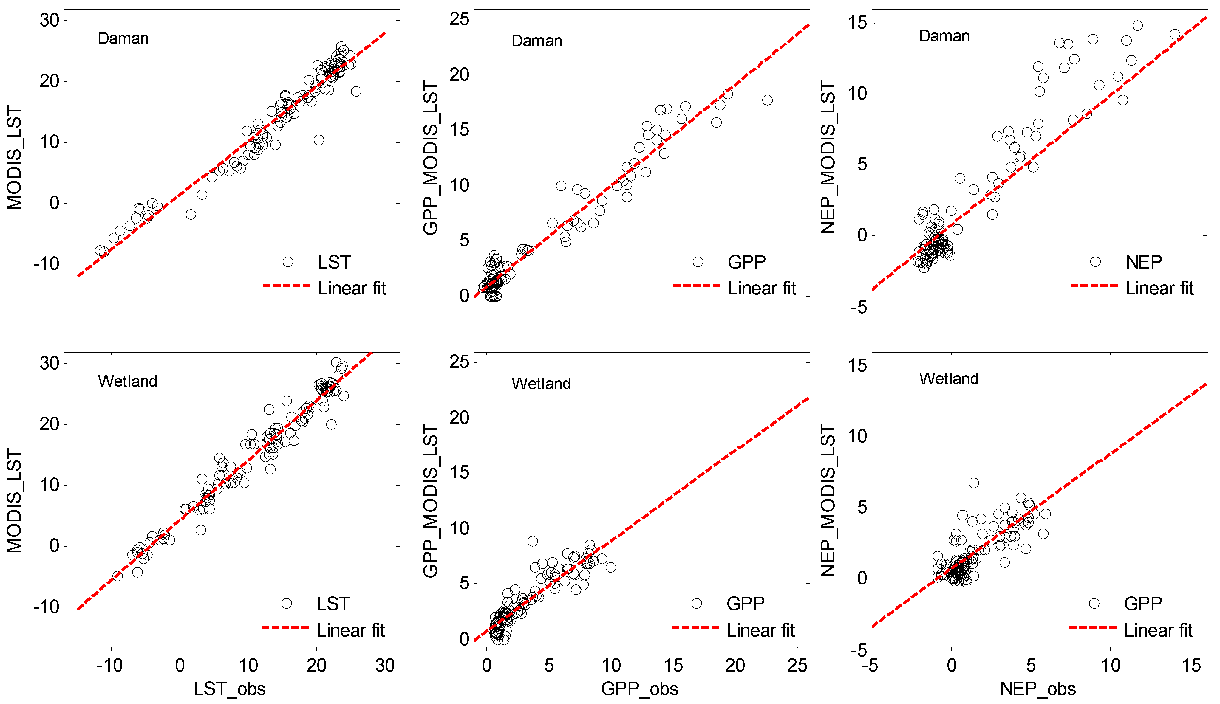
3.4. Using the MODIS LST Product as Input for the RS-CFLUX Model

LST input for the RS-CFLUX model can be replaced with the MODIS LST product. The average of daytime and nighttime LSTs of the MODIS daily LST product MOD11A1 was used as input of RS-CFLUX, and it is compared with the daily average in-situ LST (see left column of Figure 7 and Table 4). MODIS LST has a large positive bias comparing with in-situ LST at the Zhangye wetland station, but little bias at the Daman superstation. This is attributed to the strong land surface heterogeneity at Zhangye wetland station. When the average daytime and nighttime LSTs of MOD11A1 were used as input for RS-CFLUX at the Daman superstation and Zhangye wetland station, the RS-CFLUX model performed well at both stations (see middle and right columns of Figure 8 and Table 4).

Figure 8. Validation of the RS-CFLUX model using MODIS LST as input at the Daman superstation (Daman) and Zhangye wetland station (Wetland). The slope and residual of the linear fit are shown in Table 4.

Figure 8. Validation of the RS-CFLUX model using MODIS LST as input at the Daman superstation (Daman) and Zhangye wetland station (Wetland). The slope and residual of the linear fit are shown in Table 4.

Table 4. Results from the RS-CFLUX model using MODIS LST as input.

Variables	R2	RMSE	NSE	Slope	Residue
Daman_LST	0.98	2.25 (°C)	0.94	0.89	1.4 (°C)
Wetland_LST	0.90	4.56 (°C)	0.75	0.98	4.3 (°C)
Daman_GPP	0.96	1.37 (gC/m2/d)	0.94	0.92	0.77 (gC/m2/d)
Wetland_GPP	0.93	1.11 (gC/m2/d)	0.82	0.81	0.71 (gC/m2/d)
Daman_NEP	0.75	2.03 (gC/m2/d)	0.72	0.92	0.77 (gC/m2/d)
Wetland_NEP	0.72	1.15 (gC/m2/d)	0.56	0.74	0.68 (gC/m2/d)

Table 4. Results from the RS-CFLUX model using MODIS LST as input.

Variables	R2	RMSE	NSE	Slope	Residue
Daman_LST	0.98	2.25 (°C)	0.94	0.89	1.4 (°C)
Wetland_LST	0.90	4.56 (°C)	0.75	0.98	4.3 (°C)
Daman_GPP	0.96	1.37 (gC/m2/d)	0.94	0.92	0.77 (gC/m2/d)
Wetland_GPP	0.93	1.11 (gC/m2/d)	0.82	0.81	0.71 (gC/m2/d)
Daman_NEP	0.75	2.03 (gC/m2/d)	0.72	0.92	0.77 (gC/m2/d)
Wetland_NEP	0.72	1.15 (gC/m2/d)	0.56	0.74	0.68 (gC/m2/d)

4. Discussions

4.1. Comparison of the Carbon Flux

Farmlands and wetlands are the two most productive ecosystems in the midstream of the Heihe River Basin. During the peak of the growing season, the GPP and NEP obviously higher at the Daman superstation than the Zhangye wetland station. However, the GPP and NEP were slightly lower at the Daman superstation than the Zhangye wetland station at the beginning and end of the growing season. Maize at the Daman superstation is usually sown in late April and harvested in late September, and it has faster growth speed than reed. However, reed at the Zhangye wetland station usually begins to sprout in early April and wither in early October. The yearly GPP was obviously higher at the Daman superstation than at the Zhangye wetland station. Because maize is C4 plant which has higher light use efficiency than C3, and maize land is fertilized and irrigated by farmers. The NEP value of the Daman superstation and Zhangye wetland station were nearly equal. Thus, the ecosystem respiration of the Daman superstation was also higher than that of the Zhangye wetland station. Under waterlogged conditions, soil respiration is constrained because of the lack of oxygen and reduced porosity due to the high soil water content [36,37]. Another reason is higher GPP at Daman superstation will result in higher autotrophic respiration.

4.2. Uncertainties Resulted from Model Parameters

The model parameters can lead to uncertainties in the results of the RS-CFLUX model. The model calibration suggested that only a few parameters were well constrained. The number of parameters that can be well constrained depends on the amount and quality of measurement that used in calibration. It is also reported by previous study that there are only few parameters can be well constrained when only the carbon flux data was used in the reversion process [38,39]. Based on the probability density function proposed by MCMC for each parameter, we used the Monte Carlo method to assess the uncertainties in the model outputs resulting from each parameter (see Figure 9 and Figure 10). LUE_max resulted in the greatest uncertainties in GPP, followed by LST_opt. LST_min and LST_max both resulted in low uncertainties in the GPP. Rref, E0 and a did not result in uncertainties in the GPP prediction. However, E0, Rref and LUE_max led to the greatest uncertainties in the NEP, followed by LST_opt and a. LST_min and LST_max led to low uncertainties in the NEP prediction. In addition to the parameters, forcing variables and model structure also resulted in uncertainties in the model outputs [40]. Observation instruments contain stochastic error. Furthermore, data processing also results in errors. The model is a simple function with a few environmental factors; it does not include all exchange processes between the ecosystem and atmosphere [41].

Figure 9. Uncertainties in the GPP caused by parameters in the RS-CFLUX model. N (mu, delta) is a normal distribution with a mean mu and standard deviation delta.

Figure 9. Uncertainties in the GPP caused by parameters in the RS-CFLUX model. N (mu, delta) is a normal distribution with a mean mu and standard deviation delta.

Figure 10. Uncertainties in the NEP caused by parameters in the RS-CFLUX model. N (mu, delta) is a normal distribution with a mean mu and standard deviation delta.

Figure 10. Uncertainties in the NEP caused by parameters in the RS-CFLUX model. N (mu, delta) is a normal distribution with a mean mu and standard deviation delta.

4.3. Potential to be a Fully Remote Sensing Base Carbon Flux Model

Generally, the RS-CFLUX model performed well in both the Daman superstation and Zhangye wetland station. The model correctly estimated the GPP and NEP of the ecosystem. The model accuracy in term of RMSE and R² is as high as the other model used in this area, such as VPM [19]. Based on in-situ data, it is found that correlation coefficient between LST and NEE is much higher than that between air temperature and NEE. Furthermore, high-resolution LST and PAR data could be retrieved from remote sensing data; this will improve the carbon fluxes estimation at the areas with sparse weather stations, such as Northwest China. When using the remote-sensing-derived PAR product and LST product as inputs, RS-CFLUX will simulate the carbon flux using only remote sensing data. However, high temporal resolution PAR and LST products are difficult to generate. A lot of LST value is missing in current MODIS LST product because of the impact of the weather. Some methods are developed in recent years, which can be used to reconstruct the LST product and form a time continuous LST [42]. Polar orbiting and geostationary satellite data can be combined with other remote sensing data to generate continuous daily even hourly PAR data. If the quality of remote sensing data product is improved using these new data and method, then the RS-CFLUX model could easily estimate the carbon flux at regional scale.

5. Conclusions

In summary, carbon fluxes model based on remote sensing data were presented in this study. The model was calibrated and validated at two stations in the midstream of the Heihe River Basin. Based on this research, the following conclusions are presented. (1) In the midstream of the Heihe River Basin, the maize land had higher GPP (1442.04 g C/m²/year) than the reed dominated wetland (928.89 g C/m²/year). However, the NEP of maize land (409.38 g C/m²/year) was nearly equal to that of the reed dominated wetland (422.60 g C/m²/year). (2) RS-CFLUX can adequately simulate the seasonal dynamics and quantity of carbon fluxes for the maize land and reed dominated wetland. (3) From the calibration of RS-CFLUX, only a few parameters were well constrained. However, these well-constrained parameters are important to model output, such as the maximum light use efficiency, respiration at the reference temperature and the activation energy parameter of respiration. If these parameters are not well estimated, then they can result in large uncertainties in the model output.

References

1. Falkowski, P.; Scholes, R.J.; Boyle, E.; Canadell, J.; Canfield, D.; Elser, J.; Gruber, N.; Hibbard, K.; Högberg, P.; Linder, S.; et al. The global carbon cycle: A test of our knowledge of earth as a system. Science 2000, 290, 291–296. [Google Scholar] [CrossRef] [PubMed]
2. Bonan, G.B. Forests and climate change: Forcings, feedbacks, and the climate benefits of forests. Science 2008, 320, 1444–1449. [Google Scholar] [CrossRef] [PubMed]
3. Beer, C.; Reichstein, M.; Tomelleri, E.; Ciais, P.; Jung, M.; Carvalhais, N.; Rödenbeck, C.; Arain, M.A.; Baldocchi, D.; Bonan, G.B.; et al. Terrestrial gross carbon dioxide uptake: Global distribution and covariation with climate. Science 2010, 329, 834–838. [Google Scholar] [CrossRef] [PubMed]
4. Ueyama, M.; Harazono, Y.; Kim, Y.; Tanaka, N. Response of the carbon cycle in sub-arctic black spruce forests to climate change: Reduction of a carbon sink related to the sensitivity of heterotrophic respiration. Agr. Forest Meteorol. 2009, 149, 582–602. [Google Scholar] [CrossRef]
5. Longbottom, T.L.; Townsend-Small, A.; Owen, L.A.; Murari, M.K. Climatic and topographic controls on soil organic matter storage and dynamics in the Indian Himalaya: Potential carbon cycle-climate change feedbacks. Catena 2014, 119, 125–135. [Google Scholar] [CrossRef]
6. Prince, S.D.; Goward, S.N. Global primary production: A remote sensing approach. J. Biogeogr. 1995, 22, 815–835. [Google Scholar] [CrossRef]
7. Veroustraete, F.; Sabbe, H.; Eerens, H. Estimation of carbon mass fluxes over Europe using the C-Fix model and EuroFlux data. Remote Sens. Environ. 2002, 83, 376–399. [Google Scholar] [CrossRef]
8. Lu, L.; Li, X.; Veroustraete, F.; Kang, E.; Wang, J. Analysing the forcing mechanisms for net primary productivity changes in the Heihe river basin, north-west China. Int. J. Remote Sens. 2009, 30, 793–816. [Google Scholar] [CrossRef]
9. Xiao, X.; Zhang, Q.; Braswell, B.; Urbanski, S.; Boles, S.; Wofsy, S.; Moore Iii, B.; Ojima, D. Modeling gross primary production of temperate deciduous broadleaf forest using satellite images and climate data. Remote Sens. Environ. 2004, 91, 256–270. [Google Scholar] [CrossRef]
10. Running, S.W.; Nemani, R.R.; Heinsch, F.A.; Zhao, M.; Reeves, M.; Hashimoto, H. A continuous satellite-derived measure of global terrestrial primary production. Bioscience 2004, 54, 547–560. [Google Scholar] [CrossRef]
11. Xiao, J.; Davis, K.J.; Urban, N.M.; Keller, K.; Saliendra, N.Z. Upscaling carbon fluxes from towers to the regional scale: Influence of parameter variability and land cover representation on regional flux estimates. J. Geophys. Res.: Biogeosci. 2011, 116. [Google Scholar] [CrossRef]
12. Sánchez, J.M.; Kustas, W.P.; Caselles, V.; Anderson, M.C. Modelling surface energy fluxes over maize using a two-source patch model and radiometric soil and canopy temperature observations. Remote Sens. Environ. 2008, 112, 1130–1143. [Google Scholar] [CrossRef]
13. Blum, M.; Lensky, I.M.; Nestel, D. Estimation of olive grove canopy temperature from MODIS thermal imagery is more accurate than interpolation from meteorological stations. Agr. Forest Meteorol. 2013, 176, 90–93. [Google Scholar] [CrossRef]
14. Cheng, G.D.; Li, X.; Zhao, W.Z.; Xu, Z.M.; Feng, Q.; Xiao, S.C.; Xiao, H.L. Integrated study of the water-ecosystem-economy in the Heihe River Basin. Natl. Sci. Rev. 2014, 1, 413–428. [Google Scholar] [CrossRef]
15. Li, X.; Cheng, G.; Liu, S.; Xiao, Q.; Ma, M.; Jin, R.; Che, T.; Liu, Q.; Wang, W.; Qi, Y.; et al. Heihe watershed allied telemetry experimental research (HiWATER): Scientific objectives and experimental design. Bull. Amer. Meteor. Soc. 2013, 94, 1145–1160. [Google Scholar] [CrossRef]
16. Xu, Z.; Liu, S.; Li, X.; Shi, S.; Wang, J.; Zhu, Z.; Xu, T.; Wang, W.; Ma, M. Intercomparison of surface energy flux measurement systems used during the HiWATER-MUSOEXE. J. Geophys. Res.: Atmos. 2013, 118, 13140–13157. [Google Scholar] [CrossRef]
17. Liu, S.M.; Xu, Z.W.; Wang, W.Z.; Jia, Z.Z.; Zhu, M.J.; Bai, J.; Wang, J.M. A comparison of eddy-covariance and large aperture scintillometer measurements with respect to the energy balance closure problem. Hydrol. Earth Syst. Sci. 2011, 15, 1291–1306. [Google Scholar] [CrossRef]
18. Liu, S.M.; Xu, Z.W.; Zhu, Z.L.; Jia, Z.Z.; Zhu, M.J. Measurements of evapotranspiration from eddy-covariance systems and large aperture scintillometers in the Hai River Basin, China. J. Hydrol. 2013, 487, 24–38. [Google Scholar] [CrossRef]
19. Wang, X.; Ma, M.; Huang, G.; Veroustraete, F.; Zhang, Z.; Song, Y.; Tan, J. Vegetation primary production estimation at maize and alpine meadow over the Heihe River Basin, China. Int. J. Appl. Earth Obs. Geoinf. 2012, 17, 94–101. [Google Scholar] [CrossRef]
20. Wang, X.; Ma, M.; Li, X.; Song, Y.; Tan, J.; Huang, G.; Zhang, Z.; Zhao, T.; Feng, J.; Ma, Z.; et al. Validation of MODIS-GPP product at 10 flux sites in Northern China. Int. J. Remote Sens. 2012, 34, 587–599. [Google Scholar] [CrossRef]
21. Vermote, E.F.; Vermeulen, A. Atmospheric correction algorithm: Spectral reflectances (MOD09). Available online: http://modis.gsfc.nasa.gov/data/atbd/atbd_mod08.pdf (accessed on 17 December 2014).
22. Wan, Z.M. MODIS Land-Surface Temperature Algorithm Theoretical Basis Document (LST ATBD). 1999. Available online: http://modis.gsfc.nasa.gov/data/atbd/atbd_mod11.pdf (accessed on 17 December 2014). [Google Scholar]
23. Chen, J.; Jonsson, P.; Tamura, M.; Gu, Z.; Matsushita, B.; Eklundh, L. A simple method for reconstructing a high-quality NDVI time-series data set based on the Savitzky-Golay filter. Remote Sens. Environ. 2004, 91, 332–344. [Google Scholar] [CrossRef]
24. Geng, L.; Ma, M.; Wang, X.; Yu, W.; Jia, S.; Wang, H. Comparison of eight techniques for reconstructing multi-satellite sensor time-series NDVI data sets in the Heihe River Basin, China. Remote Sens. 2014, 6, 2024–2049. [Google Scholar] [CrossRef]
25. Ma, M.; Veroustraete, F. Reconstructing pathfinder AVHRR land NDVI time-series data for the northwest of China. Adv. Space Res. 2006, 37, 835–840. [Google Scholar] [CrossRef]
26. Huete, A.; Didan, K.; Miura, T.; Rodriguez, E.P.; Gao, X.; Ferreira, L.G. Overview of the radiometric and biophysical performance of the MODIS vegetation indices. Remote Sens. Environ. 2002, 83, 195–213. [Google Scholar] [CrossRef]
27. Rahman, A.F.; Sims, D.A.; Cordova, V.D.; El-Masri, B.Z. Potential of MODIS EVI and surface temperature for directly estimating per-pixel ecosystem C Fluxes. Geophys. Res. Lett. 2005, 32. [Google Scholar] [CrossRef]
28. Tian, H.; Melillo, J.M.; Kicklighter, D.W.; McGuire, A.D.; Helfrich, J. The sensitivity of terrestrial carbon storage to historical climate variability and atmospheric CO2 in the United States. Tellus B 1999, 51, 414–452. [Google Scholar] [CrossRef]
29. Gao, B.-C. NDWI—A normalized difference water index for remote sensing of vegetation liquid water from space. Remote Sens. Environ. 1996, 58, 257–266. [Google Scholar] [CrossRef]
30. Lloyd, J.; Taylor, J.A. On the temperature dependence of soil respiration. Funct. Ecol. 1994, 8, 315–323. [Google Scholar] [CrossRef]
31. Xu, T.; White, L.; Hui, D.; Luo, Y. Probabilistic inversion of a terrestrial ecosystem model: Analysis of uncertainty in parameter estimation and model prediction. Glob. Biogeochem. Cycles 2006, 20. [Google Scholar] [CrossRef]
32. Wu, X.; Luo, Y.; Weng, E.; White, L.; Ma, Y.; Zhou, X. Conditional inversion to estimate parameters from eddy-flux observations. J. Plant. Ecol. 2009, 2, 55–68. [Google Scholar] [CrossRef]
33. Gelman, A.; Rubin, D.B. Inference from iterative simulation using multiple sequences. Statist. Sci. 1992, 7, 457–472. [Google Scholar] [CrossRef]
34. Drolet, G.; Middleton, E.; Huemmrich, K.; Hall, F.; Amiro, B.; Barr, A.; Black, T.; McCaughey, J.; Margolis, H. Regional mapping of gross light-use efficiency using MODIS spectral indices. Remote Sens. Environ. 2008, 112, 3064–3078. [Google Scholar] [CrossRef]
35. Singsaas, E.L.; Ort, D.R.; DeLucia, E.H. Variation in measured values of photosynthetic quantum yield in ecophysiological studies. Oecologia 2001, 128, 15–23. [Google Scholar] [CrossRef]
36. Holden, J. Peatland hydrology and carbon release: Why small-scale process matters. Philos. Trans. R. Soc. A Math. Phys. Eng. Sci. 2005, 363, 2891–2913. [Google Scholar] [CrossRef]
37. Kayranli, B.; Scholz, M.; Mustafa, A.; Hedmark, Å. Carbon storage and fluxes within freshwater wetlands: A critical review. Wetlands 2010, 30, 111–124. [Google Scholar] [CrossRef]
38. Wang, Y.-P.; Leuning, R.; Cleugh, H.A.; Coppin, P.A. Parameter estimation in surface exchange models using nonlinear inversion: How many parameters can we estimate and which measurements are most useful? Glob. Chang. Biol. 2001, 7, 495–510. [Google Scholar] [CrossRef]
39. Yuan, W.; Liang, S.; Liu, S.; Weng, E.; Luo, Y.; Hollinger, D.; Zhang, H. Improving model parameter estimation using coupling relationships between vegetation production and ecosystem respiration. Ecol. Model. 2012, 240, 29–40. [Google Scholar] [CrossRef]
40. Ren, X.; He, H.; Moore, D.J.P.; Zhang, L.; Liu, M.; Li, F.; Yu, G.; Wang, H. Uncertainty analysis of modeled carbon and water fluxes in a subtropical coniferous plantation. J. Geophys. Res.: Biogeosci. 2013, 118, 1674–1688. [Google Scholar] [CrossRef]
41. McCallum, I.; Wagner, W.; Schmullius, C.; Shvidenko, A.; Obersteiner, M.; Fritz, S.; Nilsson, S. Satellite-based terrestrial production efficiency modeling. Carbon Balanc. Manag. 2009, 4. [Google Scholar] [CrossRef]
42. Xu, Y.; Shen, Y. Reconstruction of the land surface temperature time series using harmonic analysis. Comput. Geosci. 2013, 61, 126–132. [Google Scholar] [CrossRef]