Spatiotemporal Variation in Surface Urban Heat Island Intensity and Associated Determinants across Major Chinese Cities

Abstract

Urban heat islands (UHIs) created through urbanization can have negative impacts on the lives of people living in cities. They may also vary spatially and temporally over a city. There is, thus, a need for greater understanding of these patterns and their causes. While previous UHI studies focused on only a few cities and/or several explanatory variables, this research provides a comprehensive and comparative characterization of the diurnal and seasonal variation in surface UHI intensities (SUHIIs) across 67 major Chinese cities. The factors associated with the SUHII were assessed by considering a variety of related social, economic and natural factors using a regression tree model. Obvious seasonal variation was observed for the daytime SUHII, and the diurnal variation in SUHII varied seasonally across China. Interestingly, the SUHII varied significantly in character between northern and southern China. Southern China experienced more intense daytime SUHIIs, while the opposite was true for nighttime SUHIIs. Vegetation had the greatest effect in the day time in northern China. In southern China, annual electricity consumption and the number of public buses were found to be important. These results have important theoretical significance and may be of use to mitigate UHI effects.

1. Introduction

Rapid urbanization has made urban climate change more dramatic than global climate change [1]. One consequence for urban environments is the urban heat island (UHI) effect, whereby urban centers experience higher temperatures than the surrounding rural areas [2]. As a local phenomenon [3,4,5], UHIs can affect directly the lives of urban residents, as indicated by the high demand for air-conditioning [6], high rates of heat-related disease [7], and the amount of pollution in urban areas [8,9,10]. Thus, mitigating UHI effects should be considered in urban planning, and greater understanding of the patterns and specific causes of the UHI effect is required in order to take appropriate mitigation measures.

In situ data were often used in early UHI studies. However, in situ data are usually private or subject to governmental restrictions and are costly to obtain, especially for large-area analyses [11]. Furthermore, the sparse and limited spatial coverage of in situ data make them unsuitable for identifying the spatial patterns of UHIs across different cities [11,12]. Remote sensing (RS) technology provides a practical and promising technique for monitoring UHIs [13,14,15]. The land surface temperature (LST) derived from thermal infrared (TIR) remote sensing images was used to describe the surface UHI (SUHI). LST data have an important role in SUHI studies due to the potentially large-area and repeat nature of the coverage. Numerous RS-based SUHI studies have documented the spatial patterns of intra-city SUHIs and their relationship with urban surface properties [16], such as urban population [17], urban land use/land cover [18,19,20,21], vegetation coverage [22], and anthropogenic heat release [23]. A few SUHI studies based on MODerateresolution Imaging Spectroradiometer (MODIS) LST at the regional or global scale were also reported in recent years. For example, [24] undertook a comparative analysis of the spatial patterns and seasonal cycles of SUHIs and their relationships with building density, population and vegetation cover for the period 2001 to 2003 in five temperate and three tropical mega-cities. [25] assessed the relationship between the skin temperature amplitude and ecological settings for the 38 most populous cities in the United States. [26] determined the seasonal variation of the SUHI in nine European cities, while [27] explored diurnal variation in the intensity of the SUHI (SUHII) across 419 large global cities.

Such SUHI studies at regional or global scale can provide a comparative understanding of SUHIs. However, most of this research focused on specific aspects of the urban system (often the vegetation) when exploring the possible factors contributing to the SUHI. As each city is a complex, natural, economic and ecological system [28], considering only a few factors may miss important properties and ignore the integrated effect of multiple factors (i.e., their interactions) [29]. [30] treated urban areas as ecological systems and then determined quantitatively the social and ecological factors affecting UHIs using measurements from meteorological stations in major Chinese cities. However, the relative importance of each factor was not reported. Besides, other variables measuring urban form, such as compactness and porosity, may also be related to SUHIs, as urban form can affect lifestyle and transport behaviors [31]. However, few studies have quantified their contributions to SUHI, with the exception of form in the canopy layer, which is well studied.

China has experienced rapid urbanization in the last decade. At the end of 2010 nearly half of the Chinese population lived in urban areas, an increase of 13.5% since 2000 (National Bureau of Statistics of China, 2011). Urban expansion and shrinking cropland were also characterized [32]. Increasing urban populations and urban areas have brought a series of urban environmental consequences, among which UHIs are one of the most well-known [33,34]. Thus, taking China as the study area, this research aimed to fill the above-mentioned research gaps and provide a comprehensive and comparative understanding of the spatiotemporal patterns of SUHIs and their associated factors in a large set of major Chinese cities. Specifically, the objectives of this research were: (i) to compare the spatiotemporal patterns of SUHI intensity (SUHII) in major Chinese cities; and (ii) to identify the factors associated with SUHII by considering a series of social, economic and natural factors, taking the urban extent as a complex ecological system.

2. Data and Methods

2.1. Study Area

Following Peng et al. [27], this research selected all Chinese cities with a population larger than one million in 2007 as defining the study area. After cities with incomplete statistical data for the 2003 to 2010 period were excluded, 67 major cities in China were selected (Figure 1). The location of each city was determined using a geographical database [35]. The Qinling Mountains-Huaihe River Line is the geographical dividing line between northern China and southern China [36].

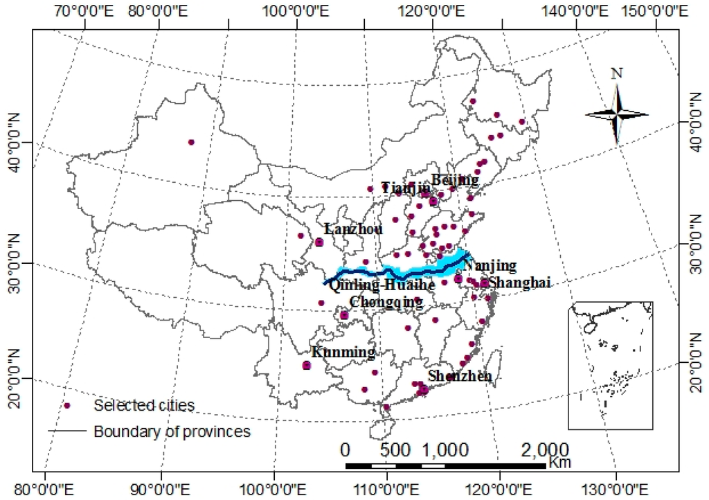
Figure 1. Sixty-seven selected cities in this research. The eight labeled cities are typical cities discussed in the text.

Figure 1. Sixty-seven selected cities in this research. The eight labeled cities are typical cities discussed in the text.

2.2. Data

2.2.1. Satellite Sensor Data

MODIS data (Collection 5), including MYD11A2 (8-day, 1000 m, land surface temperature/emissivity), MYD13A3 (monthly, 1000 m, vegetation indices), and MCD43B3 (16-day, 1000 m, albedo), were obtained from the National Aeronautics and Space Administration (NASA) Reverb portal [37]. The MYD11A2 data were used to derive the time-series of LST. This dataset included both the instantaneous daytime (local time at 1:30 pm) and nighttime (local time at 1:30 am) temperature information. It has high accuracy and low root mean square error(RMSE) according to surface emissivity evaluations [27]. In this research, invalid pixels were further eliminated using the quality assurance (QA) flags included in the dataset. NDVI and albedo data were also derived from MYD13A3 and MCD43B3, respectively, excluding bad pixels using the available QA information.

Version 4 of the annual global stable nighttime lights dataset from the Defense Meteorological Satellite Program/Operational Lines can System (DMSP/OLS) during the period 2003 and 2010 was acquired from the National Geophysical Data Center/Earth Observation Group (NGDC/EOG) [38]. These images were derived from grid-based annual visible bands with digital numbers ranging from 0 to 63 and a spatial resolution of approximately 1 km. They were used to extract the urban built-up boundaries of the selected cities in China.

2.2.2. Demographic Data

City-level statistical data were derived from the China cities’ Statistical Yearbooks. Detailed information on the selected variables is given in Section 2.3.2. The demographic and socioeconomic data were acquired at the urban level and can be matched with the SUHIIs measured with the built-up area derived from DMSP/OLS images [39].

2.3. Methodology

2.3.1. SUHII Calculation

The SUHI intensity (SUHII) is calculated as the difference in LST between an urban region and the surrounding rural region according to the calculation of UHII by Oke et al. [40]. In this research, the original 8-day daytime (local time at 1:30 pm) and nighttime (local time at 1:30 am) MODIS LSTs were firstly averaged monthly. To produce the monthly LST, the original Julian day used in the MODIS product was converted to calendar format, and then the MODIS LST images in the same month were averaged. Subsequently, the monthly LST was seasonally averaged during the period 2003 and 2010. The four seasons were defined as spring (March to May), summer (June to August), autumn (September to November), and winter (December to February). Secondly, the urban areas were extracted from the DMSP/OLS nighttime lights images using the threshold method [41]. The rural areas were then defined as the equal-area buffering zone of the urban area following Peng et al. [27], and the seasonally averaged LST in urban areas and rural areas for each city was calculated. The seasonally averaged SUHIIs for each city during the period 2003 and 2010 were obtained by subtracting the averaged LST over the rural area from that over urban areas.

2.3.2. Explanatory Variables Selection

According to [3], a series of factors contribute to SUHIs, including geographical location, time, synoptic weather, city size, city function, and city form. Those controllable variables have attracted the most attention in SUHI studies, as they can be used to take measures to mitigate SUHI effects. In this research, we selected relevant controllable factors to analyze their relative contribution in the urban system. For convenience, all the factors selected were grouped into three categories: (i) anthropogenic heat discharge factors, (ii) land surface descriptors and (iii) urban form indicators.

We considered six indicators to reflect the human-induced heat discharge, including gross domestic product (GDP), annual electricity consumption, water consumption, liquefied petroleum gas (LPG) supply, number of public buses, and number of taxis at the end of the year.

Both continuous index variables from remotely sensed images and discrete variables from statistical yearbooks were used to describe the land surface characteristics. For the spatially continuous variables, NDVI and albedo were firstly seasonally averaged and the differences between the urban and rural areas were calculated, named as ΔNDVI and Δalbedo. The discrete parameters included the road area at the end of the year and the size of the built-up area.

Urban forms can be defined according to the spatial pattern of human activities and can be measured in different dimensions [42,43]. In this research, three distinct dimensions were used to describe the urban spatial form: porosity, density and compactness [44]. Porosity is the ratio of open space to the total urban area where open space is the sum of green and construction areas. Both variables, together with the population density, were derived directly from statistical yearbooks. Compactness was calculated based on the urban patches extracted from the DMSP/OLS nighttime lights images using the following formula [45]:

$$CI=2\times \sqrt{\pi \times A}/P$$

(1)

where, CI is compactness; A and P are the area and perimeter of the urban patches, respectively. The value ranges from 1 for roundness (the most compact shape) to 0 for line (the least compact shape). The larger the compactness value, the more compact the city.

Table 1. Selected variables related to SUHII.

Code	Name of Indicator	Unit	Source
A1	Annual electricity consumption	kWh	Statistical yearbook
A2	LPG gas supply	Ton	Statistical yearbook
A3	Annual water consumption	10,000 m3	Statistical yearbook
A4	Number of public buses	Vehicle	Statistical yearbook
A5	Number of taxis	Vehicle	Statistical yearbook
A6	GDP of the built-up area	RMB yuan	Statistical yearbook
L1	Road area at the end of the year	10,000 m2	Statistical yearbook
L2	Size of built-up area	Ha	Statistical yearbook
L3	ΔΔNDVI	-	MODIS product
L4	ΔAlbedo	-	MODIS product
U1	Green area of built-up area	%	Statistical yearbook
U2	Population density	Person per ha	Statistical yearbook
U3	Construction area coverage	%	Statistical yearbook
U4	Compactness	-	DMSP/OLS

A: anthropogenic heat discharge; L: land surface descriptors; U: urban form indicator.

Table 1. Selected variables related to SUHII.

Code	Name of Indicator	Unit	Source
A1	Annual electricity consumption	kWh	Statistical yearbook
A2	LPG gas supply	Ton	Statistical yearbook
A3	Annual water consumption	10,000 m3	Statistical yearbook
A4	Number of public buses	Vehicle	Statistical yearbook
A5	Number of taxis	Vehicle	Statistical yearbook
A6	GDP of the built-up area	RMB yuan	Statistical yearbook
L1	Road area at the end of the year	10,000 m2	Statistical yearbook
L2	Size of built-up area	Ha	Statistical yearbook
L3	ΔΔNDVI	-	MODIS product
L4	ΔAlbedo	-	MODIS product
U1	Green area of built-up area	%	Statistical yearbook
U2	Population density	Person per ha	Statistical yearbook
U3	Construction area coverage	%	Statistical yearbook
U4	Compactness	-	DMSP/OLS

A: anthropogenic heat discharge; L: land surface descriptors; U: urban form indicator.

The full set of variables is summarized in Table 1. Note that the variables have different definitions and units. To eliminate differences between the variables, each variable was normalized by dividing the original series by its mean value, using the formula [30]:

$$\{x^{(1)}(1),x^{(1)}(2)\mathrm{...}{x}^{(1)}(n)\}=\{\frac{x^{(0)}(1)}{{\overline{x}}^0},\frac{x^{(0)}(2)}{{\overline{x}}^0}\mathrm{...}\frac{x^{(0)}(n)}{{\overline{x}}^0}\}$$

(2)

where, x⁽⁰⁾(n) is the original data; n denotes the number of data for each factor; x⁽¹⁾(n) is the value of equalization treatment to x⁽¹⁾(n); and ${\overline{x}}^0$ is the mean value of the original data series.

2.3.3. Regression Tree Model

The regression tree model is a machine-learning method that can produce rule-based models containing more than one rule. Each rule is a multivariate linear regression sub-model that is subject to a set of conditions [46,47,48]. It is useful for estimating a case target value in terms of its attribute values. In this research, the rule-based SUHII model was generated based on a modified regression tree algorithm implemented in the Cubist commercial software linked to R, an open-source statistical computing software environment. The model requires that each case has a target variable (here it was SUHII) and other attributes that provide information that may help to predict the target value. Cubist builds a piecewise linear regression model containing one or more rules to form a conjunction of conditions with a linear expression. Selection of variables to form a piecewise regression is a recursive “training” process. It is trained by dividing the source set into subsets based on the dependent variables. This process is repeated and will be terminated if no more variables are added to the prediction model. In this context, a rule means that if a case satisfies all of the conditions then the linear expression is appropriate for predicting the target value. This model can be expressed in the following equation:

$$y=\{\begin{array}{ccc}{\alpha }_1+{\beta }_{11}{x}_1+\cdots +{\beta }_{1i}{x}_i+{\epsilon }_1& if& x_i\le T_{1i}\\ {\alpha }_2+{\beta }_{21}{x}_1+\cdots +{\beta }_{2i}{x}_i+{\epsilon }_2& if& T_{1i}<x_i\le T_{2i}\\ & \mathrm{...}& \\ {\alpha }_k+{\beta }_{k1}{x}_1+\cdots +{\beta }_{ki}{x}_i+{\epsilon }_k& if& T_{ki}<x_i\end{array}$$

(3)

where y is the target variable; x_i denotes a series of explanatory variables.kis the number of rules, which varies with the model output; T is the conditional value. The model is a multiple linear regression in this research and there can be more than one variable in each rule.

The Cubist software provides three statistical measures to assess the accuracy of the constructed predictive model: the Pearson’s product-moment correlation coefficient (CC), average error (AE), and relative error (RE). The CC measures association and is, thus, used to measure the precision of prediction. The average error is used to measure the overall bias of the regression tree predictions. It is expressed as:

$${\epsilon }_a=\frac{1}{N}{\displaystyle \sum _{t=1}^N\left|y_t-y_t^{\text{'}}\right|}$$

(4)

where ε_a is the average error; N is the number of observations used to construct the predictive model; and y_t and y^’_t are the actual and predicted values of the relative variables, respectively. The suffix t indicates an index for the observations used to construct the predictive model, which ranges from 1 to N.

The relative error is used to assess the accuracy of prediction amongst several regression trees and is expressed as:

$${\epsilon }_r=\frac{1}{N}{\displaystyle \sum _{t=1}^N\left|y_t-y_t^{\text{'}}\right|}/\frac{1}{N}{\displaystyle \sum _{t=1}^N\left|y_t-\overline{y}\right|}$$

(5)

where ε_r is the relative error; and $\overline{y}$ represents the mean value of the actual relative variable. Here, it was averaged over the observed SUHIIs.

In addition to the above three statistical measures calculated by the Cubist software, the root-mean-square error (RMSE) was calculated to measure the overall accuracy between the predicted and observed SUHIIs.

2.3.4. Statistical Analysis

To provide a comprehensive and comparative understanding of the spatiotemporal patterns of the SUHIIs, both the seasonally averaged daytime (1:30 pm) and nighttime (1:30 am) SUHIIs for selected cities were first presented. Then they were averaged over both northern and southern China and analyzed comparatively using statistical description and significance testing. To identify the most important variables for determining SUHIs, rule-based SUHII models were established using the Cubist software. Considering the direct effect of high temperatures on human comfort in summer and the different characteristics of the daytime and nighttime SUHIIs between northern and southern China, four models were applied, including Models 1 (for daytime summer SUHIIs in northern China), 2 (for daytime summer SUHIIs in southern China), 3 (for nighttime summer SUHIIs in northern China) and 4 (for nighttime summer SUHIIs in southern China). All the datasets were divided into two parts; the training set (2003–2008) to build the model and the test set (2009–2010) to evaluate the model. A discussion on both the qualitative and quantitative results is provided below. Figure 2 summarizes the data used and the methodology.

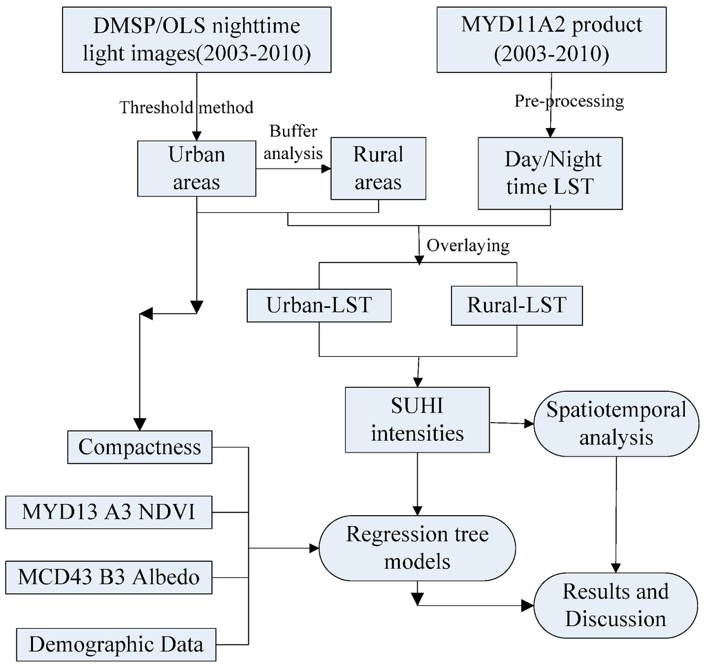
Figure 2. Flowchart describing the research methodology.

Figure 2. Flowchart describing the research methodology.

3. Results

3.1. Diurnal and Seasonal Variation in SUHIIs

Both the seasonally and annually averaged daytime and nighttime SUHIIs during the period 2003 to 2010 for each city are shown in Figure 3. Distinct differences can be found between northern and southern China, especially for the nighttime SUHIIs. Generally, the nighttime SUHIIs in northern China were greater than those in southern China. For the daytime SUHIIs, the patterns were more complex, but it can be seen that the seasonally averaged SUHIIs were greater in southern China, especially in winter. The seasonally averaged daytime and nighttime SUHIIs and the variances over northern and southern China are listed in Table 2. The daytime SUHIIs exhibited distinct seasonal variation, with the largest SUHIIs in summer and smallest in winter, with 3.04 K and −0.62 K over northern China and 4.35 K and 1.87 K over southern China, respectively. The seasonal variation of nighttime SUHII was less obvious. The nighttime SUHIIs were significantly smaller than the daytime SUHIIs (p < 0.001), except in winter in northern China. Besides, the nighttime SUHIIs were also more stable, as indicated by the significantly smaller variances than for the daytime SUHIIs in both northern and southern China.

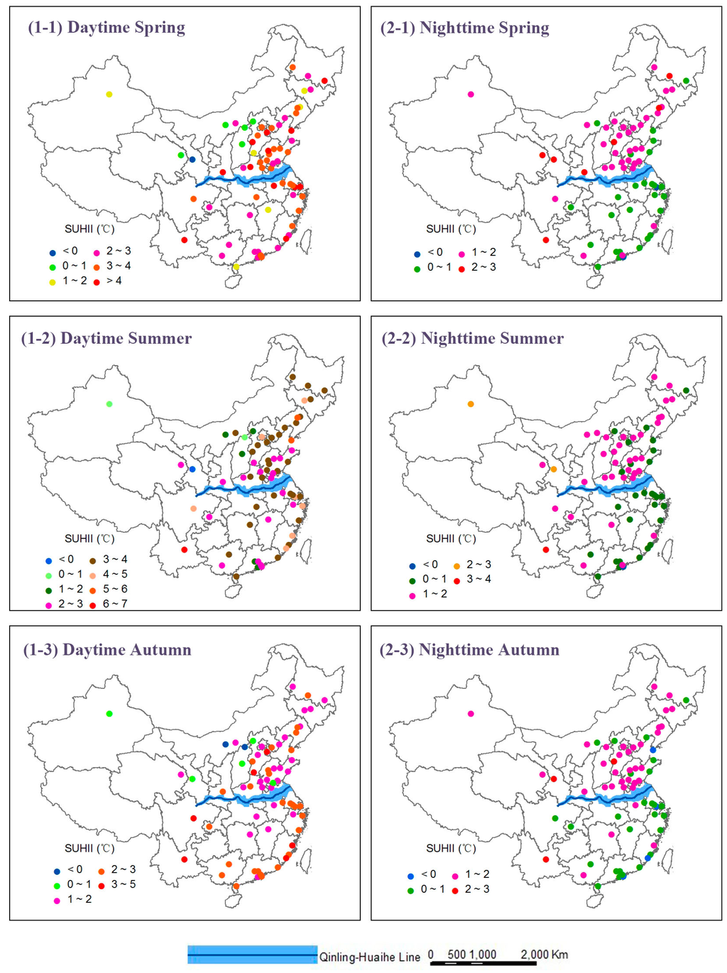
Figure 3. The spatial distribution of the seasonally and annually averaged SUHIIs during day time and night time from 2003 to 2010: (1-1) Daytime spring; (2-1) Nighttime Spring; (1-2) Daytime Summer; (2-2) Nighttime Summer; (1-3) Daytime Autumn; (2-3) Nighttime Autumn; (1-4) Daytime Winter; (2-4) Nighttime Winter; (1-5) Daytime Annual; (2-5) Nighttime Annual.

Figure 3. The spatial distribution of the seasonally and annually averaged SUHIIs during day time and night time from 2003 to 2010: (1-1) Daytime spring; (2-1) Nighttime Spring; (1-2) Daytime Summer; (2-2) Nighttime Summer; (1-3) Daytime Autumn; (2-3) Nighttime Autumn; (1-4) Daytime Winter; (2-4) Nighttime Winter; (1-5) Daytime Annual; (2-5) Nighttime Annual.

Table 2. Seasonally averaged values of SUHII and the variances over northern and southern China from 2003 to 2010 (Unit: K).

		Mean				Variance
		Spring	Summer	Autumn	Winter	Spring	Summer	Autumn	Winter
Daytime SUHII	Northern China	2.66	3.04	1.60	−0.62	1.28	0.25	0.62	1.88
	Southern China	3.61	4.35	3.23	1.87	0.28	0.70	0.24	0.37
Nighttime SUHII	Northern China	1.53	1.37	1.30	1.72	0.06	0.06	0.06	0.12
	Southern China	1.07	1.69	1.06	0.65	0.12	0.11	0.10	0.11

Table 2. Seasonally averaged values of SUHII and the variances over northern and southern China from 2003 to 2010 (Unit: K).

		Mean				Variance
		Spring	Summer	Autumn	Winter	Spring	Summer	Autumn	Winter
Daytime SUHII	Northern China	2.66	3.04	1.60	−0.62	1.28	0.25	0.62	1.88
	Southern China	3.61	4.35	3.23	1.87	0.28	0.70	0.24	0.37
Nighttime SUHII	Northern China	1.53	1.37	1.30	1.72	0.06	0.06	0.06	0.12
	Southern China	1.07	1.69	1.06	0.65	0.12	0.11	0.10	0.11

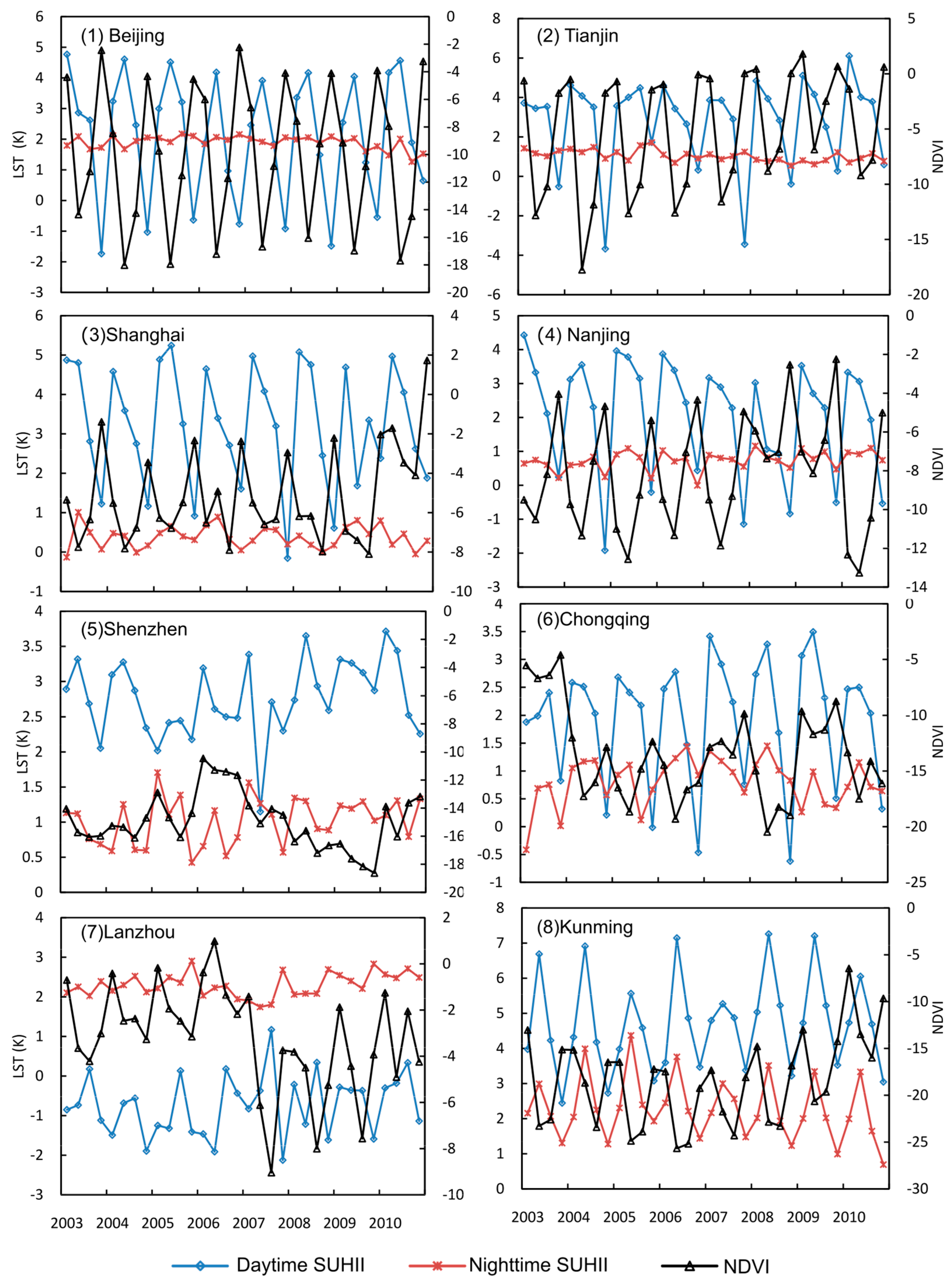
The different temporal patterns of SUHII over eight typical cities in China also exhibit theabove-mentioned differences (Figure 4). The largest daytime SUHII (more than 7 K) in summer occurred in Kunming. This resulted from the regional environment, especially the land cover types surrounding the urban area. Kunming is surrounded by mountains covered by dense and tall vegetation, which made the surrounding rural areas much cooler than the less-vegetated urban area [25]. In contrast, sparsely vegetated areas, such as the Gobi desert, have the ability to absorb solar energy and store it as heat, thus, lowering the temperature gradient between the urban and rural areas [49,50,51]. For example, in Lanzhou, the summer daytime SUHIIs were actually slightly negative (−1 K) during the study period. Six other typical cities also showed distinct and different diurnal and seasonal variation in the SUHIIs from north to south China (Figure 4). The SUHIIs exhibited quite similar temporal patterns in Beijing and Tianjin city, with stable nighttime SUHIIs and seasonal variation in the daytime SUHIIs. Shanghai, Nanjing, and Chongqing exhibited pronounced seasonal variation in both daytime and nighttime SUHII. For Shenzhen city, the frequency of nighttime SUHII fluctuation was high (Figure 4(5)).

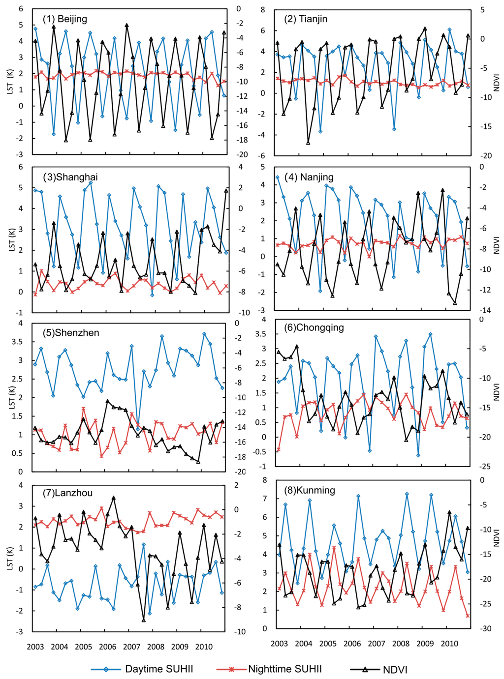
Figure 4. The seasonally averaged SUHII and NDVI from 2003 to 2010 for eight typical cities: (1) Beijing; (2) Tianjin; (3) Shanghai; (4) Nanjing; (5) Shenzhen; (6) Chongqing; (7) Lanzhou; (8) Kunming. The locations of these cities are shown in Figure 1.

Figure 4. The seasonally averaged SUHII and NDVI from 2003 to 2010 for eight typical cities: (1) Beijing; (2) Tianjin; (3) Shanghai; (4) Nanjing; (5) Shenzhen; (6) Chongqing; (7) Lanzhou; (8) Kunming. The locations of these cities are shown in Figure 1.

3.2. Evaluation of Rule-Based SUHII Models

Four rule-based SUHII models were established by taking the summer SUHIIs as the target variables. The results are described in Table 3. Each rule means that if the explanatory variables satisfy the conditions, the SUHII can be simulated using the corresponding expression.

Table 3. Sub-models for the rule-based SUHII simulation (Unit: K).

Model 1: For Daytime Summer SUHIIs of Cities Located in Northern China
Rule	Condition	SUHII Simulation
1	L3 > −5.014	SUHII = 3.0977 − 3.63 U3 + 0.606 L4 − 1.05 L1 − 0.32 L2 + 0.24 A6 − 0.017 L3 − 0.13 U2 + 0.12 A3 + 0.11 A2 + 0.4 U4
2	L3 ≤ −5.014, L4 > −0.414	SUHII = 0.7687 − 0.131 L3 + 0.37 L4 + 0.66 A6 − 0.75 U2 − 0.46 L2 + 0.56 U3 + 0.07 A4 + 0.11 A3 + 0.1 A2 + 0.2 U4
3	L3 ≤ −5.014, L4 ≤ −0.414	SUHII = 1.2153 − 1.64 L2 + 1.26 A4 − 0.154 L3 − 0.69 U2 + 0.52 U3 + 0.41 A1 − 0.39 A2 + 0.18 A6 + 0.026 L4 − 0.2 U4 + 0.11 U1
Model 2: For Daytime Summer SUHIIs of Cities Located in Southern China
Rule	Condition	SUHII Simulation
1	A4 ≤ 1.455, U1 > 1.019,U2 ≤ 0.554	SUHII = 2.091 + 0.82 A5 + 0.389 A6 − 0.3 L1 − 0.184 A3 − 0.13 U3
2	A4 > 1.455, U2 > 0.918	SUHII = −0.1925 + 2.14 U2 + 0.187 A3 − 0.3 L2 − 0.033 L3
3	A4 > 1.455,U2 ≤ 0.918	SUHII = 11.3059 − 2.36 U2 − 7.5 U4 − 0.694 A6− 0.4 L2 + 0.025 A3 − 0.004 L3
4	A4≤1.455, U1 > 1.019,U2 > 0.554	SUHII = 2.8774 + 1.35 A5 + 0.74 A4 + 0.642 A6 − 0.5 L1 − 0.304 A3 − 0.22 U3 − 0.2 U2
5	A4 ≤ 1.455, U1 ≤ 1.019, U2 > 0.400	SUHII = 1.8864 + 1.67 A5 + 2.42 U1 − 0.79 U2 − 0.32 L1 + 0.136 A2
6	A4 ≤ 1.455, U1 ≤ 1.019,U2 ≤ 0.400	SUHII = 59.7246 − 58.05 U4 − 7.58 U1 + 1.807 A4
Model 3: For Nighttime Summer SUHIIs of Cities Located in Northern China
Rule	Condition	SUHII Simulation
1	L4 > −0.035	SUHII = 0.8718 − 0.221 A5 + 0.315 L2 − 0.129 L4 + 0.31 U3
2	L4 ≤ −0.035, A5 ≤ 0.635	SUHII = 0.7287 − 0.208 L4 + 0.254 U2
3	L4 ≤ −0.035, A5 > 0.635	SUHII = 2.6139 + 0.526 A4 − 0.408 L2 − 0.129L4+0.325 U2 − 1.34 U4 − 0.134 A6 − 0.139 U3 + 0.0106 L3 − 0.103 A1
Model 4: For nighttime summer SUHIIs of Cities Located in Southern China
Rule	Condition	SUHII Simulation
1	L3 > −18.686, A1 > 0.954	SUHII = 0.1256 − 0.056 L3 − 0.18 U2 + 0.067 A1
2	L3 > −18.686, A1 ≤ 0.954	SUHII = 0.1653 + 1.304 A1 + 0.463 A5 − 0.416 L1 − 0.016 L3
3	L3 ≤ −18.686, U3 ≤ 0.4222	SUHII =−4.2273 + 13.297 U3 − 0.12 L3+ 0.356 A5 − 0.024 A3 + 0.011 L4
4	L3 ≤ −18.686, U3 > 0.422	SUHII = −2.5461 − 1.125 A3 − 0.236 L3 + 0.57 L4 + 0.74 A5 − 0.445 U3

A: anthropogenic heat discharge; L: land surface descriptors; U: urban form indicator. Detailed information about the indicators is listed in Table 1.

Table 3. Sub-models for the rule-based SUHII simulation (Unit: K).

Model 1: For Daytime Summer SUHIIs of Cities Located in Northern China
Rule	Condition	SUHII Simulation
1	L3 > −5.014	SUHII = 3.0977 − 3.63 U3 + 0.606 L4 − 1.05 L1 − 0.32 L2 + 0.24 A6 − 0.017 L3 − 0.13 U2 + 0.12 A3 + 0.11 A2 + 0.4 U4
2	L3 ≤ −5.014, L4 > −0.414	SUHII = 0.7687 − 0.131 L3 + 0.37 L4 + 0.66 A6 − 0.75 U2 − 0.46 L2 + 0.56 U3 + 0.07 A4 + 0.11 A3 + 0.1 A2 + 0.2 U4
3	L3 ≤ −5.014, L4 ≤ −0.414	SUHII = 1.2153 − 1.64 L2 + 1.26 A4 − 0.154 L3 − 0.69 U2 + 0.52 U3 + 0.41 A1 − 0.39 A2 + 0.18 A6 + 0.026 L4 − 0.2 U4 + 0.11 U1
Model 2: For Daytime Summer SUHIIs of Cities Located in Southern China
Rule	Condition	SUHII Simulation
1	A4 ≤ 1.455, U1 > 1.019,U2 ≤ 0.554	SUHII = 2.091 + 0.82 A5 + 0.389 A6 − 0.3 L1 − 0.184 A3 − 0.13 U3
2	A4 > 1.455, U2 > 0.918	SUHII = −0.1925 + 2.14 U2 + 0.187 A3 − 0.3 L2 − 0.033 L3
3	A4 > 1.455,U2 ≤ 0.918	SUHII = 11.3059 − 2.36 U2 − 7.5 U4 − 0.694 A6− 0.4 L2 + 0.025 A3 − 0.004 L3
4	A4≤1.455, U1 > 1.019,U2 > 0.554	SUHII = 2.8774 + 1.35 A5 + 0.74 A4 + 0.642 A6 − 0.5 L1 − 0.304 A3 − 0.22 U3 − 0.2 U2
5	A4 ≤ 1.455, U1 ≤ 1.019, U2 > 0.400	SUHII = 1.8864 + 1.67 A5 + 2.42 U1 − 0.79 U2 − 0.32 L1 + 0.136 A2
6	A4 ≤ 1.455, U1 ≤ 1.019,U2 ≤ 0.400	SUHII = 59.7246 − 58.05 U4 − 7.58 U1 + 1.807 A4
Model 3: For Nighttime Summer SUHIIs of Cities Located in Northern China
Rule	Condition	SUHII Simulation
1	L4 > −0.035	SUHII = 0.8718 − 0.221 A5 + 0.315 L2 − 0.129 L4 + 0.31 U3
2	L4 ≤ −0.035, A5 ≤ 0.635	SUHII = 0.7287 − 0.208 L4 + 0.254 U2
3	L4 ≤ −0.035, A5 > 0.635	SUHII = 2.6139 + 0.526 A4 − 0.408 L2 − 0.129L4+0.325 U2 − 1.34 U4 − 0.134 A6 − 0.139 U3 + 0.0106 L3 − 0.103 A1
Model 4: For nighttime summer SUHIIs of Cities Located in Southern China
Rule	Condition	SUHII Simulation
1	L3 > −18.686, A1 > 0.954	SUHII = 0.1256 − 0.056 L3 − 0.18 U2 + 0.067 A1
2	L3 > −18.686, A1 ≤ 0.954	SUHII = 0.1653 + 1.304 A1 + 0.463 A5 − 0.416 L1 − 0.016 L3
3	L3 ≤ −18.686, U3 ≤ 0.4222	SUHII =−4.2273 + 13.297 U3 − 0.12 L3+ 0.356 A5 − 0.024 A3 + 0.011 L4
4	L3 ≤ −18.686, U3 > 0.422	SUHII = −2.5461 − 1.125 A3 − 0.236 L3 + 0.57 L4 + 0.74 A5 − 0.445 U3

A: anthropogenic heat discharge; L: land surface descriptors; U: urban form indicator. Detailed information about the indicators is listed in Table 1.

The performance of each model was evaluated based on AE, RE, CC and the RMSE (Table 4). All four models were significant at the 0.001 level, with small AEs (0.57, 0.79, 0.25, 0.23, respectively), small REs (0.58, 0.82, 0.65, 0.52, respectively), significant CCs (0.84, 0.63, 0.80, 0.91, respectively) and small RMSEs (0.74, 1.32, 0.37, 0.46, respectively). These models were also validated by comparing the simulated SUHIIs with the observed SUHIIs during 2009 and 2010 (Figure 5). All four scatter plots were close to the 1:1 line. The two models for the nighttime SUHIIs were more precise, with the R² equal to 0.510 in northern China (Model 3) and 0.602 in southern China (Model 4). The model for the daytime SUHIIs in northern China was also significant with an R² equal to 0.592. However, the model for the daytime SUHII in southern China (Model 2) had a relatively small R² (0.308) value and a larger RMSE value (1.32 K), which was affected by the extreme temperature in the city of Kunming.

Table 4. Accuracy statistics for each SUHII model.AE: average error; RE: relative error; CC: correlation coefficient; RMSE: root mean square error.

Model	AE	RE	CC	RMSE
1: daytime summer SUHIIs in northern China	0.57	0.58	0.84	0.74
2: daytime summer SUHIIs in southern China	0.79	0.82	0.63	1.32
3: nighttime summer SUHIIs in northern China	0.25	0.65	0.80	0.37
4: nighttime summer SUHIIs in southern China	0.23	0.52	0.91	0.46

Table 4. Accuracy statistics for each SUHII model.AE: average error; RE: relative error; CC: correlation coefficient; RMSE: root mean square error.

Model	AE	RE	CC	RMSE
1: daytime summer SUHIIs in northern China	0.57	0.58	0.84	0.74
2: daytime summer SUHIIs in southern China	0.79	0.82	0.63	1.32
3: nighttime summer SUHIIs in northern China	0.25	0.65	0.80	0.37
4: nighttime summer SUHIIs in southern China	0.23	0.52	0.91	0.46

Figure 5. Scatterplots between the observed SUHIIs from the MODIS datasets and the simulated SUHIIs for model: (1) daytime summer SUHIIs in northern China; (2) daytime summer SUHIIs in southern China; (3) nighttime summer SUHIIs in northern China; (4) nighttime summer SUHIIs in southern China. The scatter plots were based on the test set in 2009 and 2010 and, thus, two points for the same city are shown in the figure.

Figure 5. Scatterplots between the observed SUHIIs from the MODIS datasets and the simulated SUHIIs for model: (1) daytime summer SUHIIs in northern China; (2) daytime summer SUHIIs in southern China; (3) nighttime summer SUHIIs in northern China; (4) nighttime summer SUHIIs in southern China. The scatter plots were based on the test set in 2009 and 2010 and, thus, two points for the same city are shown in the figure.

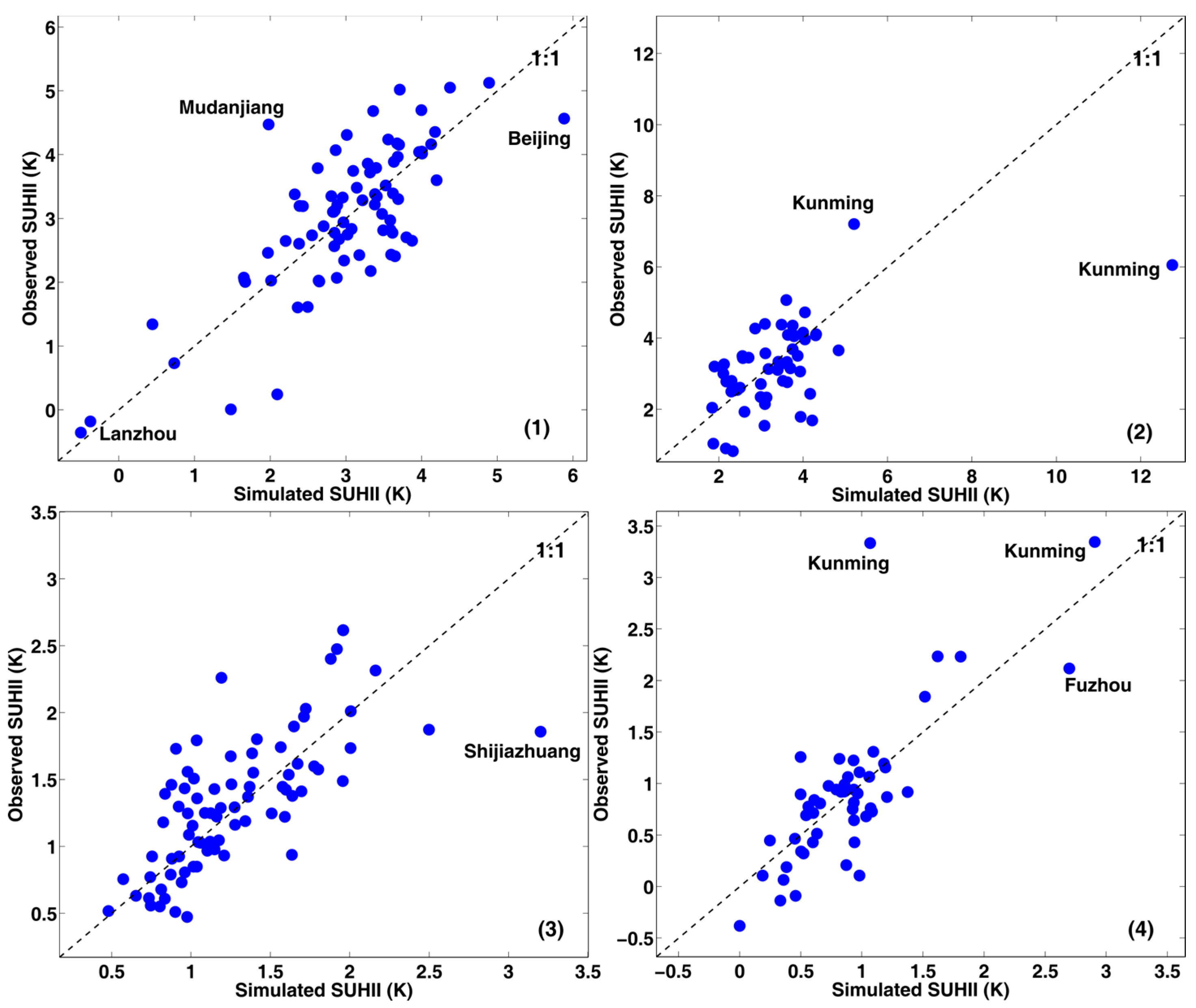
The models simulated the SUHIIs fairly well at the city level. They captured exceptional SUHII values for some sites, such as the extremely large SUHII in Kunming and Fuzhou and the extremely small SUHII in Lanzhou (Figure 5). However, the models also slightly under-estimated or over-estimated the SUHIIs for some cities. Significant under-estimation occurred for cities such as Mudanjiang, while significant over-estimation occurred for cities such as Beijing and Shijiazhuang. Generally, the accuracy of the models was acceptable, given the complex interactions in the urban system.

3.3. The Importance of Each Factor to SUHII

The relative importance of each factor was measured by a linear combination of its usage in the rule conditions and the simulation expressions, with 100 indicating the greatest possible contribution and 0 the least contribution. The importance of each factor is shown in Table 5. Although all the selected explanatory variables were related to SUHII, their contributions varied. Specifically, for summer daytime SUHIIs in northern China (Model 1), the two most important input variables were the ΔNDVI (L3) and Δalbedo (L4). For summer daytime SUHIIs in southern China (Model 2), the number of public buses (A4) and population density (U2) were the most important factors. For summer nighttime SUHIIs in northern China (Model 3), the two most important variables were the number of taxis (A5) and Δalbedo (L4). For nighttime summer SUHII in southern China (Model 4), ΔNDVI (L3) and annual electricity consumption (A1) were the major factors. The variables with the greatest influence on SUHII were land surface characteristics (e.g., ΔNDVI and Δalbedo). Anthropogenic heat discharge was associated with SUHII in southern China, where the number of public buses and annual electricity consumption were the second most important factors in Model 2and Model 4. The urban form descriptors (except population density) were relatively less important, especially in southern China.

Table 5. Importance of input variables for each model. Note: Detailed information on Models 1–4 is listed in Table 3. The number indicates the relative importance of each factor to SUHII, with 100 being the largest possible score and 0 the smallest score. The bold font indicates the two most important factors.

Code	Name of Indicator	Model 1	Model 2	Model 3	Model 4
A1	Annual electricity consumption	24.5	0	17.0	84.0
A2	LPG gas supply	50.0	15.5	0	0
A3	Annual water consumption	25.5	32.0	0	8.0
A4	Number of public buses	45.0	64.0	17.0	0
A5	Number of taxis	0	31.0	50.0	27.5
A6	GDP of the built-up area	50.0	23.0	17.0	0
L1	Road area at the end of the year	5.0	31.0	0	19.5
L2	Size of built-up area	50	16.5	32.5	0
L3	ΔNDVI	100.0	16.5	17.0	100.0
L4	Δalbedo	95.0	0	100.0	8.0
U1	Green area of built-up area	24.5	51.5	0	0
U2	Population density	50.0	93.5	34.5	22.5
U3	Construction area coverage	50.0	15.5	32.5	16.0
U4	Compactness	50.0	10.0	17.0	0

Table 5. Importance of input variables for each model. Note: Detailed information on Models 1–4 is listed in Table 3. The number indicates the relative importance of each factor to SUHII, with 100 being the largest possible score and 0 the smallest score. The bold font indicates the two most important factors.

Code	Name of Indicator	Model 1	Model 2	Model 3	Model 4
A1	Annual electricity consumption	24.5	0	17.0	84.0
A2	LPG gas supply	50.0	15.5	0	0
A3	Annual water consumption	25.5	32.0	0	8.0
A4	Number of public buses	45.0	64.0	17.0	0
A5	Number of taxis	0	31.0	50.0	27.5
A6	GDP of the built-up area	50.0	23.0	17.0	0
L1	Road area at the end of the year	5.0	31.0	0	19.5
L2	Size of built-up area	50	16.5	32.5	0
L3	ΔNDVI	100.0	16.5	17.0	100.0
L4	Δalbedo	95.0	0	100.0	8.0
U1	Green area of built-up area	24.5	51.5	0	0
U2	Population density	50.0	93.5	34.5	22.5
U3	Construction area coverage	50.0	15.5	32.5	16.0
U4	Compactness	50.0	10.0	17.0	0

4. Discussion

4.1. Theoretical and Practical Implications

The distinct SUHI and the seasonal variation for the daytime SUHII observed in this research are consistent with previous studies. This research indicated that the daytime SUHIIs were greater than the nighttime SUHIIs except in winter in northern China. Previous reports have also documented that in the daytime the urban-rural contrast in surface temperature is often much larger than the difference in air temperature [52,53], and this research was focused on the SUHI defined from surface thermal radiance. There were also reports indicating that the SUHII was more significant during the night time [54].This discrepancy may be related to issues of temporal scale. On the one hand, SUHIs in different seasons have different diurnal patterns [52,55,56]. On the other, the averaged LST of the different time periods used may introduce bias. Peng et al. [27] reported larger annually averaged daytime SUHIIs, which is consistent with this research based on the seasonally averaged SUHII. Those studies that reported larger nighttime SUHIIs were often conducted based on a single day [54]. Therefore, we infer that the diurnal variation in the SUHII is seasonally varied.

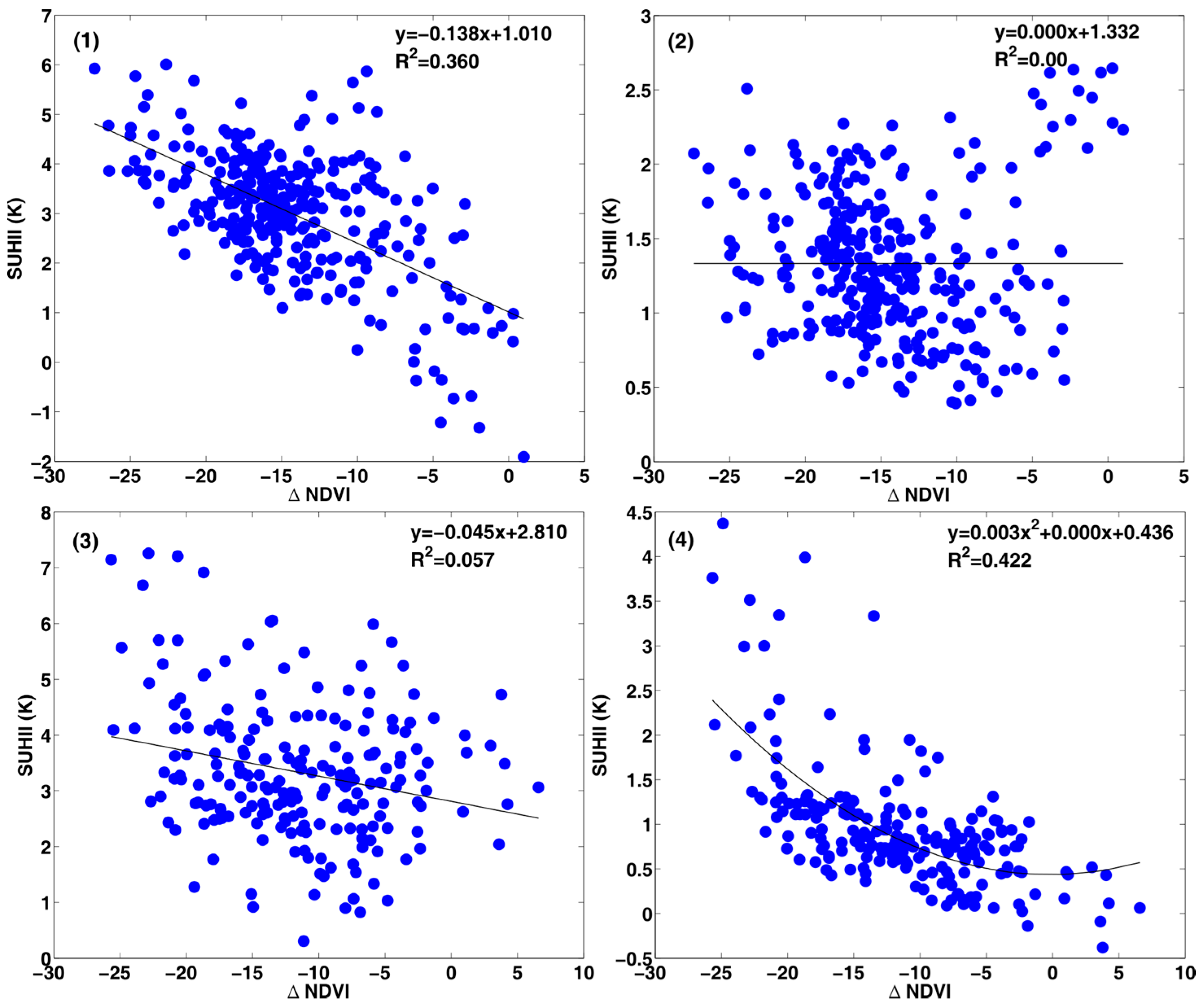
The relationship between the SUHII and NDVI depends on the location of the cities and the time of year, which implies that increasing vegetation coverage is not always effective in mitigating the SUHI effect. The relationships between summer SUHII (daytime and nighttime) and ΔNDVI (northern China and southern China) are shown in Figure 6. For the daytime SUHII in southern China, the contribution of NDVI was relatively small. This may be partly due to the abundant tree cover in southern China at present and so it is not thought to be a limiting factor. In northern China, the daytime SUHIIs were significantly negatively correlated with ΔNDVI (R² = 0.36), which suggests that increasing vegetation coverage may be a viable option in northern China for mitigating the daytime UHI effect.

The effects of anthropogenic heat discharge on the SUHI were not significant. This is likely to be because the anthropogenic heat discharge influences mainly the near surface UHI, not the surface UHI, but also because of issues of spatial scale. Several causes of the UHI have been documented and the influence of each may vary with spatial measurement scale [57]. For example, the regional geographic environment and weather conditions are important in meso-scale UHI studies, but they can be negligible in micro-scale UHI studies. On the contrary, anthropogenic heat release may be an important variable in building-scale UHI studies, while it may be insignificant in meso-scale UHI studies. As the SUHI was simulated at the regional scale in this research, it is expected that the influence of anthropogenic heat discharge may be minor. Nevertheless, the second most important factors in southern China were found to be annual electricity consumption and the number of taxis. While these results are interesting, they reveal only an association with SUHII and do not imply cause and effect. Thus, it does not necessarily follow that reducing the number of cars or electricity consumption will reduce SUHII.

The three parameters describing urban form (compactness, porosity, density) in this research have a complex contribution to SUHIs. Population density (U2) has relatively greater importance than compactness and porosity. The significant relationship between LST and population has also been found in the literature [58]. However, no quantitative studies have been published on the role of the other two dimensions of urban form on SUHII. Here, the small contribution of porosity and compactness to the SUHI on the regional scale was indicated by the relatively low importance of green-areas within built-up areas (U1), construction area coverage (U3) and compactness (U4), especially in southern China. These results provide further evidence on the potential environmental benefit of “the compact city”, which is a well debated issue [43]. This research indicated that at the regional scale compactness and porosity have no significant effect on SUHII. This may be explained by the multifaceted impact of the compact city. On the one hand, a compact city may have more developed urban infrastructure and land utilization, as the distance between the various parts of the inner city are shortened. The dependence of citizens on cars would also be reduced and this would lead to lower pollutant emissions and energy consumption. On the other hand, the concentrated structure of a compact city may also be in conflict with the development of green cities, which may mitigate the UHI effect. Therefore, the concept of the compact city and its potential environmental benefits requires further research based on the study of single cities using more detailed datasets including fine spatial resolution images.

Figure 6. Relationship between summer SUHII and ΔNDVI for: (1) daytime SUHII in northern China; (2) daytime SUHII in southern China; (3) nighttime SUHII in northern China; and (4) nighttime SUHII in southern China.

Figure 6. Relationship between summer SUHII and ΔNDVI for: (1) daytime SUHII in northern China; (2) daytime SUHII in southern China; (3) nighttime SUHII in northern China; and (4) nighttime SUHII in southern China.

4.2. Limitations

Several limitations of this research can be identified. Firstly, although the DMSP/OLS nighttime lights images were the optimal choice for extracting urban areas at a regional and national scale, the over-glow effect may affect the spatiotemporal patterns of the SUHI. The “rural” surfaces defined as the buffering zones of the urban area may also introduce bias. Future studies should use fine spatial resolution land use/land cover data to identify urban and rural areas using representative land cover types. Secondly, when fitting the regression tree models, the dates of the target variable (SUHII) derived from the MODIS products were not perfectly congruent with the temporal range of the explanatory variables from the statistical yearbooks. More specifically, we used summer averaged SUHII as the target variable, while the explanatory variables were based on demographic data for the whole year. Although the statistical data at the end of the year from statistical yearbooks represented adequately the heat discharge intensities between cities and years, they unavoidably reduced the explanatory power of the model. Thirdly, while every effort was made to provide a comprehensive list of explanatory factors, ultimately only the most controllable and available variables were included. Other factors that may influence SUHII, such as topography, soil moisture, complexity and centrality, could not be assembled on a national scale and, thus, were not considered in this research. Further studies should use fine spatiotemporal resolution datasets (e.g., basic geographic information and land use/land cover data) to explore their effects on SUHII in specific typical cities.

5. Conclusions

This research provided a new approach to studying the SUHI. By gathering multi-source remote sensing images and demographic data, this research compared the spatiotemporal patterns of SUHIIs and assessed specific related factors in major Chinese cities using regression tree models. The patterns of SUHII observed and their relation with explanatory factors were found to be both spatially and temporally varying in northern and southern China. The results have important theoretical significance and are of use to urban planners who should consider taking mitigation measures in relation to the UHI effect.

Significant SUHII differences were observed temporally (daytime and nighttime) and spatially (northern China and southern China) in the 67 major Chinese cities studied. Daytime SUHII exhibited seasonal variation across China, with the largest SUHII in summer and smallest SUHII in winter. The diurnal patterns in SUHII varied seasonally. Southern China experienced much larger and more stable daytime SUHIIs than northern China during the study period. The nighttime SUHIIs in northern China were larger and more stable than those in southern China.

The factors associated with SUHII varied between northern and southern China. In northern China, the daytime SUHII was significantly correlated with ΔNDVI, which suggests that increasing vegetation coverage may be an effective way to mitigate the UHI effect in northern China. In southern China, anthropogenic heat discharge was relatively more important, with annual electricity consumption (A1) and number of public buses (A4) obtaining the second highest score.

References

- Grimm, N.B.; Faeth, S.H.; Golubiewski, N.E.; Redman, C.L.; Wu, J.G.; Bai, X.M.; Briggs, J.M. Global change and the ecology of cities. Science 2008, 319, 756–760. [Google Scholar] [CrossRef] [PubMed]
- Oke, T.R. The energetic basis of the urban heat island. Q. J. Roy. Meteor. Soc. 1982, 108, 1–24. [Google Scholar]
- Voogt, J.A. Urban Heat Islands: Hotter Cities. Available online: http://www.actionbioscience.org/environment/voogt.html (accessed on 29 January 2015).
- Bohnenstengel, S.I.; Evans, S.; Clark, P.A.; Belcher, S.E. Simulations of the london urban heat island. Q. J. Roy. Meteor. Soc. 2011, 137, 1625–1640. [Google Scholar] [CrossRef]
- Pal, S.; Xueref-Remy, I.; Ammoura, L.; Chazette, P.; Gibert, F.; Royer, P.; Dieudonné, E.; Dupont, J.C.; Haeffelin, M.; Lac, C.; et al. Spatio-temporal variability of the atmospheric boundary layer depth over the paris agglomeration: An assessment of the impact of the urban heat island intensity. Atmos. Environ. 2012, 63, 261–275. [Google Scholar] [CrossRef]
- Santamouris, M.; Papanikolaou, N.; Livada, I.; Koronakis, I.; Georgakis, C.; Argiriou, A.; Assimakopoulos, D.N. On the impact of urban climate on the energy consumption of buildings. Sol. Energy 2001, 70, 201–216. [Google Scholar] [CrossRef]
- Epstein, P.R. Climate change and human health. New Engl. J. Med. 2005, 353, 1433–1436. [Google Scholar] [CrossRef] [PubMed]
- Sarrat, C.; Lemonsu, A.; Masson, V.; Guedalia, D. Impact of urban heat island on regional atmospheric pollution. Atmos. Environ. 2006, 40, 1743–1758. [Google Scholar] [CrossRef]
- Pal, S.; Devara, P.C.S. A wavelet-based spectral analysis of long-term time series of optical properties of aerosols obtained by LiDAR and radiometer measurements over an urban station in western India. J. Atmos. Sol. Terr. Phys. 2012, 84–85, 75–87. [Google Scholar] [CrossRef]
- Lac, C.; Donnelly, R.P.; Masson, V.; Pal, S.; Riette, S.; Donier, S.; Queguiner, S.; Tanguy, G.; Ammoura, L.; Xueref-Remy, I. CO2 dispersion modelling over Paris region within the CO2-MEGAPARIS project. Atmos. Chem. Phys. 2013, 13, 4941–4961. [Google Scholar] [CrossRef]
- Owen, T.W.; Carlson, T.N.; Gillies, R.R. An assessment of satellite remotely-sensed land cover parameters in quantitatively describing the climatic effect of urbanization. Int. J. Remote Sens. 1998, 19, 1663–1681. [Google Scholar] [CrossRef]
- Streutker, D.R. Satellite-measured growth of the urban heat island of Houston, Texas. Remote Sens. Environ. 2003, 85, 282–289. [Google Scholar] [CrossRef]
- Voogt, J.A.; Oke, T.R. Thermal remote sensing of urban climates. Remote Sens. Environ. 2003, 86, 370–384. [Google Scholar] [CrossRef]
- Patino, J.E.; Duque, J.C. A review of regional science applications of satellite remote sensing in urban settings. Comput. Environ. Urban 2013, 37, 1–17. [Google Scholar] [CrossRef]
- Huang, B.; Wang, J.; Song, H.; Fu, D.; Wong, K. Generating high spatiotemporal resolution land surface temperature for urban heat island monitoring. IEEE Trans. Geosci. Remote Sens. Lett. 2013, 10, 1011–1015. [Google Scholar] [CrossRef]
- Weng, Q.H. Thermal infrared remote sensing for urban climate and environmental studies: Methods, applications, and trends. ISPRSJ. Photogramm. Remote Sens. 2009, 64, 335–344. [Google Scholar] [CrossRef]
- Xiao, R.B.; Weng, Q.H.; Ouyang, Z.Y.; Li, W.F.; Schienke, E.W.; Zhang, Z.M. Land surface temperature variation and major factors in Beijing, China. Photogramm. Eng. Remote Sens. 2008, 74, 451–461. [Google Scholar] [CrossRef]
- Li, J.; Wang, X.; Wang, X.; Ma, W.; Zhang, H. Remote sensing evaluation of urban heat island and its spatial pattern of the Shanghai metropolitan area, China. Ecol. Complex. 2009, 6, 413–420. [Google Scholar] [CrossRef]
- Amiri, R.; Weng, Q.; Alimohammadi, A.; Alavipanah, S.K. Spatial-temporal dynamics of land surface temperature in relation to fractional vegetation cover and land use/cover in the Tabriz urban area, Iran. Remote Sens. Environ. 2009, 113, 2606–2617. [Google Scholar] [CrossRef]
- Chen, X.-L.; Zhao, H.-M.; Li, P.-X.; Yin, Z.-Y. Remote sensing image-based analysis of the relationship between urban heat island and land use/cover changes. Remote Sens. Environ. 2006, 104, 133–146. [Google Scholar] [CrossRef]
- Su, Y.; Foody, G.M.; Cheng, K. Spatial non-stationarity in the relationships between land cover and surface temperature in an urban heat island and its impacts on thermally sensitive populations. Landscape Urban Plan. 2012, 107, 172–180. [Google Scholar] [CrossRef]
- Weng, Q.H.; Lu, D.S.; Schubring, J. Estimation of land surface temperature-vegetation abundance relationship for urban heat island studies. Remote Sens. Environ. 2004, 89, 467–483. [Google Scholar] [CrossRef]
- Fan, H.; Sailor, D.J. Modeling the impacts of anthropogenic heating on the urban climate of Philadelphia: A comparison of implementations in two PBL schemes. Atmos. Environ. 2005, 39, 73–84. [Google Scholar] [CrossRef]
- Tran, H.; Uchihama, D.; Ochi, S.; Yasuoka, Y. Assessment with satellite data of the urban heat island effects in Asian Mega cities. Int. J. Appl. Earth Obs. Geoinf. 2006, 8, 34–48. [Google Scholar] [CrossRef]
- Imhoff, M.L.; Zhang, P.; Wolfe, R.E.; Bounoua, L. Remote sensing of the urban heat island effect across biomes in the continental USA. Remote Sens. Environ. 2010, 114, 504–513. [Google Scholar] [CrossRef]
- Pongrácz, R.; Bartholy, J.; Dezső, Z. Application of remotely sensed thermal information to urban climatology of central European cities. Phys. Chem. Earth 2010, 35, 95–99. [Google Scholar] [CrossRef]
- Peng, S.; Piao, S.; Ciais, P.; Friedlingstein, P.; Ottle, C.; Bréon, F.O.-M.; Nan, H.; Zhou, L.; Myneni, R.B. Surface urban heat island across 419 global big cities. Environ. Sci. Tech. 2011, 46, 696–703. [Google Scholar] [CrossRef]
- Holling, C.S. Understanding the complexity of economic, ecological, and social systems. Ecosystems 2001, 4, 390–405. [Google Scholar] [CrossRef]
- Li, B. Why is the holistic approach becoming so important in landscape ecology? Landscape Urban Plan. 2000, 50, 27–41. [Google Scholar] [CrossRef]
- Huang, J.L.; Wang, R.S.; Shi, Y. Urban climate change: A comprehensive ecological analysis of the thermo-effects of major Chinese cities. Ecol. Complex. 2010, 7, 188–197. [Google Scholar] [CrossRef]
- Long, Y.; Mao, Q.Z.; Yang, D.F.; Wang, J.W. A multi-agent model for urban form, transportation energy consumption and environmental impact integrated simulation. Acta Geogr. Sinica 2011, 66, 1033–1044. [Google Scholar]
- Liu, M.L.; Tian, H.Q. China’s land cover and land use change from 1700 to 2005: Estimations from high-resolution satellite data and historical archives. Glob. Biogeochem. Cy. 2010, 24. [Google Scholar] [CrossRef]
- Zhou, L.M.; Dickinson, R.E.; Tian, Y.H.; Fang, J.Y.; Li, Q.X.; Kaufmann, R.K.; Tucker, C.J.; Myneni, R.B. Evidence for a significant urbanization effect on climate in China. Proc. Natl. Acad. Sci. USA 2004, 101, 9540–9544. [Google Scholar] [CrossRef] [PubMed]
- Li, Q.; Zhang, H.; Liu, X.; Huang, J. Urban heat island effect on annual mean temperature during the last 50 years in China. Theor. Appl. Climatol. 2004, 79, 165–174. [Google Scholar] [CrossRef]
- The Geonames Geographical Database. Available online: Http://www.geonames.org/ (accessed on 20 March 2015).
- Zheng, D. Eco-Geographical Regions in China; Commercial Press: Beijing, China, 2008. [Google Scholar]
- NASA’S Earth Observing System Data and Information System. Available online: Http://reverb.Echo.Nasa.Gov/reverb/ (accessed on 20 March 2015).
- National Geophysical Data Center/Earth Observation Group. Available online: Http://ngdc.noaa.gov/eog/ (accessed on 20 March 2015).
- Ma, T.; Zhou, C.; Pei, T.; Haynie, S.; Fan, J. Quantitative estimation of urbanization dynamics using time series of DMSP/OLS nighttime light data: A comparative case study from China’s cities. Remote Sens. Environ. 2012, 124, 99–107. [Google Scholar] [CrossRef]
- Oke, T.R. City size and the urban heat island. Atmos. Environ. 1973, 7, 769–779. [Google Scholar] [CrossRef]
- Imhoff, M.L.; Lawrence, W.T.; Stutzer, D.C.; Elvidge, C.D. A technique for using composite DMSP/OLS “city lights” satellite data to map urban area. Remote Sens. Environ. 1997, 61, 361–370. [Google Scholar] [CrossRef]
- Galster, G.; Hanson, R.; Ratcliffe, M.R.; Wolman, H.; Coleman, S.; Freihage, J. Wrestling sprawl to the ground: Defining and measuring an elusive concept. Hous. Policy Debate 2001, 12, 681–717. [Google Scholar] [CrossRef]
- Tsai, Y.H. Quantifying urban form: Compactness versus“sprawl”. Urban Stud. 2005, 42, 141–161. [Google Scholar] [CrossRef]
- Huang, J.; Lu, X.X.; Sellers, J.M. A global comparative analysis of urban form: Applying spatial metrics and remote sensing. Landscape Urban Plan. 2007, 82, 184–197. [Google Scholar] [CrossRef]
- Liu, J.; Wang, X.S.; Zhuang, D.F.; Zhang, W.; Hu, W.Y. Application of conves hull in identiftying the types of urban land expansion. Acta Geogr. Sinica 2003, 58, 885–892. [Google Scholar]
- Xiao, J.F.; Zhuang, Q.L.; Baldocchi, D.D.; Law, B.E.; Richardson, A.D.; Chen, J.Q.; Oren, R.; Starr, G.; Noormets, A.; Ma, S.Y.; et al. Estimation of net ecosystem carbon exchange for the conterminous united states by combining MODIS and AmeriFlux data. Agr. Forest Meteorol. 2008, 148, 1827–1847. [Google Scholar] [CrossRef]
- Yang, L.M.; Huang, C.Q.; Homer, C.G.; Wylie, B.K.; Coan, M.J. An approach for mapping large-area impervious surfaces: Synergistic use of Landsat-7 ETM+ and high spatial resolution imagery. Can. J. Remote Sens. 2003, 29, 230–240. [Google Scholar] [CrossRef]
- Yang, L.M.; Xian, G.; Klaver, J.M.; Deal, B. Urban land-cover change detection through sub-pixel imperviousness mapping using remotely sensed data. Photogramm. Eng. Remote Sens. 2003, 69, 1003–1010. [Google Scholar] [CrossRef]
- Bounoua, L.; Safia, A.; Masek, J.; Peters-Lidard, C.; Imhoff, M.L. Impact of urban growth on surface climate: A case study in Oran, Algeria. J. Appl. Meteorol. Clim. 2009, 48, 217–231. [Google Scholar] [CrossRef]
- Shephard, J.M. A review of current investigations of urban-induced rainfall and recommmendations for the future. Earth Interact. 2005, 9, 1–27. [Google Scholar] [CrossRef]
- Shepherd, J.M. Evidence of urban-induced precipitation variability in arid climate regimes. J. Arid Environ. 2006, 67, 607–628. [Google Scholar] [CrossRef]
- Cui, Y.Y.; de Foy, B. Seasonal variations of the urban heat island at the surface and the near-surface and reductions due to urban vegetation in Mexico city. J. Appl. Meteorol. Clim. 2012, 51, 855–868. [Google Scholar] [CrossRef]
- Voogt, J.A.; Oke, T.R. Complete urban surface temperatures. J. Appl. Meteorol. 1997, 36, 1117–1132. [Google Scholar] [CrossRef]
- Liu, L.; Zhang, Y. Urban heat island analysis using the landsat TM data and ASTER data: A case study in Hong Kong. Remote Sens. 2011, 3, 1535–1552. [Google Scholar] [CrossRef]
- Wang, K.; Wang, J.; Wang, P.; Sparrow, M.; Yang, J.; Chen, H. Influences of urbanization on surface characteristics as derived from the moderate-resolution imaging spectroradiometer: A case study for the Beijing metropolitan area. J. Geophys. Res.: Atmos. 2007, 112. [Google Scholar] [CrossRef]
- Bornstein, R.; Styrbicki-Imamura, R.; González, J.E.; Lebassi, B.; Fernando, H.J.S.; Klaić, Z.; McCulley, J.L. Interactions of global-warming and urban heat islands in different climate-zones. In National Security and Human Health Implications of Climate Change; Springer: Berlin, Germany, 2012; pp. 49–60. [Google Scholar]
- Mirzaei, P.A.; Haghighat, F. Approaches to study urban heat island—Abilities and limitations. Build. Environ. 2010, 45, 2192–2201. [Google Scholar] [CrossRef]
- Zhang, H.; Qi, Z.; Ye, X.; Cai, Y.; Ma, W.; Chen, M. Analysis of land use/land cover change, population shift, and their effects on spatiotemporal patterns of urban heat islands in metropolitan Shanghai, China. Appl. Geogr. 2013, 44, 121–133. [Google Scholar] [CrossRef]
© 2015 by the authors; licensee MDPI, Basel, Switzerland. This article is an open access article distributed under the terms and conditions of the Creative Commons Attribution license (http://creativecommons.org/licenses/by/4.0/).