Mapping Intra-Field Yield Variation Using High Resolution Satellite Imagery to Integrate Bioenergy and Environmental Stewardship in an Agricultural Watershed

Abstract

Biofuels are important alternatives for meeting our future energy needs. Successful bioenergy crop production requires maintaining environmental sustainability and minimum impacts on current net annual food, feed, and fiber production. The objectives of this study were to: (1) determine under-productive areas within an agricultural field in a watershed using a single date; high resolution remote sensing and (2) examine impacts of growing bioenergy crops in the under-productive areas using hydrologic modeling in order to facilitate sustainable landscape design. Normalized difference indices (NDIs) were computed based on the ratio of all possible two-band combinations using the RapidEye and the National Agricultural Imagery Program images collected in summer 2011. A multiple regression analysis was performed using 10 NDIs and five RapidEye spectral bands. The regression analysis suggested that the red and near infrared bands and NDI using red-edge and near infrared that is known as the red-edge normalized difference vegetation index (RENDVI) had the highest correlation (R² = 0.524) with the reference yield. Although predictive yield map showed striking similarity to the reference yield map, the model had modest correlation; thus, further research is needed to improve predictive capability for absolute yields. Forecasted impact using the Soil and Water Assessment Tool model of growing switchgrass (Panicum virgatum) on under-productive areas based on corn yield thresholds of 3.1, 4.7, and 6.3 Mg·ha⁻¹ showed reduction of tile NO₃-N and sediment exports by 15.9%–25.9% and 25%–39%, respectively. Corresponding reductions in water yields ranged from 0.9% to 2.5%. While further research is warranted, the study demonstrated the integration of remote sensing and hydrologic modeling to quantify the multifunctional value of projected future landscape patterns in a context of sustainable bioenergy crop production.

1. Introduction

Higher corn grain yields due to the expansion of production acreage and to better production efficiencies have led to an increase in availability of corn stover as a readily available feedstock for cellulosic biofuels. Corn stover consists of leaves and stalks of a corn plant (Zea mays L.) left in the field after grain harvesting. However, there are constraints on how much corn stover can be removed without negatively impacting subsequent soil productivity [1,2,3,4,5]. For example, Thompson and Tyner [6] used a linear programming model to project that at a price of about $66 per metric ton of corn stover, land use in the U.S. Midwest could shift from about 12% to 35% continuous corn. Such cost and farmer supply response projections would lead to more fertilizer use because of the nutrient requirements of a continuous corn agricultural system. The majority of current nutrient contributions to the Gulf of Mexico hypoxic zones is indeed fertilizer application in Midwestern agricultural systems (≈1500–3100 kg·N·km⁻²·year⁻¹) [7,8,9]. The U.S. Department of Agriculture (USDA), the U.S. Department of Energy (DOE), and the U.S. Environmental Protection Agency (EPA) also project cellulosic bioenergy crops such as perennial grasses as important components of the U.S. biomass feedstock portfolio, even in the U.S. Corn Belt [10].

The interest and focus on perennial herbaceous grasses for cellulosic bioenergy feedstock is due to the accrued beneficial impacts on the environment and ecosystem biodiversity as integral components of sustainable biomass. However, the integration of cellulosic bioenergy crops into existing agricultural systems requires a design approach that enhances environmental sustainability and minimally affects current net annual food, feed, and fiber production to trigger indirect land use change (iLUC). One option explored at plot and field scales is the use of marginal agricultural lands [11,12,13,14]. Definitions of marginal agricultural lands include sub-optimal production areas for commodity crops [14,15,16,17,18], areas susceptible to environmental degradation (e.g., erosion and nitrate leaching) when put into agricultural production [15,16], and small or irregular fields that are not suited for optimal farm machinery operations (based on discussions with farmers). Intra-field sub-optimal production areas are economically burdensome for farmers and may coincide with nutrient sink hotspots [19] and are therefore ideal for the integration of bioenergy crops into current agricultural systems to support sustainable landscapes and the provisioning of ecosystem services. Other potential uses of marginal lands not explored in this manuscript include sites for solar panels or wind turbines. However, patches of marginal lands are likely too small for those types of energy development.

Remote sensing is a reliable and cost-effective method to forecast crop yields over large areas based on the optical properties of crops such as chlorophyll absorption and mesophyll structure of foliage [20,21,22]. Spectral vegetation indices (SVIs) derived from satellite imagery collected from various platforms have been used to predict crop yields across a range of spatial scales. The platforms have included Advanced Very High Resolution Radiometer (AVHRR), the Moderate Resolution Imaging Spectroradiometer (MODIS) [23,24,25], Landsat Thematic Mapper (TM) [23,26,27], Satellite Pour l'observation de la Terre (SPOT) [28,29], IKONOS [30,31], WorldView 2, and RapidEye imagery. For an exhaustive list of satellites and other remote sensing platforms, refer to Konecny [32].

Shanahan, et al. [33] compared the strength of association between SVIs and corn yields in Nebraska. The crops in the study area were irrigated during the growing season. Three SVIs—the normalized difference vegetation index (NDVI, Tucker [34]), the transformed soil adjusted vegetation index (TSAVI, Baret, et al. [35]), and the green normalized difference vegetation index (GNDVI, [36])—were computed using 50-cm resolution multispectral images collected from six different growth-stages: the V6 stage (6-leaves; mid-June), VT stage (Tasseling; early July), R2 stage (blister stage; mid-July), R3 stage (milk stage; early August), mid-August, and in early September. Of all SVIs tested, the GNDVI exhibited the highest correlation (R²; coefficient of determination) with grain yield for the 1997 and 1998 growing seasons. The highest correlation (R² = 0.70 in 1997 and R² = 0.92 in 1998) were observed during the mid to late August period (R3 stage; during the mid-grain filling stage). Cicek, et al. [37] used NDVI and GNDVI derived from Landsat TM and SPOT at four corn and soybean growth-stages to predict respective yields. GNDVI exhibited more accurate predictions of field aggregated yield (0.81 ≤ R² ≤ 0.91) than that of NDVI (0.47 ≤ R² ≤ 0.85). These studies demonstrated the effectiveness of high resolution multispectral remote sensing for predicting crop and the possibility of identifying under-productive croplands under corn grain by estimating and mapping yields at a sub-field scale.

The goal of this study was to demonstrate the utility of high resolution remote sensing to inform farmers’ decision making on agricultural land use planning at the sub-field scale, in order to facilitate environmental sustainability production of biofuel feedstock. The objectives were to: (1) formulate a regression model for predicting corn yields in a U.S. Midwest watershed using SVIs, more specifically normalized difference band ratio indices, and spectral bands; (2) demonstrate an example of identifying under-productive areas within a plot; and (3) forecast biomass yield and impact on water quality if the low corn yield areas were converted to an alternative bioenergy crop (e.g., switchgrass for this study) using hydrologic model simulations. The study was motivated by the need to develop techniques to obtain data predictive of yields at a spatial scale fine enough to resolve variability of yields and its spatial patterns at the sub-field level. The techniques also require cost-effective and repeatable for predicting crop yield over a long period of time across a watershed. This information would allow farmers to plan at high resolution where they should concentrate their highest production and where they could optimally manage their land for conservation and ecosystem services. For this study, biomass yield refers to cellulosic bioenergy crop yield (e.g., switchgrass yield) and crop yield refers to corn or soybean yield.

2. Materials and Methods

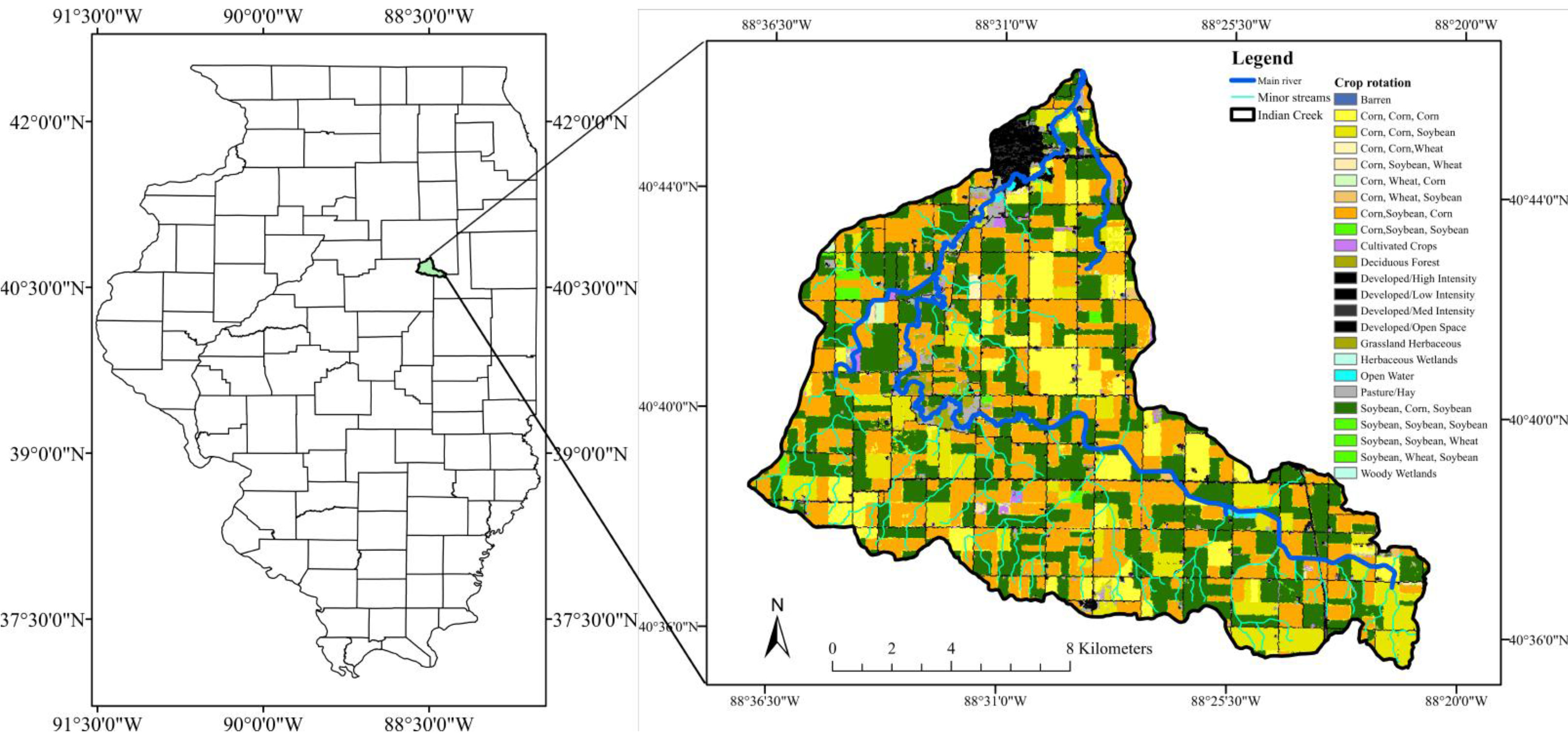
2.1. Study Area

The Indian Creek watershed comprises three 12-digit hydrologic unit code (HUC) subwatersheds (HUCs: 071300020203, 071300020204 and 071300020205) which drain part of the Vermillion River watershed (8-digit HUC; USGS 07130002) that flows into the Illinois River. The watershed covers parts of three Illinois counties of Livingston, McLean, and Ford (Figure 1) and drains approximately 207.4 km² of mostly corn and soybean cropland (>87%) on 104 farms [38]. The major environmental concern in the watershed is excessive nitrate from upland cropland and its impact on public water supply use and aquatic life use (>10 mg·L⁻¹ as monitored by USGS gage 05554300). The mean annual rainfall and mean annual total evapotranspiration are 887 mm and 661 mm, respectively [19]. The three dominant soils in the watershed included (1) Drummer silty clay loam (16.3% of the watershed); (2) Reddick clay loam (9.5%); and (3) Saybrook silt loam (8.8%). Some of the soils in the watershed are susceptible to nitrate leaching. These constituted 6% of the watershed and included the Symerton silt loam and the Varna silty clay loam. Major crop rotations included continuous corn (10.7%), corn-soybean (31.3%), soybean-corn (31.2%), and corn-corn-soybean (11.0%). Crop rotations were generated by overlaying the 2010 to 2012 National Agricultural Statistics Service (NASS) data [39]. The watershed is predominantly under tile drainage due to its low gradient and poorly drained soils; however, there is no readily available data on spatial coverage of the tile-drainage network.

Figure 1. Location of the Indian Creek watershed in the State of Illinois showing the dominant land use and land cover, and three year crop rotations. The watershed drains parts of three Illinois counties of Livingston, Mclean, and Ford into the Vermilion River.

Figure 1. Location of the Indian Creek watershed in the State of Illinois showing the dominant land use and land cover, and three year crop rotations. The watershed drains parts of three Illinois counties of Livingston, Mclean, and Ford into the Vermilion River.

2.2. Data

Two remotely sensed data types, RapidEye and National Agriculture Imagery Program (NAIP) imagery, were used for this study (Table 1). Both images were collected over the Vermillion River watershed. The RapidEye image was collected on 26 August 2011, and the NAIP image consists of image frames collected on 26 August 2011 for our study watershed. The RapidEye satellite imagery consists of blue, green, red, red-edge, and near infrared (NIR) spectral bands at 5 m ground sampling distance at nadir. The RapidEye image was orthorectified by the vendor. The NAIP aerial imagery consists of three visible bands and has 1 m spatial resolution. Both image sets contained less than 10% cloud cover within the scenes.

Table 1. Specification of Remotely Sensed Images.

Type	Spatial Resolution	Spectral Band	Acquisition Date	Radiometric Quantization
National Agriculture Imagery Program (NAIP; aerial)	1 m	Blue, Green, Red	26 August 2011	8 bit
RapidEye (satellite)	5 m	Blue (440–510 nm) Green (520–590 nm) Red (630–685 nm) Red-edge (690–730 nm) NIR (760–850 nm)	26 August 2011	12 bit

Table 1. Specification of Remotely Sensed Images.

Type	Spatial Resolution	Spectral Band	Acquisition Date	Radiometric Quantization
National Agriculture Imagery Program (NAIP; aerial)	1 m	Blue, Green, Red	26 August 2011	8 bit
RapidEye (satellite)	5 m	Blue (440–510 nm) Green (520–590 nm) Red (630–685 nm) Red-edge (690–730 nm) NIR (760–850 nm)	26 August 2011	12 bit

Reference yield data were obtained from corn yield map a 6.5 ha site near the City of Fairbury located in the northern part of the watershed (Fairbury field). The site is under mostly Comfrey loam soils with 0–2% slope. The 2011 corn yields at this site varied between 0.6 and 14 Mg·ha⁻¹ with an average of 9 Mg·ha⁻¹. The georeferenced corn yield map at 15 cm resolution was generated by the John Deere Apex^TM Farm Management Software based on the volumetric grain flow data from the GreenStar^TM yield monitoring system (John Deere Company; Moline, IL, USA) mounted on a combined harvester. Average yields and intra-field variability at this site were consistent with observed watershed values. Observed average corn productivity in the watershed was 9.1 Mg·ha⁻¹ with a 95% confidence interval (95% CI) of 6.2 to 12 Mg·ha⁻¹. These were derived from 2010 to 2013 National Agricultural Statistics Service data (USDA-NASS, 2012) county data, weighted by spatial extent of the three counties in the watershed (Livingston, Ford, and McLean).

2.3. Image Processing and Model Development

The RapidEye image was spatially registered to the NAIP image using 1000+ ground control points to achieve sub-pixel positional accuracy (RMSE < 0.8 pixel). The image-to-image registration was performed using affine transformation with a nearest neighbor resampling method in the ERDAS IMAGINE 2013 AutoSync workstation. The three visible bands of the NAIP image were aggregated to simulate a 1 m resolution panchromatic image. A pansharpening technique was applied to the 5-m RapidEye multispectral image and the 1-m panchromatic image derived from the NAIP image in order to generate a 1-m resolution multispectral image. Using the 1-m pansharpened multispectral image, pixel values of the five spectral bands—blue, green, red, red-edge, and NIR—were extracted from 1500 randomly selected locations within the Fairbury field. A total of 1060 locations that had reference yield values were used as a training dataset for subsequent analyses. Using all possible two-band combinations in the training data, normalized difference band ratios (or normalized difference indices; NDIs) were computed [40] as:

$$NDI=\left(R_a-R_b\right)/\left(R_a+R_b\right)$$

(1)

where R_a and R_b are pixel values of spectral band a and b, respectively. NDIs were selected for this study because the indices such as NDVI are widely known to correlate with crop yield [24,41,42].

To develop a predictive model for crop yield, a multiple linear regression analysis was performed on a total of 15 predictor variables—10 NDIs and five spectral bands of the pansharpened RapidEye image. Predictor variables that were statistically significant (p < 0.01) were included in the model. It should be noted that the spectral bands of remotely sensed imagery are expected to be highly correlated. In our dataset, a principal component analysis suggested that the first two bands explain 99.4% of the variance. Spectral transformations such as a normalized difference band ratio provide information that is less correlated than the original bands via nonlinear transformation of two-band combination. Upon developing a regression model, correlation between predictor variables was examined to account for multicolinearity. When variables are highly correlated (r > 0.90), the one that has higher correlation to yield was kept in the model and the rest of variables were discarded.

The predictive model was applied to the pansharpened RapidEye image, and a predictive yield map was generated. The crop yield map was examined for its reliability based on visual assessment for overall agreement in spatial patterns between the reference and predicted yields. Quantitative reliability in prediction was also examined using F-statistics with p-value, coefficient of determination (R²), and standard error (SE) based on 300 samples selected from random locations. To visualize abundance and spatial configuration of productivity within a field, the predictive yield map was classified into productive and under-productive areas by applying arbitrary percentage of total area of the field (e.g., lowest 10%, 20%, and 30%) for a sample study plot.

2.4. Forecasting of Bioenergy Crop Impact

A calibrated Soil and Water Assessment Tool (SWAT) model for the Indian Creek watershed, IL was used to forecast the impact of growing switchgrass on sub-optimal corn yield areas in the watershed. Watershed corn yields at a subfield scale were estimated using the above developed predictive corn yield model. For details on the calibrated SWAT model refer to Ssegane and Negri [43]. Three assessed scenarios of sub-optimal corn productivity included (1) yields below or equal to 3.1 Mg·ha⁻¹; (2) yields below or equal to 4.7 Mg·ha⁻¹; and (3) yields below or equal to 6.3 Mg·ha⁻¹. The three thresholds are equivalent to approximately 30%, 50%, and 70% of observed average corn productivity in the watershed of 9.1 Mg·ha⁻¹. Next, SWAT was modified to model an alternative landscape where switchgrass replaced current land use and land cover at a subfield level on areas meeting each of the three scenarios. The forecast evaluated the impact of conversion to switchgrass on annual corn and soybean yields, NO₃-N and sediment exports, and water yield. Statistical assessments of pairwise differences in nutrient exports under different scenarios were achieved using a non-parametric Mann-Whitney test [44].

3. Results

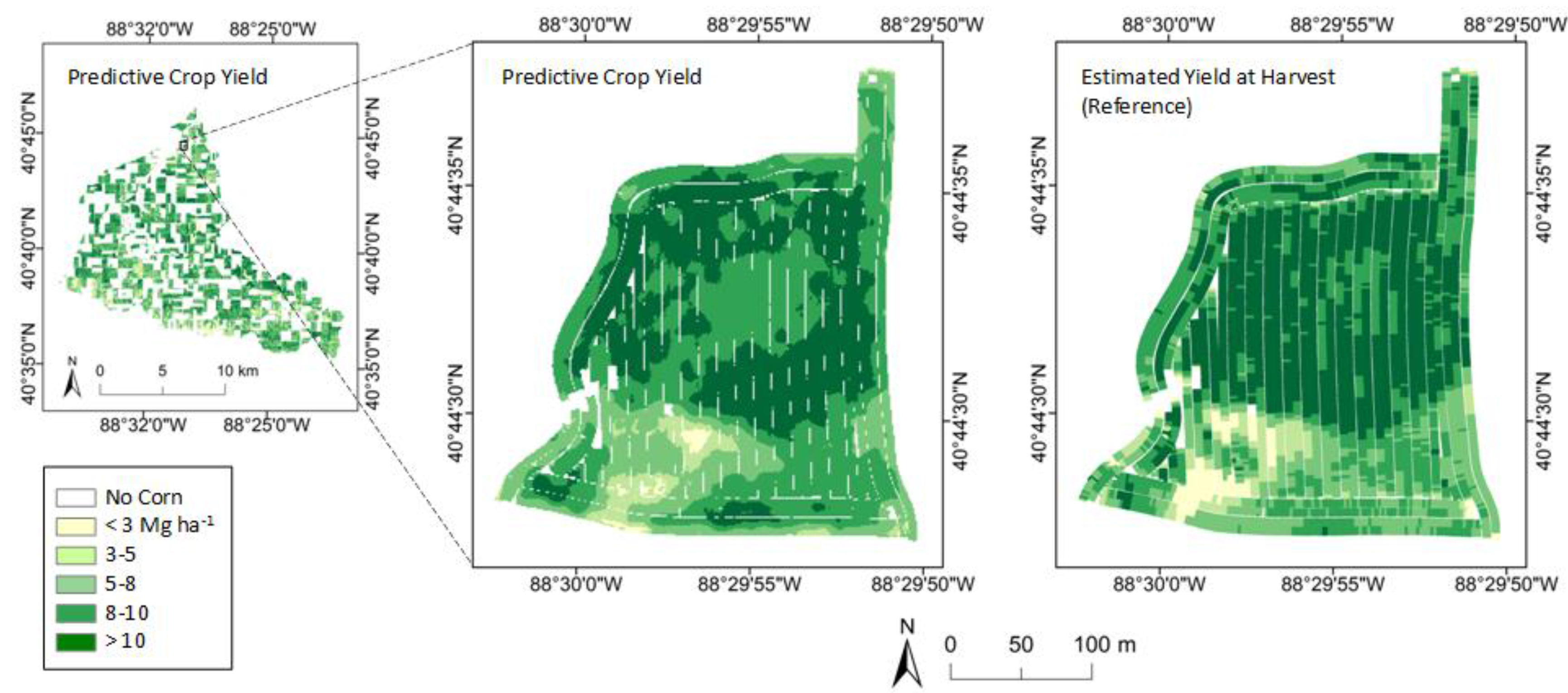
3.1. Regression Model for Predictive Yield

The regression analysis of 10 NDIs and five spectral bands indicated that four variables—red and NIR bands, a NDI using red-NIR combination (known as NDVI; [34]), and a NDI using red-edge-NIR combination (known as red-edge normalized difference vegetation index or RENDVI; [45])—were significant predictors for crop yield (p < 0.01). Among the four variables, correlation between NDVI and RENDVI were 0.94; thus, RENDVI that had higher correlation with yield (R² = 0.733) was selected for the model instead of NDVI (R² = 0.711). The final multiple linear regression model for predicting crop yield was as follows:

$$\text{Yield} \left(\text{Mg}·{\text{ha}}^{-1}\right)=0.0009107\times B3+0.0001729\times B5+4.531\times \text{RENDVI}-1.301$$

(2)

where B3 and B5 are red and NIR spectral bands, respectively. The model showed a large F-value (F = 418) with statistical significance (p < 0.001) and the coefficient of determination (R² = 0.543) with standard error (SE) of 1.635. The regression model was applied to the pansharpened RapidEye image to map predictive crop yield.

The predictive yield map of the study plot derived from the model was shown in Figure 2. The predicted yield showed striking similarity to the reference yield estimated at harvest. High yield appeared to be concentrated in the central portion of the field with a couple of small isolated distributions in the southern part of the field. Considerably lower yield was observed in the southern portion section of the field particularly near the mid-section. Overall the model is statistically significant (p < 0.001) with a large F-value (F = 328). Correlation (R²) between the predicted and reference yield was 0.524, and estimated error (SE) in prediction was 1.61.

Figure 2. Predicted corn yield maps generated based on the regression model of the watershed (left) and the study field (center); and reference yield map at harvest (right).

Figure 2. Predicted corn yield maps generated based on the regression model of the watershed (left) and the study field (center); and reference yield map at harvest (right).

The predictive yield map was classified into two areas—productive and under-productive. Sample classification of the study field shown in Figure 3 were based on the three areal proportions—10%, 20% and 30% of total area. Areas of low productivity are primarily concentrated in the southern portion of the field in a spatially contiguous manner across the three classification maps. The 10% of total area exhibiting low productivity coincides with part of the eroded Symerton silt loam soil series with slope gradients of 5%–10%. With the 30% threshold, under-productive areas coincide with most of the eroded Symerton silt loam soil series with slopes of 5%–10% and parts of the same soil series with slopes of 2%–5%. These soils have less organic matter and are more susceptible to NO₃-N leaching. The high yield areas are on the Comfrey loam soils with slopes of 0%–2% and are not susceptible to NO₃-N leaching. In addition to the distribution, the maps also indicate size and connectivity of under-productive areas within the field.

Figure 3. Examples of stratification of under-productive land by percent area in Fairbury Field.

Figure 3. Examples of stratification of under-productive land by percent area in Fairbury Field.

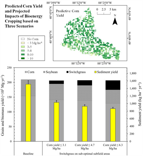
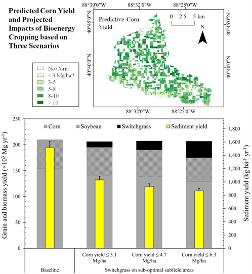
3.2. Simulated Grain and Switchgrass Yields

The total area in the watershed meeting the three corn yield thresholds of 3.1 Mg·ha⁻¹, 4.7 Mg·ha⁻¹, and 6.3 Mg·ha⁻¹, were 646 ha (3.2% of the watershed), 1487 ha (7.4%), and 2892 ha (14.3%), respectively. When areas whose corn yield productivity were less or equal to 3.1 Mg·ha⁻¹ were converted to switchgrass (scenario 1), annual total grain yields were projected to reduce by 6.9% (Figure 4). However, this land use conversion projected 10,664 metric tons of switchgrass biomass. Conversion of areas at or below corn productivity thresholds of 4.7 Mg·ha⁻¹ and 6.3 Mg·ha⁻¹ were projected to decrease annual total grain yields by 9.4% and 16.6%, respectively. For example, under the second scenario, 19,642 metric tons of grain (Corn: 15,876 and Soybean: 3766) were lost from the baseline 209,810 metric tons. Projected switchgrass biomass was 16,797 metric tons. Yield projections under the third scenario (6.3 Mg·ha⁻¹ threshold) predicted a reduction of 34,747 metric tons (Corn: 24,919 and Soybean: 9828) from baseline annual total grain yields. Projected switchgrass biomass yield under the third scenario was 31,522 metric tons. The figure also shows substantial decrease in sediment yield under all three scenarios (25%–39% reduction).

3.3. Forecasted Impact on Water Quality and Quantity

Conversions of watershed areas whose corn productivity was less or equal to 3.1 Mg·ha⁻¹, 4.7 Mg·ha⁻¹, and 6.3 Mg·ha⁻¹, on average were projected to reduce tile NO₃-N leachate by 15.9%, 18.4% and 25.9%, respectively (Figure 5a). For sediment, the corresponding respective reductions were 25%, 35.5% and 39% (Figure 5b), while, for water yield, the reductions were 0.9%, 1.1% and 2.5% (Figure 5c). Figure 5 shows that the reductions in tile NO₃-N are not significantly different (p > 0.05) for Cases 1 and 2 (3.2% and 7.4% of the watershed). However, the corresponding reductions in sediment export are. This was attributed to a relatively higher reduction in annual surface runoff (92.8 mm vs. 90.7 mm) compared to the increase in annual tile-flow (118.4 mm vs. 120.1 mm). Average reductions in annual NO₃-N export and sediment yield were projected to be over 10% and therefore considered hydrologically significant for all three land cover change scenarios because these changes are higher than typical probable errors associated with data measurement and sample collection [46]. Projected reductions in water yield under all three scenarios were below 10% and therefore not hydrologically significant.

Figure 4. Grain and biomass yields (corn, soybean, and switchgrass biomass) for the baseline (current land use and land cover) and three suboptimal corn yield productivity scenarios of less or equal to 3.1 Mg·ha⁻¹, 4.7 Mg·ha⁻¹, and 6.3 Mg·ha⁻¹. The error bars are standard errors.

Figure 4. Grain and biomass yields (corn, soybean, and switchgrass biomass) for the baseline (current land use and land cover) and three suboptimal corn yield productivity scenarios of less or equal to 3.1 Mg·ha⁻¹, 4.7 Mg·ha⁻¹, and 6.3 Mg·ha⁻¹. The error bars are standard errors.

Figure 5. Relative reductions in: (a) NO₃-N export; (b) sediment yield; and (c) water yield under different areal extents of land use change derived from applying three corn productivity thresholds of 3.1 Mg·ha⁻¹ (Case 1), 4.7 Mg·ha⁻¹ (Case 2), and 6.3 Mg·ha⁻¹ (Case 3). The corresponding areal coverages are 3.2% of the watershed, 7.4%, and 14.3%, respectively. The relative reductions are comparisons between current land use (baseline condition) and conversion of areas below the above yield thresholds to switchgrass.

Figure 5. Relative reductions in: (a) NO₃-N export; (b) sediment yield; and (c) water yield under different areal extents of land use change derived from applying three corn productivity thresholds of 3.1 Mg·ha⁻¹ (Case 1), 4.7 Mg·ha⁻¹ (Case 2), and 6.3 Mg·ha⁻¹ (Case 3). The corresponding areal coverages are 3.2% of the watershed, 7.4%, and 14.3%, respectively. The relative reductions are comparisons between current land use (baseline condition) and conversion of areas below the above yield thresholds to switchgrass.

4. Discussion

The multiple regression model developed using a high-resolution multispectral image showed modest performance for predicting crop yield, yet the predictive yield map showed considerable resemblance with the reference yield map. The coefficient of determination (R² = 0.52) and SE = 0.16 suggests that approximately 52% of variability in yield is explained by the three terms in the model (i.e., reflectance values of the red and NIR bands and RENDVI), and a typical deviation of predicated yield from the reference yield is 1.61 Mg·ha⁻¹. Timing of image collection was considered to have substantial impact on the correlation between SVIs and crop yield. Based on the analysis of SVIs and crop phenology metrics derived from the 250-m MODIS products, Bolton and Friedl [24] determined that approximately 65–75 days and 80 days after greenup were optimal timing of image collection for predicting yield for corn and soybean, respectively. Typical greenup of corn in our study watershed is in late May, and the image data collected on 26 August, was approximately a few weeks later than the optimal date. While high resolution satellite imagery has promise for providing sub-field level information, it is challenging to acquire imagery having desired spectral bands at the optimal time of the year with good sky condition. The use of an aerial platform would permit control over image collection dates and sky conditions, but mission planning and standardization of data over time would be challenging and costly.

The difference between predicted and reference yield most likely stemmed from the indirect nature of yield prediction using remote sensing. Spectral reflectance signatures of crops are primarily influenced by plant’s physical properties (e.g., chlorophyll content, mesophyll structure, canopy architecture, and biomass). We predicted yield indirectly by determining a relationship between the spectral reflectance signatures and crop yield [47,48]. Positional misalignment and the difference in spatial resolution between the image and the reference yield data were also sources of uncertainty. The reference yield data was reprojected to improve spatial alignment with the RapidEye image. Some discrepancy could have been introduced during the transformation of the reference data, which could have influenced the predictive power of the model. The reference yield data also exhibited a blocky pattern that was created by multiple spatially contiguous pixels having a common yield value although the yield was recorded at 15 cm resolution. The block size varies across the field ranging from approximately 4 m² to 12 m². This pattern appeared as multiple index values falling in a single yield value in Figure 2. The use of appropriate spatial scales in conjunction with careful spatial registration between field measurement and input image is expected to improve accuracy in predictive yield.

Normalized difference indices based on ratios of two multispectral bands were tested for their effectiveness for predicting crop yield in this study. More exhaustive analysis of spectral indices (such as simple ratios and differences) and angle indices derived from the angle formed by three spectral bands in a multispectral signature plot [49], in conjunction with partial least square regression [50] or random forest regression [40] may improve accuracy of yield estimates. Recent examples for yield estimates using remote sensing are provided in Rembold et al. [48].

Theoretically, computing predictive yields across a small watershed using remote sensing is feasible. Because of heterogeneity of soil conditions within the watershed, however, further investigation is warranted to determine how well we can predict yields using a single-date image. Additional information such as crop types, planting date, and fertilizer application for each field [51,52] in conjunction with careful selection of the image collection timing would improve the accuracy of yield prediction. If the use of a single image is found insufficient, it is important to learn about the minimum number of images [24,53] needed for reliable yield prediction in order to keep manageable operational cost.

Spatial comprehensive information of predictive yield, particularly with sub-field yield, provides valuable information for farmers to plan their land use at a very fine spatial scale that meets their objectives and for land and watershed planners to design landscapes to deliver specific conservation targets. The demonstration presented in this study is one example based on the proportional area characterized by low predictive yield. Farmers could use the information to determine a certain proportion of the field for alternative or experimental crops without sacrificing yield. Spatial representation of predictive yield also provides valuable information such as size, proximity, spatial arrangement, and connectivity of under-productive areas (Figure 3), which simple statistics or numerical information does not provide. The predictive yield maps at a resolution that can resolve variability of yields and its spatial patterns would be valuable for farmers in planning their sub-field scale land use in order to achieve their production goals while mitigating impacts on ecosystem services and environment. The information can be used to examine accessibility of areas by large equipment, efficiency of management for multiple areas, and potential impacts on primary crop adjacent to areas that experience alternative treatment/management. There are multiple ways to define under-productive areas such as based on predictive yield or multi-year yield record. Criteria for under-productive areas should be determined based on the objectives.

For this study, we do not make the assumption that the financial loss due to the acreage put out of grain production is directly compensated by the switchgrass yield. Because current market valuation frameworks do not reflect the full benefits of the ecosystem services associated with such land cover conversions. However, current and future work on valuation frameworks of the accrued ecosystem services may reflect the true cost and benefit ratio of these integrated systems and thus make them more acceptable to farmers.

5. Conclusions

Biofuels derived from renewable biological materials are important alternatives for meeting our future energy needs. A sustainable integration of new bioenergy crops within existing cropping systems requires a landscape design that identifies sub-field scale details to correctly allocate land based on its fertility and productivity to the best matching crops. This design allows the bioenergy crops to perform important ecosystem services in balance with the production of bioenergy feedstock and commodity crops. To facilitate sustainable bioenergy crop production, this study demonstrated the utility of single date, high resolution remote sensing and hydrologic modeling for determining under-productive areas within a plot and examining impacts of using those areas to grow bioenergy crops. The findings are summarized as follows:

• The regression model using the red and near infrared spectral bands and the red-edge normalized difference vegetation index showed the best performance for predicting crop yield (R² = 0.524; p < 0.001; standard error = 1.61) of all variables tested.
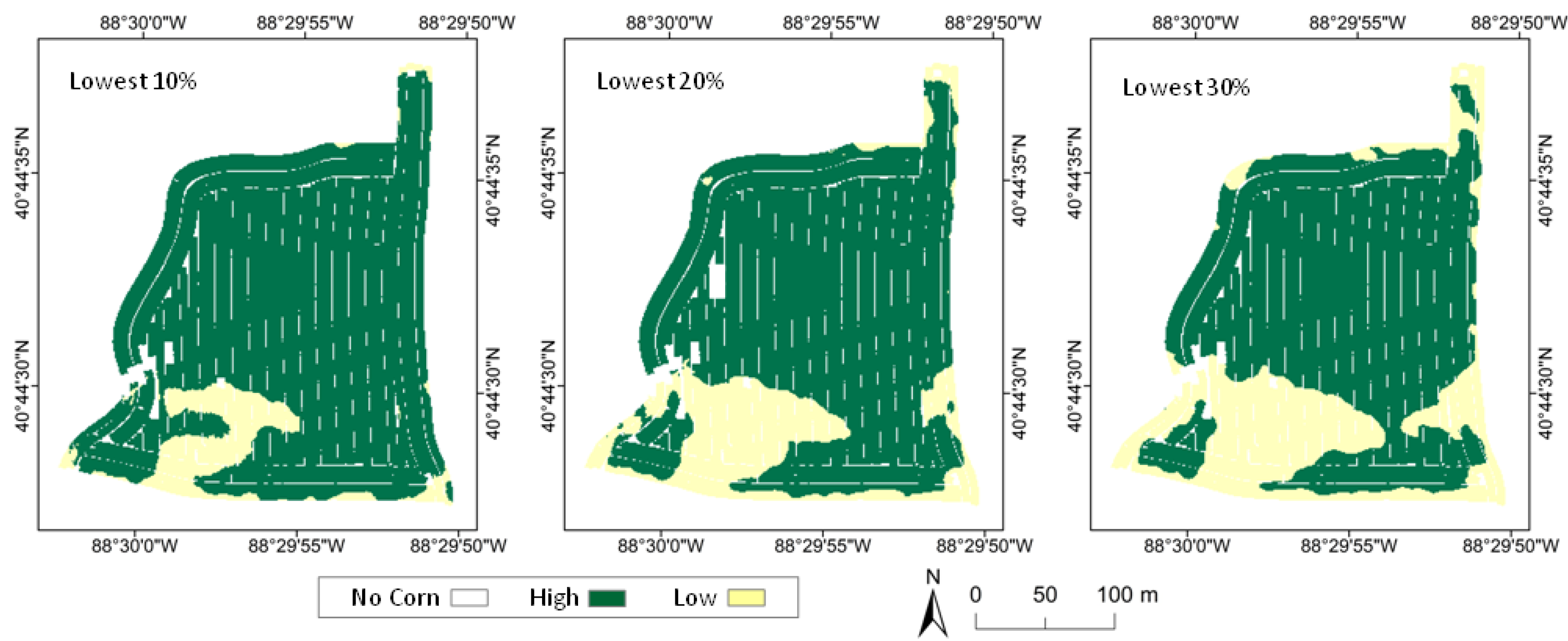
• The predictive yield map showed that under-productivity areas largely coincide with the eroded Symerton silt loam soil series with slope gradient of 5%–10%.
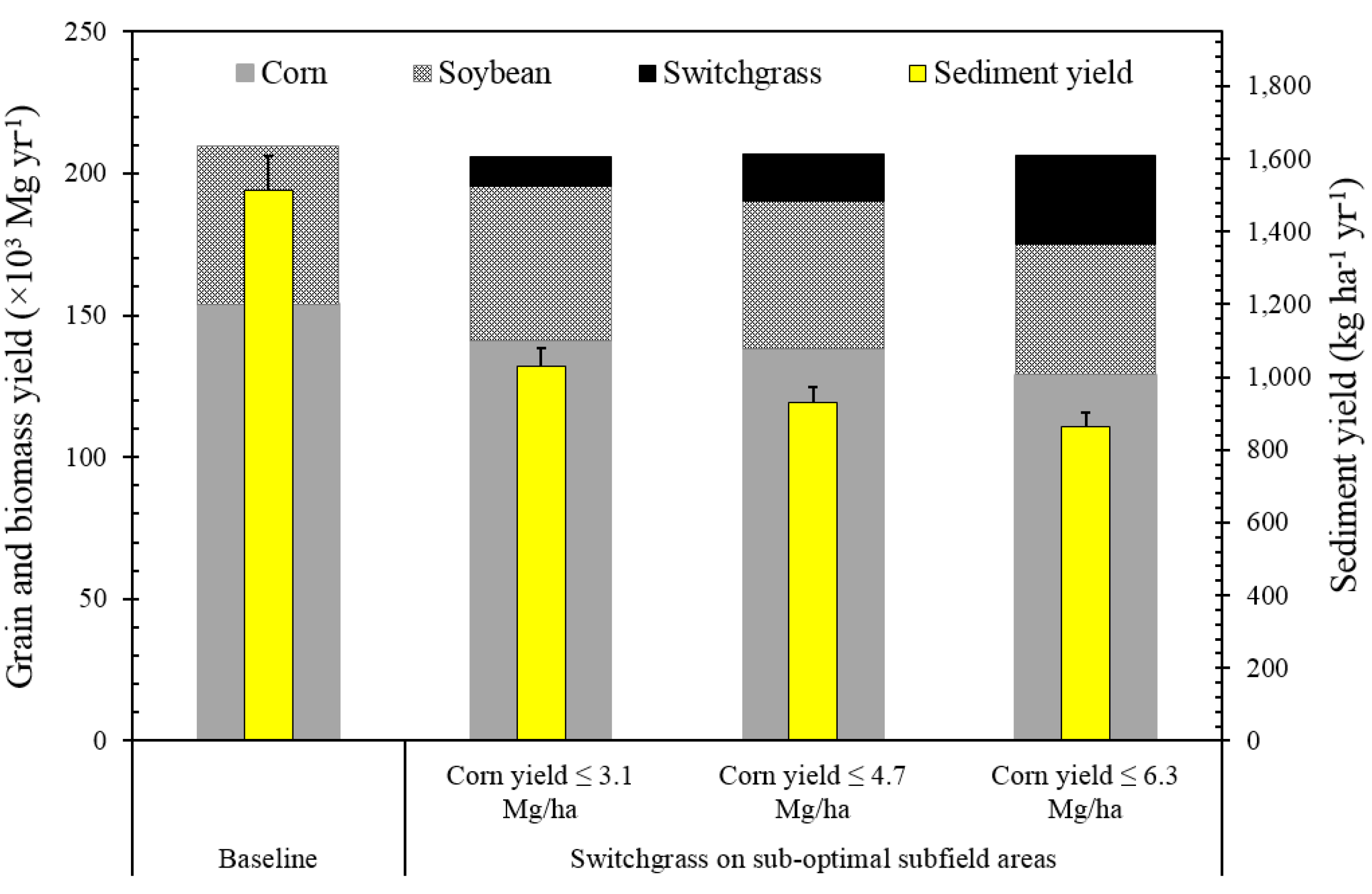
• When testing three scenarios of corn-to-switchgrass conversion for areas with predicted corn yield less than or equal to 3.1, 4.7 and 6.3 Mg·ha⁻¹, total grain yield was projected to decrease from baseline by 6.9%, 9.4% and 16.6%, respectively, and the corresponding switchgrass biomass production was projected to be 10,664, 16,797, and 31,522 metric tons, respectively.
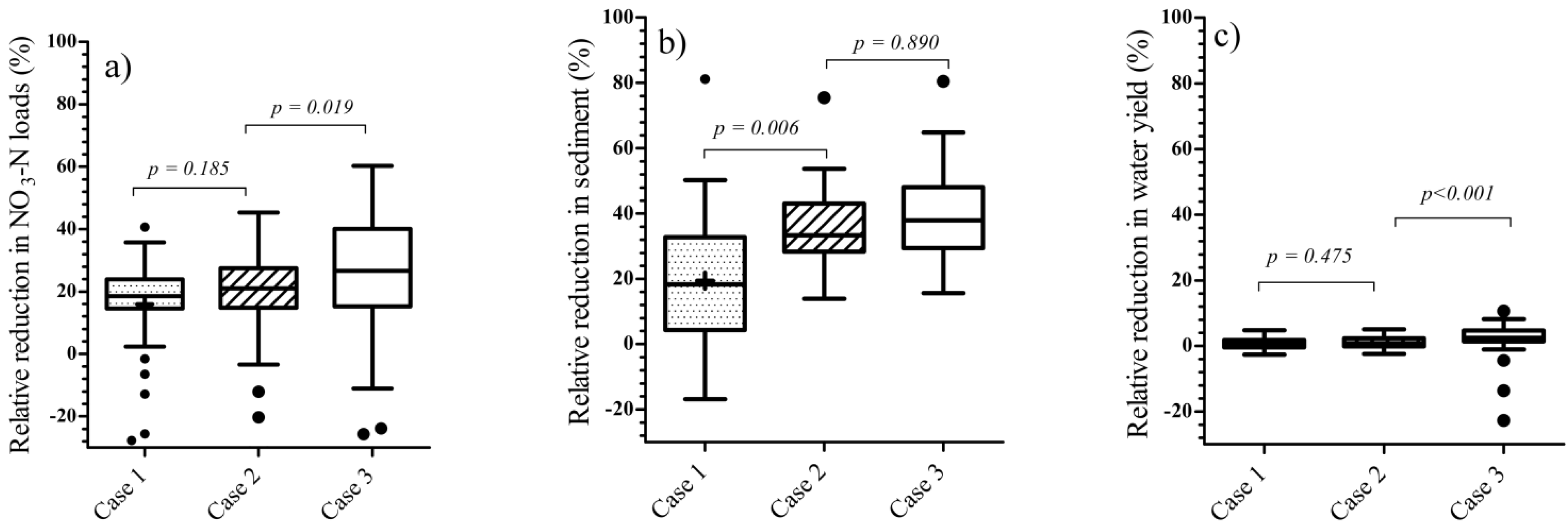
• Between scenarios 1 and 2, the reduction in tile NO₃-N transport was not significantly different (15.9% vs. 18.4% reduction, respectively) while the reduction in sediment yield was (25% vs. 35.5%, respectively).

While there is more work to be conducted, this study is a first attempt to demonstrate the promise of remote sensing technology to deliver actionable data for landscape design, by resolving at an unprecedented resolution, issues related to land marginality, spatially constrained productivity and optimal land allocation to meet specific functional objectives at the decision-making scale. It has been shown that land use decisions regarding privately owned land are made at the field, farm, and watershed scales. Such a methodology would be an invaluable tool in allowing this decision making to prioritize crop selection, specific yield and conservation objectives that are the basis for sustainable agricultural practices. In addition to determining the robustness of the model using multiple plots across the watershed, future studies should include determining the limitation of a single date, high resolution multispectral image for accurately predicting crop yield at a subplot scale, and testing exhaustive spectral indices and other techniques (e.g., partial least square regression and random forest regression) to improve prediction accuracy.

References

1. Baker, J.M.; Fassbinder, J.; Lamb, J.A. The impact of corn stover removal on N2O emission and soil respiration: An investigation with automated chambers. Bioenergy Res. 2014, 7, 503–508. [Google Scholar]
2. Campbell, E.E.; Johnson, J.M.F.; Jin, V.L.; Lehman, R.M.; Osborne, S.L.; Varvel, G.E.; Paustian, K. Assessing the soil carbon, biomass production, and nitrous oxide emission impact of corn stover management for bioenergy feedstock production using DAYCENT. Bioenergy Res. 2014, 7, 491–502. [Google Scholar] [CrossRef]
3. Cibin, R.; Chaubey, I.; Engel, B. Simulated watershed scale impacts of corn stover removal for biofuel on hydrology and water quality. Hydrol. Process. 2012, 26, 1629–1641. [Google Scholar] [CrossRef]
4. Thomas, M.A.; Engel, B.A.; Chaubey, I. Multiple corn stover removal rates for cellulosic biofuels and long-term water quality impacts. J. Soil Water Conserv. 2011, 66, 431–444. [Google Scholar] [CrossRef]
5. Blanco-Canqui, H.; Lal, R. Corn stover removal for expanded uses reduces soil fertility and structural stability. Soil Sci. Soc. Am. J. 2009, 73, 418–426. [Google Scholar] [CrossRef]
6. Thompson, J.L.; Tyner, W.E. Corn stover for bioenergy production: Cost estimates and farmer supply response. Biomass Bioenergy 2014, 62, 166–173. [Google Scholar] [CrossRef]
7. Hong, B.G.; Swaney, D.P.; Howarth, R.W. Estimating net anthropogenic nitrogen inputs to us watersheds: Comparison of methodologies. Environ. Sci. Technol. 2013, 47, 5199–5207. [Google Scholar] [CrossRef] [PubMed]
8. McIsaac, G.F.; David, M.B.; Gertner, G.Z.; Goolsby, D.A. Relating net nitrogen input in the Mississippi river basin to nitrate flux in the lower Mississippi river: A comparison of approaches. J. Environ. Qual. 2002, 31, 1610–1622. [Google Scholar] [CrossRef] [PubMed]
9. Goolsby, D.A.; Battaglin, W.A.; Aulenbach, B.T.; Hooper, R.P. Nitrogen input to the gulf of Mexico. J. Environ. Qual. 2001, 30, 329–336. [Google Scholar] [CrossRef] [PubMed]
10. Keeler, B.L.; Krohn, B.J.; Nickerson, T.A.; Hill, J.D. US federal agency models offer different visions for achieving renewable fuel standard (RFS2) biofuel volumes. Environ. Sci. Technol. 2013, 47, 10095–10101. [Google Scholar] [CrossRef] [PubMed]
11. Gopalakrishnan, G.; Cristina Negri, M.; Snyder, S.W. A novel framework to classify marginal land for sustainable biomass feedstock production. J. Environ. Qual. 2011, 40, 1593–1600. [Google Scholar] [CrossRef] [PubMed]
12. Milbrandt, A.R.; Heimiller, D.M.; Perry, A.D.; Field, C.B. Renewable energy potential on marginal lands in the United States. Renew. Sustain. Energy Rev. 2014, 29, 473–481. [Google Scholar] [CrossRef]
13. Varvel, G.E.; Vogel, K.P.; Mitchell, R.B.; Follett, R.; Kimble, J. Comparison of corn and switchgrass on marginal soils for bioenergy. Biomass Bioenergy 2008, 32, 18–21. [Google Scholar] [CrossRef]
14. Zhuang, D.; Jiang, D.; Liu, L.; Huang, Y. Assessment of bioenergy potential on marginal land in China. Renew. Sustain. Energy Rev. 2011, 15, 1050–1056. [Google Scholar] [CrossRef]
15. Dangerfield, C., Jr.; Harwell, R. An analysis of a silvopastoral system for the marginal land in the southeast United States. Agrofor. Syst. 1990, 10, 187–197. [Google Scholar] [CrossRef]
16. Gelfand, I.; Sahajpal, R.; Zhang, X.S.; Izaurralde, R.C.; Gross, K.L.; Robertson, G.P. Sustainable bioenergy production from marginal lands in the US Midwest. Nature 2013, 493, 514–517. [Google Scholar] [CrossRef] [PubMed]
17. Harvolk, S.; Kornatz, P.; Otte, A.; Simmering, D. Using existing landscape data to assess the ecological potential of Miscanthus cultivation in a marginal landscape. GCB Bioenergy 2014, 6, 227–241. [Google Scholar] [CrossRef]
18. Zumkehr, A.; Campbell, J. Historical US cropland areas and the potential for bioenergy production on abandoned croplands. Environ. Sci. Technol. 2013, 47, 3840–3847. [Google Scholar] [CrossRef] [PubMed]
19. Ssegane, H.; Negri, M.C.; Quinn, J.; Urgun-Demirtas, M. Multifunctional landscapes: Site characterization and field-scale design to incorporate biomass production into an agricultural system. Biomass Bioenergy 2015, 80, 179–190. [Google Scholar] [CrossRef]
20. Basso, B.; Cammarano, D.; Carfagna, E. Review of Crop Yield Forecasting Methods and Early Warning Systems. 2014, Volume 2014. Available online: http://www.fao.org/fileadmin/templates/ess/documents/meetings_and_workshops/GS_SAC_2013/Improving_methods_for_crops_estimates/Crop_Yield_Forecasting_Methods_and_Early_Warning_Systems_Lit_review.pdf (accessed on 28 July 2015).
21. Campbell, J.B. Introduction to Remote Sensing; CRC Press: Boca Raton, FL, USA, 2002. [Google Scholar]
22. Slaton, M.R.; Hunt, E.R.; Smith, W.K. Estimating near-infrared leaf reflectance from leaf structural characteristics. Am. J. Bot. 2001, 88, 278–284. [Google Scholar] [CrossRef] [PubMed]
23. Doraiswamy, P.C.; Hatfield, J.L.; Jackson, T.J.; Akhmedov, B.; Prueger, J.; Stern, A. Crop condition and yield simulations using Landsat and MODIS. Remote Sens. Environ. 2004, 92, 548–559. [Google Scholar] [CrossRef]
24. Bolton, D.K.; Friedl, M.A. Forecasting crop yield using remotely sensed vegetation indices and crop phenology metrics. Agric. For. Meteorol. 2013, 173, 74–84. [Google Scholar] [CrossRef]
25. Huang, Y.; Liu, X.; Shen, Y.; Jin, J. Assessment of agricultural drought indicators impact on soybean crop yield: A case study in Iowa, USA. In Proceedings of the Third International Conference on Agro-Geoinformatics (Agro-Geoinformatics 2014), Beijing, China, 11–14 August 2014; pp. 1–6.
26. Sibley, A.M.; Grassini, P.; Thomas, N.E.; Cassman, K.G.; Lobell, D.B. Testing remote sensing approaches for assessing yield variability among maize fields. Agron. J. 2014, 106, 24–32. [Google Scholar] [CrossRef]
27. Li, A.N.; Liang, S.L.; Wang, A.S.; Qin, J. Estimating crop yield from multi-temporal satellite data using multivariate regression and neural network techniques. Photogramm. Eng. Remote Sens. 2007, 73, 1149–1157. [Google Scholar] [CrossRef]
28. Topaloglou, C.; Monachou, S.; Strati, S.; Alexandridis, T.; Stavridou, D.; Silleos, N.; Misopolinos, N.; Nunes, A.; Araujo, A. Modeling LAI based on land cover map and NDVI using SPOT and Landsat data in two Mediterranean sites: Preliminary results. Proc. SPIE 2013, 8795. [Google Scholar] [CrossRef]
29. Araujo, G.K.D.; Rocha, J.V.; Lamparelli, R.A.C.; Rocha, A.M. Mapping of summer crops in the state of Parana, Brazil, through the 10-day SPOT vegetation NDVI composites. Eng. Agric. 2011, 31, 760–770. [Google Scholar] [CrossRef]
30. Enclona, E.; Thenkabail, P.; Celis, D.; Diekmann, J. Within-field wheat yield prediction from IKONOS data: A new matrix approach. Int. J. Remote Sens. 2004, 25, 377–388. [Google Scholar] [CrossRef]
31. Alganci, U.; Ozdogan, M.; Sertel, E.; Ormeci, C. Estimating maize and cotton yield in southeastern Turkey with integrated use of satellite images, meteorological data and digital photographs. Field Crops Res. 2014, 157, 8–19. [Google Scholar] [CrossRef]
32. Konecny, G. Geoinformation: Remote Sensing, Photogrammetry and Geographic Information Systems; CRC Press: Boca Raton, FL, USA, 2014. [Google Scholar]
33. Shanahan, J.F.; Schepers, J.S.; Francis, D.D.; Varvel, G.E.; Wilhelm, W.W.; Tringe, J.M.; Schlemmer, M.R.; Major, D.J. Use of remote-sensing imagery to estimate corn grain yield. Agron. J. 2001, 93, 583–589. [Google Scholar] [CrossRef]
34. Tucker, C.J. Red and photographic infrared linear combinations for monitoring vegetation. Remote Sens. Environ. 1979, 8, 127–150. [Google Scholar] [CrossRef]
35. Baret, F.; Guyot, G.; Major, D. TSAVI: A vegetation index which minimizes soil brightness effects on LAI and APAR estimation. In Proceedings of the 12th Canadian Symposium on Remote Sensing, Geoscience and Remote Sensing Symposium, IGARSS’89, Vancouver, BC, Canada, 10–14 July 1989; pp. 1355–1358.
36. Gitelson, A.A.; Kaufman, Y.J.; Merzlyak, M.N. Use of a green channel in remote sensing of global vegetation from EOS-MODIS. Remote Sens. Environ. 1996, 58, 289–298. [Google Scholar] [CrossRef]
37. Cicek, H.; Sunohara, M.; Wilkes, G.; McNairn, H.; Pick, F.; Topp, E.; Lapen, D. Using vegetation indices from satellite remote sensing to assess corn and soybean response to controlled tile drainage. Agric. Water Manag. 2010, 98, 261–270. [Google Scholar] [CrossRef]
38. Maier, M. Protecting water with on-farm conservation: The Indian creek watershed project. In Proceeding of the National Workshop on Large Landscape Conservation, Washington, DC, USA, 23–24 October 2014.
39. USDA-NASS. Cropscape-Cropland Data Layer. US Department of Agriculture, National Agricultural Statistics Service: Washington, 2012. Available online: http://nassgeodata.gmu.edu/CropScape (accessed on 20 August 2013). [Google Scholar]
40. Mutanga, O.; Adam, E.; Cho, M.A. High density biomass estimation for wetland vegetation using worldview-2 imagery and random forest regression algorithm. Int. J. Appl. Earth Obs. 2012, 18, 399–406. [Google Scholar] [CrossRef]
41. Thenkabail, P.S.; Smith, R.B.; de Pauw, E. Hyperspectral vegetation indices and their relationships with agricultural crop characteristics. Remote Sens. Environ. 2000, 71, 158–182. [Google Scholar] [CrossRef]
42. Wall, L.; Larocque, D.; Léger, P.M. The early explanatory power of NDVI in crop yield modelling. Int. J. Remote Sens. 2008, 29, 2211–2225. [Google Scholar] [CrossRef]
43. Ssegane, H.; Negri, M.C. Designing a sustainable integrated landscape for commodity and bioenergy crops in a tile-drained agricultural watershed. GCB Bioenergy 2015. under review. [Google Scholar]
44. Yue, S.; Wang, C. Power of the mann-whitney test for detecting a shift in median or mean of hydro-meteorological data. Stoch. Environ. Res. Risk Assess. 2002, 16, 307–323. [Google Scholar] [CrossRef]
45. Gitelson, A.; Merzlyak, M.N. Spectral reflectance changes associated with autumn senescence of Aesculus hippocastanum L. and Acer platanoides L. Leaves. Spectral features and relation to chlorophyll estimation. J. Plant Physiol. 1994, 143, 286–292. [Google Scholar] [CrossRef]
46. Harmel, R.; Cooper, R.; Slade, R.; Haney, R.; Arnold, J. Cumulative uncertainty in measured streamflow and water quality data for small watersheds. Trans. Am. Soc. Agric. Eng. 2006, 49. [Google Scholar] [CrossRef]
47. Delécolle, R.; Maas, S.; Guérif, M.; Baret, F. Remote sensing and crop production models: Present trends. ISPRS J. Photogramm. Remote Sens. 1992, 47, 145–161. [Google Scholar] [CrossRef]
48. Rembold, F.; Atzberger, C.; Savin, I.; Rojas, O. Using low resolution satellite imagery for yield prediction and yield anomaly detection. Remote Sens. 2013, 5, 1704–1733. [Google Scholar] [CrossRef] [Green Version]
49. Richter, K.; Atzberger, C.; Vuolo, F.; Urso, G.D. Evaluation of sentinel-2 spectral sampling for radiative transfer model based LAI estimation of wheat, sugar beet, and maize. IEEE J. Sel. Top. Appl. Earth Obs. Remote Sens. 2011, 4, 458–464. [Google Scholar] [CrossRef]
50. Atzberger, C.; Guérif, M.; Baret, F.; Werner, W. Comparative analysis of three chemometric techniques for the spectroradiometric assessment of canopy chlorophyll content in winter wheat. Comput. Electron. Agric. 2010, 73, 165–173. [Google Scholar] [CrossRef]
51. Munkholm, L.J.; Heck, R.J.; Deen, B. Long-term rotation and tillage effects on soil structure and crop yield. Soil Tillage Res. 2013, 127, 85–91. [Google Scholar] [CrossRef]
52. Reddy, B.; Reddy, P.S.; Bidinger, F.; Blümmel, M. Crop management factors influencing yield and quality of crop residues. Field Crops Res. 2003, 84, 57–77. [Google Scholar] [CrossRef] [Green Version]
53. Sakamoto, T.; Gitelson, A.A.; Arkebauer, T.J. MODIS-based corn grain yield estimation model incorporating crop phenology information. Remote Sens. Environ. 2013, 131, 215–231. [Google Scholar] [CrossRef]