Coupled Ground- and Space-Based Assessment of Regional Inundation Dynamics to Assess Impact of Local and Upstream Changes on Evaporation in Tropical Wetlands

Schwerdtfeger, Julia; Da Silveira, Sérgio Wagner Gripp; Zeilhofer, Peter; Weiler, Markus

doi:10.3390/rs70809769

Open AccessArticle

Coupled Ground- and Space-Based Assessment of Regional Inundation Dynamics to Assess Impact of Local and Upstream Changes on Evaporation in Tropical Wetlands

by

Julia Schwerdtfeger

^1,*,

Sérgio Wagner Gripp Da Silveira

²,

Peter Zeilhofer

² and

Markus Weiler

¹

Chair of Hydrology, Faculty of Environment and Natural Resources, University of Freiburg, Fahnenbergplatz, 79098 Freiburg, Germany

²

Pos-Graduação em Física Ambiental, Instituto de Física, Universidade Federal de Mato Grosso (UFMT), Avenida Fernando Correa da Costa n° 2367, Boa Esperança, 78060900 Cuiabá, Brazil

^*

Author to whom correspondence should be addressed.

Remote Sens. 2015, 7(8), 9769-9795; https://doi.org/10.3390/rs70809769

Submission received: 17 March 2015 / Revised: 27 July 2015 / Accepted: 28 July 2015 / Published: 31 July 2015

Download

Browse Figures

Versions Notes

Abstract

:

Modifications of human land use and climate change are known to be a threat for the health and proper functioning of tropical wetlands. They interfere with the seasonal flood pulse, which is seen as the most important driver for biodiversity and directly controls evaporation. In order to investigate the impact of local and upstream changes on wetlands, a regional assessment of evaporation is crucial but challenging in such often remote and poorly gauged ecosystems. Evaporation is the major water balance component of these wetlands and links the flood pulse with the ecosystem. It can therefore be seen as a proxy for their functioning. In the last decades, information from space became an important data source to assess remote wetland areas. Here, we developed a new approach to quantify regional evaporation driven by inundation dynamics as its dominant control. We used three water and vegetation indices (mNDWI (modified Normalized Difference Water Index), NDVI (Normalized Difference Vegetation Index), and EVI (Enhanced Vegetation Index)) from MODIS (Moderate Resolution Imaging Spectroradiometer) surface reflectance products to assess regional inundation dynamics between the dry and wet seasons. Two years of continual in situ water level measurements at different locations in our study area, the Pantanal wetland of South America, provided the reference to evaluate our method. With process-based modeling that used the inundation dynamics to determine the water available for evaporation, we were able to estimate actual evaporation (AET) on a regional scale. Relating AET to changes in discharge due to upstream flow modifications and on local precipitation over the last 13 years, we found that the Pantanal is more vulnerable to alternated inundation dynamics than to changes in local precipitation. We concluded that coupling ground- and space-based information in this remote wetland area is a valuable first step to investigate the status of the Pantanal ecosystem.

Keywords:

Pantanal; MODIS; inundation; evaporation; tropical wetland; remoteness

Graphical Abstract

1. Introduction

Tropical wetlands are biodiversity hotspots on Earth and are well-known for their outstanding variety in flora and fauna [1,2,3]. They play an important role in the hydrological cycle by providing ecosystem services such as groundwater recharge and the buffering capacity of the annual flood pulse [4]. The latter is seen as the key driver for the functioning of the whole wetland. The shape and magnitude of the flood pulse are determined by the regional climate, in particular the precipitation pattern, and the flow regime of rivers flowing into the wetland as well as directly on the floodplain [5]. The seasonal flood pulse in turn controls evaporation being the dominant part in the wetland’s water balance. Evaporation links climatology with the ecosystem [6] and can therefore be seen as a proxy for the ecosystem’s functioning. Understanding this link is a prerequisite for a proper wetland management and the protection of their biodiversity [7]. For clarification, we use the term evaporation in this study as the combined process of open water evaporation, soil evaporation and transpiration.

Today, tropical wetlands are threatened by upstream modifications such as hydroelectric infrastructure [8], water withdrawal for agriculture [9] and other land use activities influencing the hydrological cycle and the flow regime. Along with future climate change projections, the above-mentioned modifications have major implications for the flooding characteristics of these wetlands [10,11] with unknown consequences for the future ecosystem’s state. Assessing the vulnerability of wetlands to such changes is very difficult, even more where the remoteness results in insufficient ground truthing due to poor or missing gauging stations [10,12,13,14]. River gauging data do not provide spatial information on the inundation extent in wetlands [15] and evaporation measurements are scarce, which complicates its estimation on a regional scale [16]. Therefore, in the last decades, satellite imagery became an important data source for assessing the status of remote wetland areas.

In wetlands, remote sensing information is commonly used for inundation assessment. Moderate resolution imagery, such as MODIS (Moderate Resolution Imaging Spectroradiometer) data, is a suitable tool for floodplain monitoring and modeling [17,18,19,20]. The advantages of using MODIS for hydrological research are low cost, open access as well as diverse spatial and temporal resolution [11,17,21,22,23,24]. However, interpretations with MODIS imagery are limited by cloud cover, which often does not allow for daily use [25], and the passive remote sensing approach, where flood detection is reduced under dense vegetation cover [26]. Spatial and temporal extents of the inundation process are often investigated by multi-band classification [11,17,20,21,23,24,27,28,29,30] using vegetation and humidity indices [17,20,21,22,29,31,32]. MODIS-derived inundated areas can then be validated by Landsat [22,31,33,34], ASTER [27], and SAR [25], or with national land cover datasets [35]. Few studies examine MODIS satellite imagery with gauged water levels, such as those of Ordoyne and Friedl [20] or Pavelsky and Smith [36]. The general outcomes of these studies are flood inundation maps indicating the inundation extent and duration, flood frequency and probability [18], but they do not provide information on the ecosystem’s functioning. We therefore suggest extending the information about inundation dynamics for estimating regional evaporation in order to investigate the impact of local and upstream changes on the wetland ecosystem. Being among the most important water balance components in tropical wetlands, we use the actual water loss by evaporation (AET) as a proxy for ecosystem functioning since it is directly controlled by the seasonal flood pulse and also determined by the climate conditions of the floodplain region. Previous studies using MODIS products for evaporation assessment were either not undertaken in remote tropical wetland ecosystems [6,37,38,39] or did not consider the flooding process in their evaporation models [7,40], which mostly controls the water available for evaporation.

Therefore, our study aims at developing a method to estimate regional evaporation for remote wetland areas considering inundation dynamics and use this information to investigate the impact of changes in local precipitation and inflow on the ecosystem. Our study site is the Brazilian Pantanal wetland, one of the largest tropical wetlands on the globe. In a first step we determined seasonal inundation dynamics of the Pantanal integrating high-resolution measurements of water levels and MODIS. Then, we used the observed inundation dynamics to estimate regional AET for the years 2001–2013. Finally, we relate our evaporation results to local precipitation and the flow conditions of tributaries in order to investigate their impact on the Pantanal ecosystem.

2. Study Area

Our study area is the Pantanal wetland of Mato Grosso, where major parts are located in the central-western part of Brazil in the Upper Paraguay River Basin (Figure 1a). It is one of the largest seasonally inundated floodplains worldwide with an area of approximately 150,000 km² [41]. The characteristic inundation dynamics of the Pantanal, a so-called monomodal flood pulse [42], are caused by the rainfall pattern of the tropical semi-humid A_W climate [43]. A distinct dry and wet season occurs during the course of a year. Heavy rainfall in the wet summer months (October to March) and discharge from tributaries cause an annual inundation of the floodplain lasting several months. This flood pulse varies from year to year in its duration and magnitude [44]. During the dry winter season with monthly precipitation < 40 mm [45], the water level of the floodplain drops continuously due to discharge and evapotranspiration [44]. Evaporation losses are estimated to range from 1100 to 1600 mm [41,44,45,46,47] making up for more than 70% of yearly precipitation [48]. Air temperatures remain high throughout the year with a mean annual value of 25.7 °C [49].

Figure 1. (a) Pantanal study area (RPPN (Reserva Particular do Patrimônio Natural: Private reserve of national heritage) SESC (Serviço Social do Comércio: Commercial Social Service) Pantanal, white) located in Central-Western Brazil (MODIS tile framed in red) with INMET (Instituto Nacional de Meteorologia: National Institute of Meteorology) stations (yellow, CGB—Cuiabá, CAC—Cáceres, RON—Rondonópolis), Hidroweb stations from ANA (red, Agência Nacional de Águas: National Water Agency in Brazil; BDB—Barra do Bugres, POE—Porto Estrela, CGB—Cuiabá, BAR—Barão de Melgaço, POC—Porto Cercado, COR—Rio Correntes, SFR—São Francisco, POM—Porto da Manga) and TRMM (Tropical Rainfall Measuring Mission) area (striped). (b) Location of water level probes installed in the RPPN SESC Pantanal (modified from [16]).

3. Methodology

Seasonal inundation dynamics were assessed at a regional scale with MODIS satellite imagery using three different spectral indices. We evaluated the results for the two-year intensive study period (1 April 2012–30 March 2014) with continuous high-resolution water level measurements using loggers installed in the study area. Estimating the probability of inundation with a multivariate logistic regression model, we were able to determine the hydroperiod (annual duration of inundation) for every MODIS pixel (Figure 2). Based on the seasonal inundation dynamics, we calculated regional evaporation losses with a previously developed approach for the same region. We estimated potential evaporation (PET) and used PET to constrain the estimate of AET based on available water and hence inundation dynamics [16] (Appendix 1). In order to investigate the impact of local and upstream changes on the ecosystem, we also calculated evaporation for the years 2001–2013 and related our results to regional conditions of the study area (precipitation and inflow of tributaries). All methodological steps are explained in detail in the following.

Figure 2. Flow chart of satellite- and ground-based inundation assessment for the study period (1 April 2012–30 March 2014).

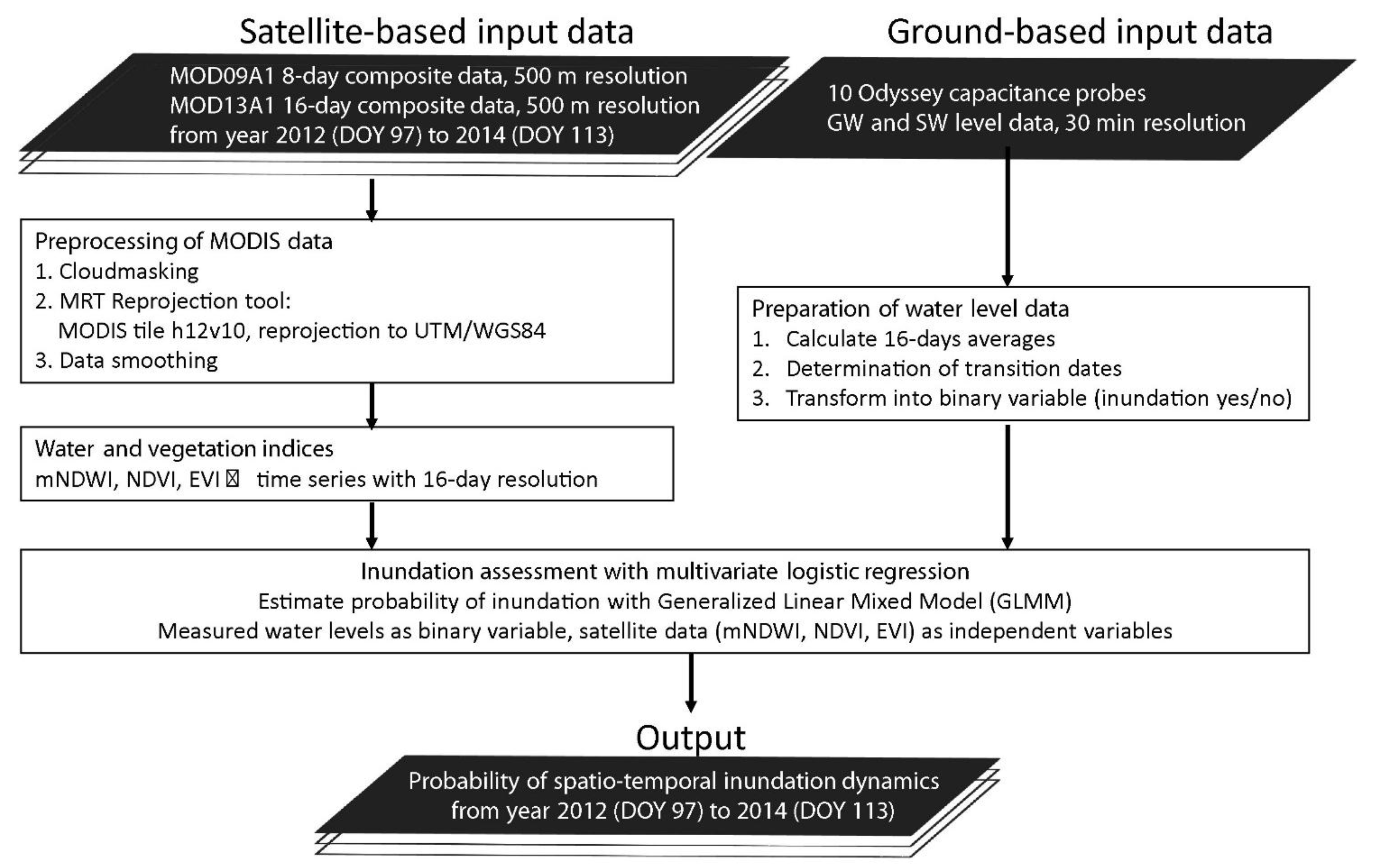
3.1. Space-Based Inundation Assessment

To provide information on the seasonal inundation dynamics from space two different standard MODIS Surface Reflectance Products were obtained. First, the Surface Reflectance 8-day L3 Global 500 m (MOD09A1) product provides 8-day composite images with a resolution of 500 m in the sinusoidal projection. Atmospheric corrections for thin clouds as well as gases and aerosols are implemented already in the downloadable data [50]. MODIS 8-day composites only include pixels with the best quality in terms of highest observation coverage, low view angle, absence of clouds and its shadow as well as aerosol loading [51]. Second, the MODIS Surface Reflectance Product referred to as Vegetation Indices 16-day L3 Global 500 m (MOD13A1) provides 16-day composite images of the Normalized Difference Vegetation Index (NDVI) and the Enhanced Vegetation Index (EVI) with the same spatial resolution and projection. Since problems in inundation mapping often result from the presence of vegetation cover [27], we decided to additionally include these vegetation indices for model building [11,17,52,53]. Time series of both products for the MODIS tile h12v10 were acquired from 1 January 2001 to 30 March 2014 from the Level 1 and Atmosphere Archive and Distribution System (LAABS) run by the National Aeronautics and Space Administration (NASA) Goddard Space Flight Center [54].

All MODIS images were resized to the study area comprising the northern part of the Pantanal (15°–19°S/54.5°–59.5°W, cf. Figure 1a MODIS tile framed in red) and reprojected with the MODIS Reprojection Tool (MRT) to the rectangular projection UTM and the reference system WGS84 [55]. To account for clouds, cloud shadow and the surface reflectance band quality an additional cloud masking was applied for model building using MODIS quality bits.

From MOD09A1 we calculated the widely used modified Normalized Difference Water Index (mNDWI) after Xu [32], which is defined as:

m N D W I = \frac{G R E E N - M I R}{G R E E N + M I R}

(1)

where GREEN is the Green Surface Reflectance Band (545–565 nm) and MIR is the Middle Infrared Band (1628–1652 nm). According to Chen et al. [21], the MOD09A1 band 4 and band 6 are used for calculating the mNDWI, which ranges between −1 (not inundated) and 1 (inundated). From MOD13A1 we used the readily available vegetation indices NDVI and EVI ranging between −1 (no vegetation) and 1 (densely vegetated). To assure the same temporal resolution of all spectral indices, only dates at which all MODIS products were available, were considered. To account for pixel value outliers of the three MODIS products and to include more spatial coherence information a spatial data smoothing was undertaken by calculating the mean value of the surrounding eight pixels for every MODIS pixel averaged by the proper target pixel value.

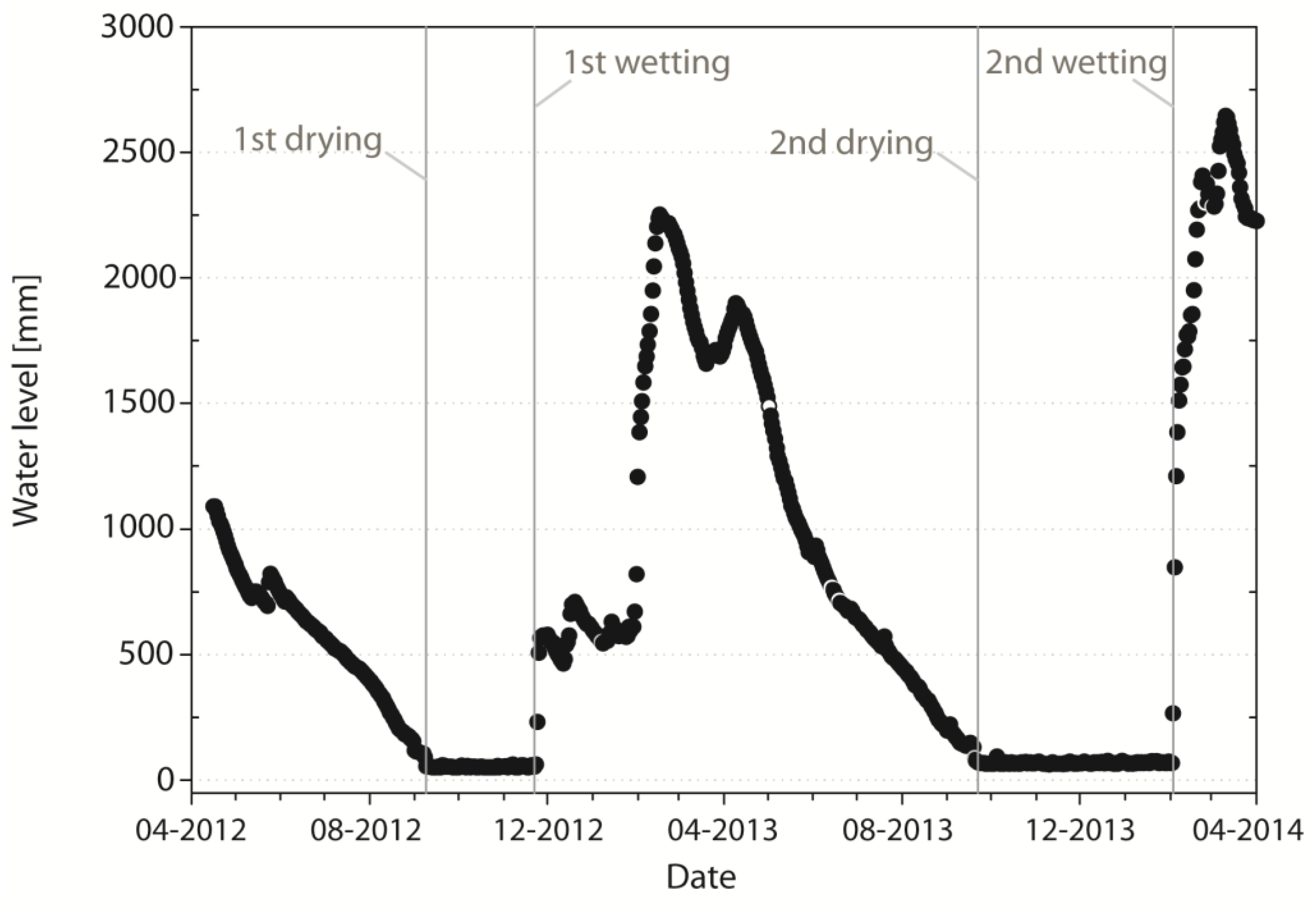
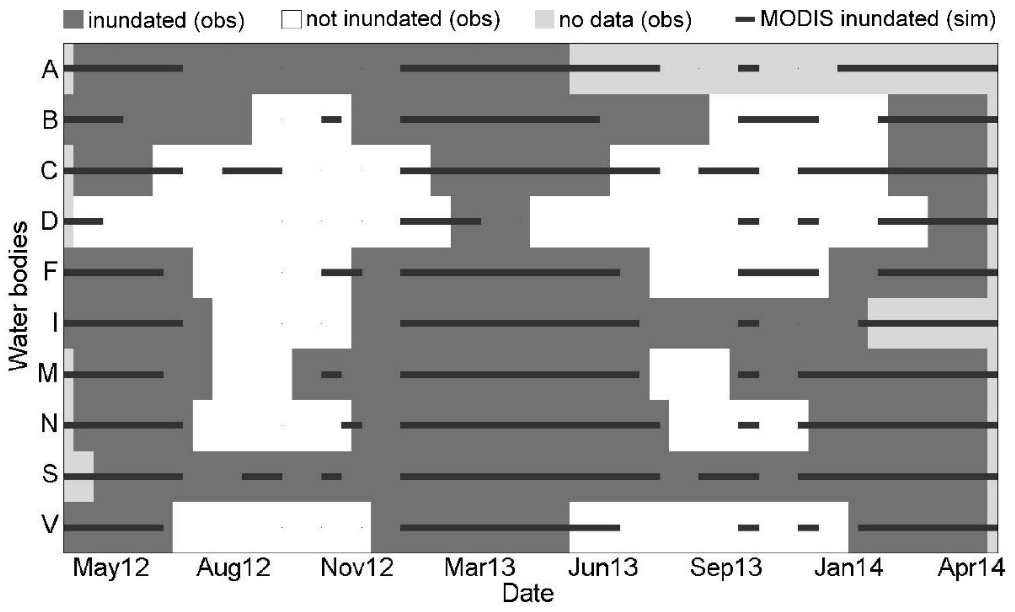
3.2. Ground-Based Inundation Assessment

To determine seasonal inundation dynamics in the field, we used high-resolution water level measurements of surface and groundwater levels recorded every 30 min by Odyssey capacitance probes (Dataflow Systems Ltd., Christchurch, New Zealand) over the two-year study period. Ten water level loggers were installed at different locations in the RPPN (Reserva Particular do Patrimônio Natural: Private reserve of national heritage) SESC (Serviço Social do Comércio: Commercial Social Service) Pantanal, a nature reserve located in the Northern part of the Brazilian Pantanal wetland (Figure 1). The water levels were averaged according to the 16-day temporal resolution of the MODIS products. The transition dates from the wet to the dry seasons (first and second drying during the study period) were determined for the days the water level loggers fell dry and remained dry for at least two weeks (example for location B, Figure 3). The two weeks threshold was chosen to override smaller short-term water level changes. In accordance, the transition dates from the dry to the wet seasons (first and second wetting during the study period) were determined for the days when the water level started to rise after the dry seasons logging water for at least two weeks (Figure 3). Table 1 indicates the location (Figure 1) and type of water body where water-level loggers were installed as well as their transition dates.

Table 1. Location (Figure 1) and type of water body as well as transition dates for the two-year study period (1 April 2012–30 March 2014).

**Table 1.** Location (Figure 1) and type of water body as well as transition dates for the two-year study period (1 April 2012–30 March 2014).
Water Body	Water Body Type	1st Drying	1st Wetting	2nd Drying	2nd Wetting
A	permanent	no drying	no drying	no drying	no drying
B	ephemeral	09.09.2012	23.11.2012	22.09.2013	03.02.2014
C	floodplain	19.06.2012	02.02.2013	26.06.2013	03.02.2014
D	floodplain	no inundation	12.02.2013	25.04.2013	05.03.2014
F	ephemeral	29.07.2012	26.11.2012	24.07.2013	13.12.2013
I	ephemeral	08.08.2012	26.11.2012	no drying	no drying
M	ephemeral	31.07.2012	16.10.2012	27.07.2013	02.10.2013
N	ephemeral	25.07.2012	27.11.2012	15.08.2013	15.12.2013
S	permanent	no drying	no drying	no drying	no drying
V	ephemeral	02.07.2012	11.12.2012	24.05.2013	30.12.2013

Figure 3. Observed water level for water body B (Figure 1) for the study period (1 April 2012–30 March 2014) indicating 1st drying, 1st wetting, 2nd drying and 2nd wetting.

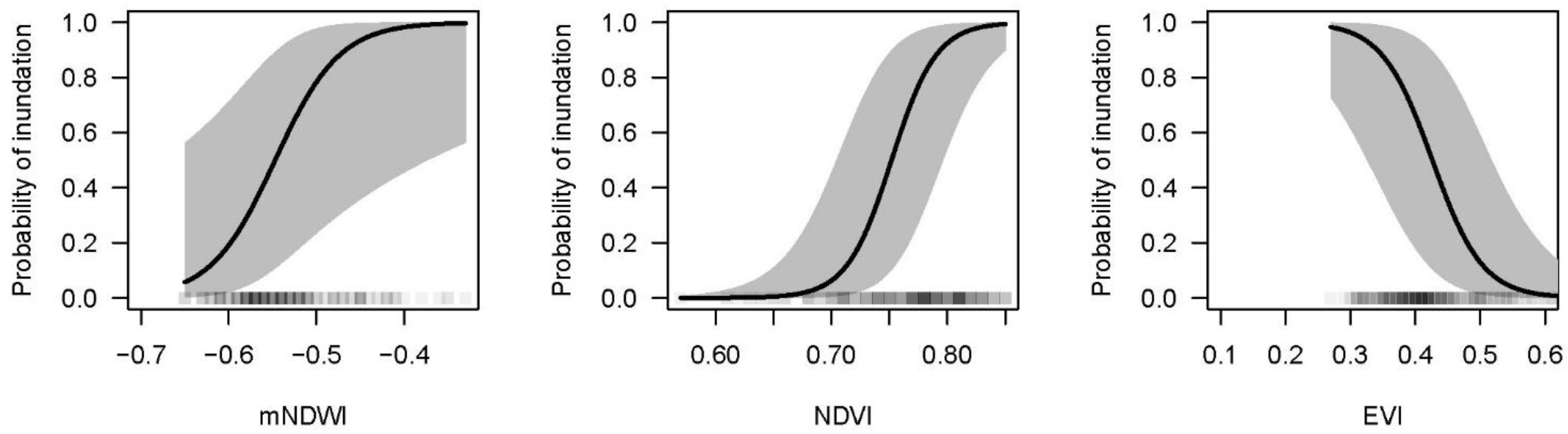
3.3. Multivariate Logistic Regression Model

Fixed thresholds for the spectral indices are often calibrated for separating land from water. Since, in our study, threshold calibration did not lead to reasonable results, we determined the probability of inundation occurrence for all MODIS pixels using a multivariate logistic regression model. It predicts the binary response variable (inundation/no inundation) by the independent variables mNDWI, NDVI and EVI. The water level data measured in the field was recoded to a binary variable, where water levels greater than 15 cm above the surface were set as “flooded” and water levels more than 15 cm below the surface were set as “non-flooded”. This 15 cm threshold is explained by the fact that a water level close to the surface is likely located in a partially flooded pixel due to topographic variability within the pixel [20]. The water level data were separated into training (locations B, C, D, F, N) and testing (locations A, I, M, S, V) datasets. The logistic regression was determined with the training dataset by a Generalized Linear Mixed Model (GLMM) fit by Maximum Likelihood [56]. The fixed term of the model included the three independent variables. To test for absence of collinearity, we calculated the Variance Inflation Factor (VIF), which is commonly used as an indicator for multicollinearity in multiple regression models. All VIFs for each predictor in the GLMM were smaller four, where five is the maximum acceptable value recommended by Rogerson [57]. The pixel ID of the ten pixels, where water levels were derived, was fitted as a random intercept in the mixed model. Parameters of the GLMM (regression coefficients βs, standard errors and confidence intervals) were estimated using the programming language R 3.0.3 [58]. With the GLMM, the probability of inundation could be calculated for every MODIS pixel of all 16-day MODIS composite images.

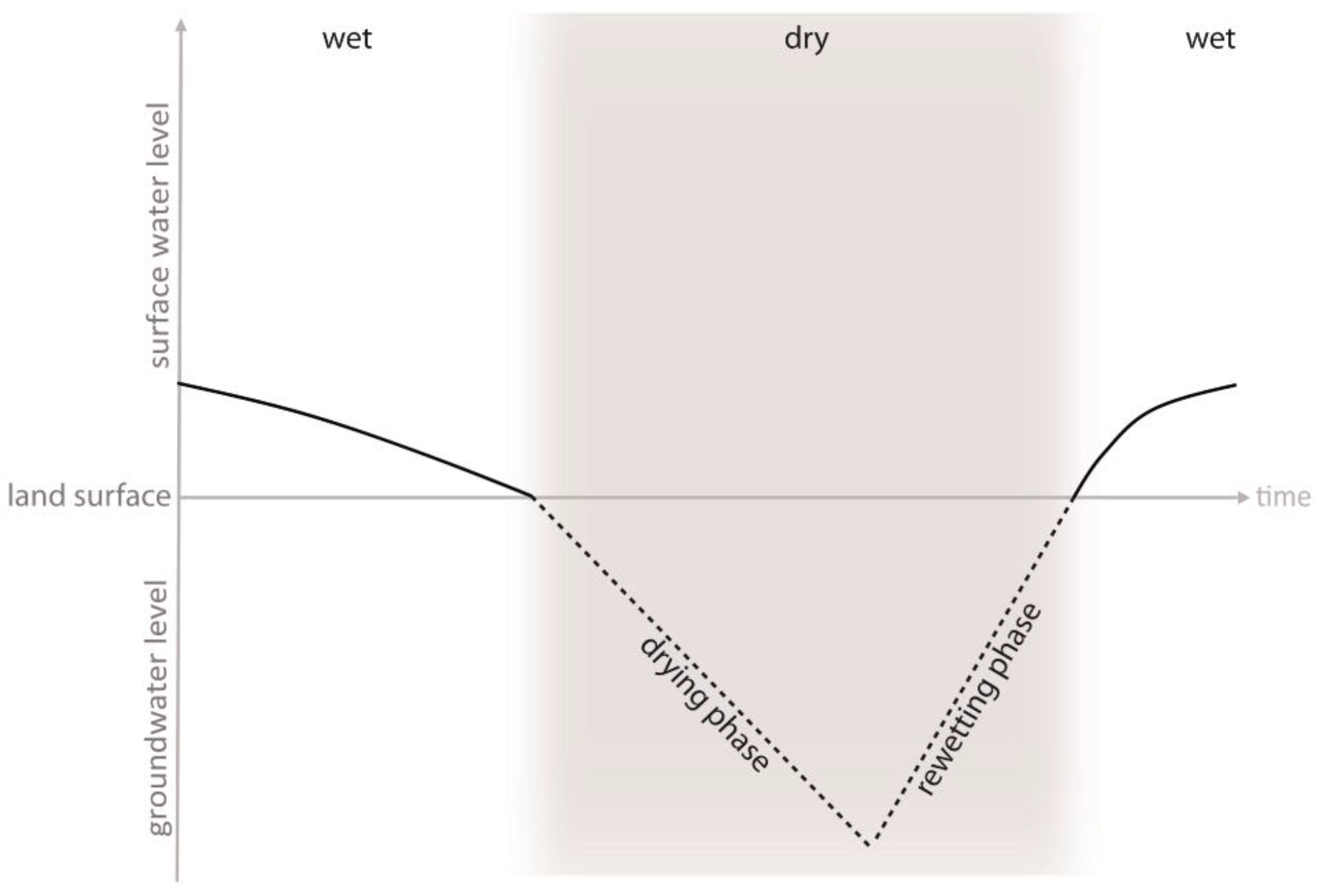
3.4. Dry and Wet Season Delineation for Evaporation Estimation

In order to define the seasonal inundation dynamics for every MODIS pixel, all pixels with estimated probabilities of inundation < 0.5 were defined as “not inundated” and pixels with probabilities of inundation > 0.5 were defined as “inundated” [20,59]. We considered the first transition of a MODIS image indicating inundation to a MODIS image indicating no inundation as the start of the dry season for both years of the study period. The last transition of a pixel indicating no inundation to the pixel indicating inundation determined the end of the dry season. Since inundation duration was determined from MODIS for 16-day periods, we considered the dates in the middle between two consequent MODIS images that showed transitions as the real starting dates for the drying or wetting periods, respectively. This way, we determined the duration of the dry and wet seasons for the two-year study period. Using this water availability information we calculated daily AET with a recently developed approach (short description provided in Appendix 1), where evaporative water loss was simulated on a local scale [16]. Climatic variables used for this approach were derived from the National Institute of Meteorology in Brazil (INMET—Instituto Nacional de Meteorologia) including air temperature, relative humidity, wind velocity, barometric pressure and cloud cover data from OGIMET (www.ogimet.com). To evaluate our approach based on the inundation assessment and the resulting AET rates for the two-year study period we compared AET estimations derived from the satellite-based inundation assessment with the AET results derived from the ground-based inundation assessment. All AET rates were estimated with an independent approach after Schwerdtfeger et al., 2014, using a groundwater evaporation function based on continuous water level measurements in the field (Appendix 1).

3.5. Impact of Local and Upstream Changes

To investigate the impact of local and upstream changes on the ecosystem, we analyzed how AET responded to historic changes in precipitation/wet season precipitation and discharge/wet season discharge. We used precipitation data from the Tropical Rainfall Measuring Mission (TRMM), where the weighted average of the 0.25 degree TRMM cells of the product 3B43 from inside the Cuiabá basin contribution area were used, as well as data of three INMET stations. Discharge data were obtained from the National Water Agency (ANA) network (www.hidroweb.ana.gov.br) for nine different stations (Figure 1, Appendix 2). The prerequisite for a station to be included in our dataset was their data availability of at least seven out of the 13 years (2001 to 2013). In order to find the variable with the largest influence on AET, we related the previously calculated AET rates for the study area for the years 2001 to 2013 to precipitation and discharge data from selected stations. This was done by correlating yearly precipitation data, yearly discharge data of discharge stations and data of discharge losses between all discharge stations with our AET rates. Correlation analysis describes the relationship between two variables, where Pearson’s correlation coefficient (r) ranging between −1 and +1 expresses the strength of this linear relationship. An overview about data used, the data source and the stations is given in Table 2.

Table 2. Data used for investigating the impact of local and upstream changes as well as data source, name of location/station (Figure 1) and detailed data information (MODIS—Moderate Resolution Imaging Spectroradiometer, LAABS—Level 1 and Atmosphere Archive and Distribution System, NASA—National Aeronautics and Space Administration, INMET—Instituto Nacional de Meteorologia: National Institute of Meteorology, ANA—Agência Nacional de Águas: National Water Agency in Brazil, TRMM—Tropical Rainfall Measuring Mission).

**Table 2.** Data used for investigating the impact of local and upstream changes as well as data source, name of location/station (Figure 1) and detailed data information (MODIS—Moderate Resolution Imaging Spectroradiometer, LAABS—Level 1 and Atmosphere Archive and Distribution System, NASA—National Aeronautics and Space Administration, INMET—Instituto Nacional de Meteorologia: National Institute of Meteorology, ANA—Agência Nacional de Águas: National Water Agency in Brazil, TRMM—Tropical Rainfall Measuring Mission).
Data	Data Source	Location/Station	Detailed Data Information
MODIS	LAABS/NASA	Pantanal area inside MODIS tile (Figure 1a, MODIS tile framed in red)	MODIS spectral indices
Meteorological data	INMET	CGB, CAC, RON (Figure 1a, stations labeled in yellow)	Climate variables; Minor data gaps were filled with the weekly moving average of the other years, where data were existent; data of the station closest to each MODIS pixel, respectively, were used.
Precipitation	TRMM	CGB basin (Figure 1a)	Mean precipitation of Cuiabá basin
Precipitation	INMET	CGB, CAC, RON (Figure 1a, stations labeled in yellow)	stations, where at least seven out of the 13 years (2001–2013) of precipitation data were available
Discharge	ANA Hidroweb database	BDB, POE, CGB, BAR, POC, CAC, COR, SFR, POM (Figure 1a,stations labeled in red)	Stations, where at least seven out of the 13 years (2001–2013) of discharge data were available
Discharge loss	ANA Hidroweb database	BDB, POE, CGB, BAR, POC, CAC, COR, SFR, POM	Calculated differences of discharge between stations

4. Results

4.1. Inundation Assessment

Parameters estimated from the GLMM are shown in Table 3. In our study all indices of the logistic regression showed significant p-values (p < 0.01). Thus, they were included in our logistic regression model. The logistic regression was able to predict the probability of inundation with a very high conditional R² (0.84), which is the variance explained by both fixed (three MODIS indices) and random factors (pixel ID).

Index values of the training dataset ranged for mNDWI from −0.65 to −0.33, for NDVI from −0.57 to 0.85 and for EVI from 0.27 to 0.66 (Figure 4). For clarification, all indices correlated positively with inundation alone but in the case of EVI its p-value was not significant and in combination with the other two indices its regression parameter turned negatively. It does not reveal multicollinearity, which has been tested before (cf. Section 3.3) To test the predictability of the regression parameters derived from the GLMM the area under the receiver operating characteristic curve (AUC) as a measure for model discrimination and validation was calculated for the testing dataset, being 0.858. According to the AUC grading guidelines this large AUC credit the model with a “good discrimination” [60].

Table 3. Generalized Linear Mixed Model (GLMM) results (β = regression parameter, SE β = standard error of β, CI = confidential interval, p-value) for all model predictors (mNDWI, NDVI, EVI from MODIS).

**Table 3.** Generalized Linear Mixed Model (GLMM) results (β = regression parameter, SE β = standard error of β, CI = confidential interval, p-value) for all model predictors (mNDWI, NDVI, EVI from MODIS).
Predictor	β	SE β	CI	p-value
Intercept	−13.02	11.082	−1.175	0.2401
mNDWI	27.284	11.93	2.287	<0.01
NDVI	52.043	11.106	4.686	<0.001
EVI	−27.244	6.949	−3.921	<0.001

Figure 4. Probability of inundation for MODIS derived water and vegetation indices (mNDWI, NDVI, EVI) determined by the Generalized Linear Mixed Model (GLMM).

Figure 5. Comparison of ground-based (darkgrey and white boxes) and satellite-based (darkgrey line) inundation assessment for all studied water bodies (Figure 1) over the study period (1 April 2012–30 March 2014).

The inundation dynamics derived from ground- and satellite-based information are compared in Figure 5. The extents of the dry seasons simulated by MODIS data are similar to the observed inundation periods. The inundation determined with MODIS reflects the observed variability to a large extent in terms of inundation duration. Underestimations were found for the floodplain sites (C and D), where the water level loggers observed dry seasons lasting between 224 and 320 days and MODIS determined dry seasons lasting between 96 and 272 days. For most of the ephemeral water bodies (B, F, I, M, N, V) MODIS simulations estimate longer dry periods than observed by the water levels in the field. Obviously, there were no dry seasons observed in the field for the permanent water bodies A and S. The water level logger of water body A was not working properly during the second year of the study period. For both locations (A and S), dry seasons simulated by MODIS were very short. Concerning the overall duration of observed and simulated dry seasons in the study period for all locations we obtained a correlation coefficient of 0.54.

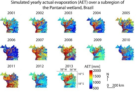
4.2. Evaporation Estimation

For the floodplain water bodies (C and D), yearly AET simulated from the ground-based inundation assessment for the first year of the study period was 1199 and 877 mm, where MODIS driven simulations overestimated AET by 34% and 42%, which corresponds to a difference of 406 and 370 mm, respectively (Table 4). For the second year of the study period MODIS overestimated yearly AET by 38% and 4%, which corresponds to differences in AET of 456 and 27 mm, respectively. For the ephemeral water bodies simulated yearly AET from the ground-based inundation assessment for the first year of the study period ranged from 1510 to 1767 mm. The simulated differences of AET by MODIS ranged from 3% to 29%. Over- and underestimations by MODIS driven simulations of AET could be observed. For the second year of the study period AET rates were simulated from the field-based inundation assessment between 1204 and 1757 mm, where MODIS simulated AET rates ranged from 4% to 22%. For both permanent water bodies (A and S), the simulated yearly AET for the first year of the study period derived from MODIS and the water level loggers were 1543 and 1839 mm, respectively, with a difference of 296 mm. This corresponds to an underestimation of MODIS-derived AET of 16%. For the second year, the differences simulated by MODIS were only 200 and 113 mm for water bodies A and S, respectively. Yearly AET from the ground-based inundation assessment was 1757 mm for both water bodies and 1557 and 1644 mm simulated by MODIS for A and S corresponding to an underestimation of MODIS-derived AET between 11% and 6%. The mean difference of yearly AET for all locations between the ground- and satellite-based inundation assessments was 1.2% (79 mm) for the first and 1.6% (57 mm) for the second year of the study period. The mean simulated daily AET rates for both years of the study period were 3.5 mm/day, ranging from 0.8 to 7.1 mm/day for the first and from 0.6 to 7 mm/day for the second year of the study period. The mean hydroperiod for both years was simulated to last 162 and 160 days, respectively.

The RMSE for the first and the second year of the study period was 296 and 251 mm, the relative RMSE was 19% and 17%, respectively. The predicted AET for the years 2001 to 2013 resulted in mean daily annual AET between 2.4 and 3.7 mm (Table 5) and the mean duration of the hydroperiod ranged from 111 to 197 days averaged over the whole map area (Figure 6). The annual AET ranged from 887 to 1359 mm (Figure 7), where the differences to simulated annual PET rates, ranging from 1541 to 1873 mm, were between 396 and 713 mm. Consequently, simulated AET rates were between 23% and 42% lower than simulated PET rates for the different years.

Table 4. Yearly actual evaporation (AET) [mm] derived from MODIS satellite- and ground-based inundation assessment as well as differences of AET rates [mm and %] for all studied locations (Figure 1) for first (1 April 2012–30 March 2013) and second year (1 April 2013–30 March 2014) of the study period.

**Table 4.** Yearly actual evaporation (AET) [mm] derived from MODIS satellite- and ground-based inundation assessment as well as differences of AET rates [mm and %] for all studied locations (Figure 1) for first (1 April 2012–30 March 2013) and second year (1 April 2013–30 March 2014) of the study period.
1st Year of Study Period	A	B	C	D	F	I	M	N	S	V	Mean
AET [mm] derived from field data	1839	1765	1199	877	1651	1682	1767	1638	1839	1510	-
AET [mm] derived from MODIS	1543	1248	1605	1247	1474	1474	1548	1686	1543	1605	-
Difference [mm]	296	517	−406	−370	177	208	219	−48	296	−96	79
Difference [%]	−16	−29	34	42	−11	−12	−12	3	−16	6	−1.2
2nd Year of Study Period	A	B	C	D	F	I	M	N	S	V	Mean
AET [mm] derived from field data	1757	1546	1188	754	1521	1757	1724	1581	1757	1204	-
AET [mm] derived from MODIS	1557	1227	1644	781	1304	1371	1607	1644	1644	1439	-
Difference [mm]	200	319	−456	−27	216	386	118	−63	113	−235	57
Difference [%]	−11	−21	38	4	−14	−22	−7	4	−6	19	−1.6

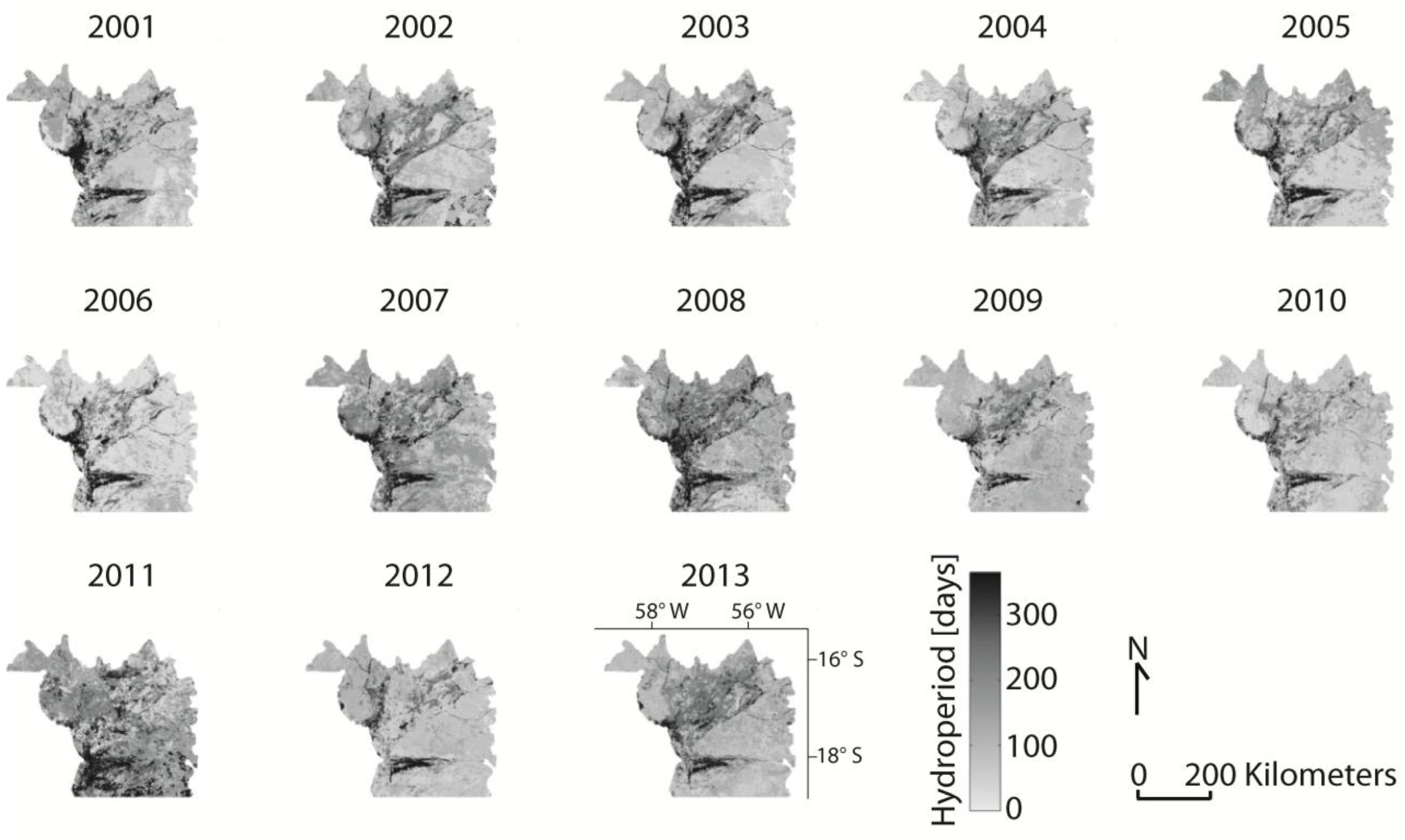
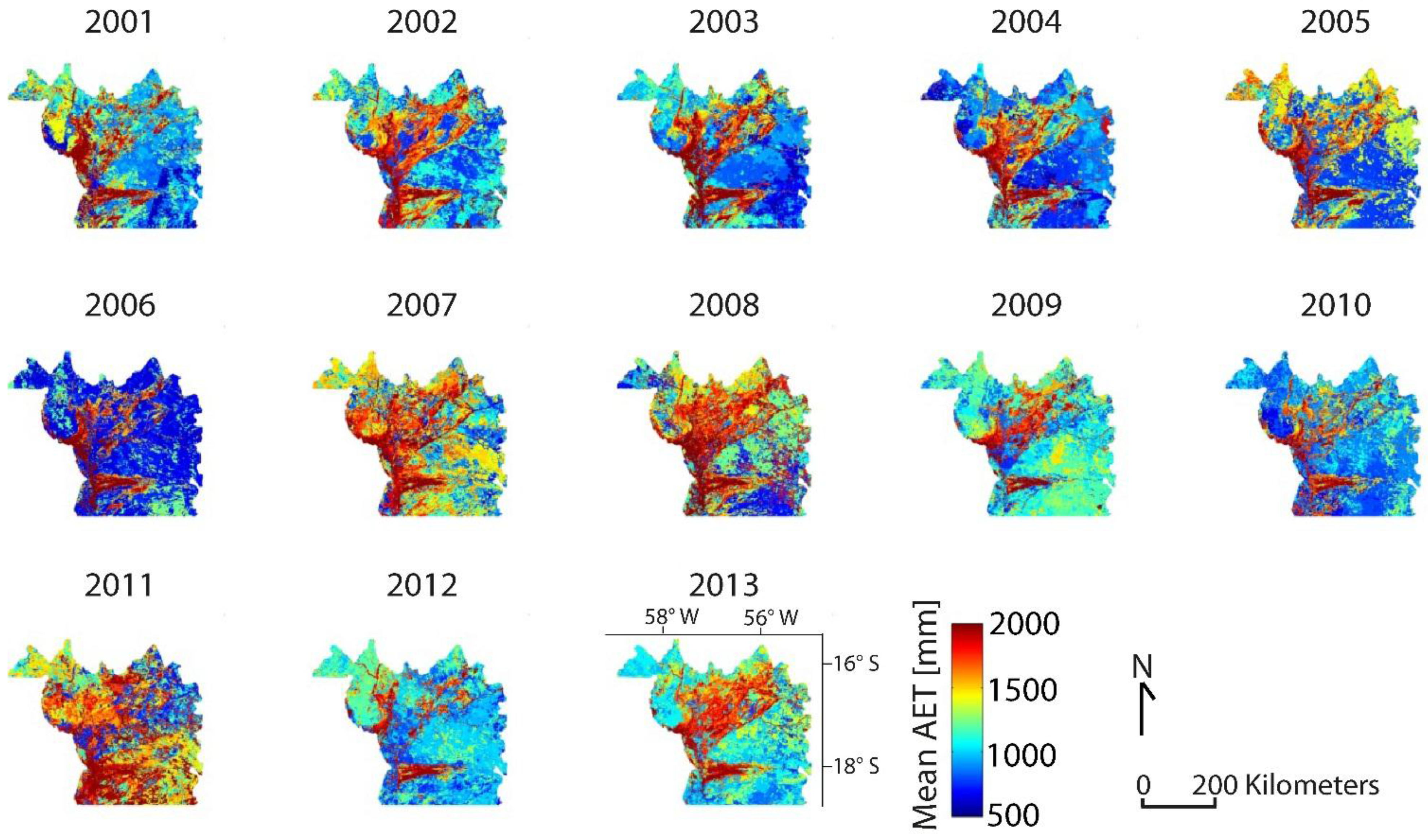
Table 5. Simulated mean hydroperiod, daily and yearly mean of actual evaporation (AET), yearly mean of potential evaporation (PET), the difference of yearly AET and PET as well as the ratio of AET and PET for the years 2001 to 2013.

**Table 5.** Simulated mean hydroperiod, daily and yearly mean of actual evaporation (AET), yearly mean of potential evaporation (PET), the difference of yearly AET and PET as well as the ratio of AET and PET for the years 2001 to 2013.
Year	Mean Hydroperiod [days]	AET Daily Mean [mm]	AET Yearly Mean [mm]	PET Yearly Mean [mm]	PET-AET [mm]	AET/PET [–]
2001	142	2.9	1066	1604	538	0.66
2002	149	3.1	1116	1630	514	0.68
2003	149	2.9	1051	1574	523	0.67
2004	132	2.7	993	1578	585	0.63
2005	151	3.0	1091	1580	490	0.69
2006	111	2.4	887	1541	654	0.58
2007	175	3.4	1223	1652	429	0.74
2008	180	3.4	1258	1690	432	0.74
2009	141	3.1	1146	1681	535	0.68
2010	118	3.0	1110	1823	713	0.61
2011	197	3.7	1359	1756	396	0.77
2012	128	3.3	1210	1873	664	0.65
2013	157	3.5	1260	1778	518	0.71
min	111	2.4	887	1541	396	0.58
max	197	3.7	1359	1873	713	0.77

Figure 6. Simulated hydroperiods [days] for the years 2001 to 2013, where the map area corresponds to the Pantanal area located inside the MODIS tile (Figure 1a).

Figure 7. Simulated yearly means of actual evaporation (AET) [mm] for the years 2001 to 2013, where the map area corresponds to the Pantanal area located inside the MODIS tile (Figure 1a).

4.3. Impact of Local and Upstream Changes

For one precipitation station (CGB) simulated AET was positively correlated with annual and wet season precipitation (Table 6 and Table 7). For all other stations, the correlations were negative ranging from −0.22 to −0.17 for yearly precipitation and from −0.26 to 0 for wet season precipitation. Corresponding p-values were significant at the 5% level for yearly precipitation data for all stations except for CAC and for the wet season precipitation only for TRMM. Only one (COR) out of nine discharge stations showed a positive correlation with simulated AET for the whole map area (Figure 7). Correlations for all other discharge stations were between −0.35 and −0.08. All p-values were significant at the 5% level. For the wet season, discharge data of two additional discharge stations (SFR, POM) were positively correlated with simulated AET with significant p-values at the 5% level. Correlations between wet season discharge and simulated AET for all other discharge stations ranged from −0.25 to −0.05. Yet significant p values at the 5% level were only found for some stations. We found seven out of twelve river sections with positive correlations between their discharge loss and simulated AET with significant p values. For the Cuiabá River stations (Figure 1a) positive correlations between their discharge loss and simulated AET were between 0.38 and 0.82. Correlations between the discharge loss of the two Paraguay River sections BDB-SFR as well as BDB-POM and simulated AET were between 0.48 and 0.65. Correlations between discharge at all other river sections with simulated AET ranged from −0.29 to −0.04 with significant p-values at the 5% level.

Table 6. Correlation coefficients (r) between precipitation (P) or discharge (Q) and simulated actual evaporation (AET) as well as correlation coefficients (r_wet) between wet season precipitation or wet season discharge and simulated AET and their p-values for considered INMET (Instituto Nacional de Meteorologia: National Institute of Meteorology) and Hidroweb stations from ANA (Agência Nacional de Águas: National Water Agency in Brazil) in the study area (Figure 1a).

**Table 6.** Correlation coefficients (r) between precipitation (P) or discharge (Q) and simulated actual evaporation (AET) as well as correlation coefficients (r_wet) between wet season precipitation or wet season discharge and simulated AET and their p-values for considered INMET (Instituto Nacional de Meteorologia: National Institute of Meteorology) and Hidroweb stations from ANA (Agência Nacional de Águas: National Water Agency in Brazil) in the study area (Figure 1a).
	TRMM P	CGB P	CAC P	RON P	CGB Q	BAR Q	POC Q	COR Q	BDB Q	POE Q	CAC Q	SFR Q	POM Q
r	−0.17	0.47	−0.18	−0.22	−0.34	−0.16	−0.20	0.83	−0.35	−0.31	−0.33	−0.18	−0.08
p	0.00	0.00	0.27	0.01	0.00	0.00	0.00	0.00	0.00	0.00	0.00	0.00	0.00
r_wet	−0.07	0.56	0.00	−0.26	−0.24	−0.05	−0.25	0.88	−0.15	−0.19	−0.18	0.43	0.61
p_wet	0.00	0.27	0.08	0.83	0.65	0.00	0.00	0.00	0.00	0.00	0.29	0.00	0.00

Table 7. Correlation coefficients (r) between annual discharge loss (Q_loss) or wet season discharge loss (Q_lossW) and simulated actual evaporation (AET) for the study area and their p-values for considered Hidroweb stations from ANA (Agência Nacional de Águas: National Water Agency in Brazil) in the study area (Figure 1a).

**Table 7.** Correlation coefficients (r) between annual discharge loss (Q_loss) or wet season discharge loss (Q_lossW) and simulated actual evaporation (AET) for the study area and their p-values for considered Hidroweb stations from ANA (Agência Nacional de Águas: National Water Agency in Brazil) in the study area (Figure 1a).
	CGB-BAR Q_loss	CGB-BAR Q_lossW	CGB-POC Q_loss	CGB-POC Q_lossW	BDB-POE Q_loss	BDB-POE Q_lossW	BDB-CAC Q_loss	BDB-CAC Q_lossW	BDB- SFR Q_loss	BDB- SFR Q_lossW	BDB- POM Q_loss	BDB- POM Q_lossW
r	0.69	0.38	0.82	0.55	0.37	−0.06	−0.29	−0.14	−0.15	0.48	−0.04	0.65
p	0.00	0.00	0.00	0.00	0.00	0.00	0.00	0.00	0.01	0.01	0.00	0.00

5. Discussion

5.1. Use of MODIS and Remotely Sensed Indices

We used MODIS 16-day composite images instead of daily products since frequent cloud cover in tropical regions makes it difficult to use the daily products. It is obvious that these composite images cannot provide a very detailed inundation assessment but are sufficient to characterize the hydrological flooding regime. Several studies demonstrate the usefulness of MODIS composite images to study hydrological conditions in wetlands [20,23]. Chen et al. [22] compared the ability of daily and 8-day MODIS composites images for inundation mapping. They summarize that both products provide a reasonable accuracy at a regional scale. After Chen et al. [21], the observation frequency provides sufficient cloud free 8-day MODIS composites during the flooding period.

Choosing the mNDWI for delineating water from land for our study is based on the fact that the mNDWI was already successfully used to study inundation dynamics with MODIS time series [21,29]. Ji et al. [14] recommend using the mNDWI for mapping surface water because it has lower influence of subpixel vegetation components compared to others. During calibration of a fixed index threshold for separating land from water we obtained unsatisfying results. Therefore we used the logistic regression. Its advantage is that it can be directly validated and its value for binary classification was proved by Ordoyne and Friedl [20]. Combining the mNDWI with the vegetation indices the logistic regression results demonstrate the successful combination of our index composition. A combination of MODIS indices to detect flooding was also successfully used by Xiao et al. [35] in paddy rice fields in Asia.

In general, a broad range of index values for determining inundation can be found in the literature, which highlights the necessity of thoroughly calibrating thresholds for every study area with its specific characteristic. The large confidence interval of the mNDWI (Figure 4) shows that the water index alone is not a sufficient predictor for inundation mapping. Its value is strongly altered as a function of green vegetation cover. We deduce that only the combination of using different indices, one or more being more sensible to water surface extent and others to green vegetation cover, can separate land from water with reasonable results. The high conditional R² (0.84) supports our index combination and the effective estimation of inundation probability with our approach.

5.2. Inundation Assessment

We are aware of the limited representativeness of our water level probes in terms of spatial resolution and different vegetation forms in the Pantanal. However, to our knowledge our water level measurements are the only high-resolution dataset with continuous two-year time series of water levels at several locations inside the northern Pantanal, which make them a valuable data source for assessing the ecosystem’s state. Using satellite information is crucial especially in remote areas, where usually no other long-term inundation monitoring is available [28], but these data sources need ground-based information. Considering lack of reliable data in our study area, we made use of existing data but are conscious about the fact that a two-year time series of water levels are not sufficient to address all variability in seasonal inundation dynamics. However, since studies that examine MODIS satellite imagery with gauged hydrological data are very scarce for the Pantanal wetland, we considered our correlation between ground- and satellite-based inundation assessment (r = 0.54) sufficient to proceed with our analysis. Pavelsky and Smith [36] compared observed water levels and inundation patterns derived from MODIS in the Peace-Athabasca Delta in Canada and obtained correlation coefficients for four different sites between 0.33 and 0.94. Thakur et al. [61] compared annual NDVI values from MODIS with measured annual mean groundwater levels in two Turkish wells and obtained correlation coefficients of 0.31 and 0.74, where the lower value was probably due to variation in terrain height. Ordoyne and Friedl [20] evaluated their logistic model with independent sites in the Everglades and state that the overall pattern was realistic but showed considerable model errors. Only few studies exist that evaluate MODIS time series with observed data in the field. Some of them use additional information, such as the information given by a DEM in the study of Peng et al. [53]. Li et al. [34] derived water levels by subtracting ground elevation from water surface elevation.

For defining the dry season we considered only the first and last MODIS images that determined the transitions from the dry to the wet seasons and vice versa. This implies that the inundation process of a seasonal wetland does usually not show smaller short-term periods with inundation during the dry season, since its flood pulse is defined as monomodal [42]. We attribute the short-term increase of the probabilities of inundation within the dry season to model weaknesses, which are explained below (Section 5.4). In our study, inundation duration of the permanent water bodies and also of most of the ephemeral water bodies was underestimated by MODIS. A general trend of underestimating inundation by MODIS was also observed by Chen et al. [22]. In contrast, the inundation duration at our floodplain sites were overestimated by MODIS. A possible reason could be that inundation with small water depth, given in floodplain sites, is always more susceptible to misclassification than with deep water levels [22].

5.3. Evaporation Estimation

At locations without inundation, we simulated dry season AET rates between 0.3 and 2.3 mm/day for the years 2001 to 2013, which are very similar to the dry season AET rates for a Brazilian floodplain ranging from 1.3 to 3.3 mm/day [62]. Hutley et al. [63] report AET rates from 1.2–1.9 mm/day from the mid to the late dry season in a wet–dry Australian savanna. The resulting annual AET between 427 and 694 mm corresponds well with our minimum simulated yearly AET rates ranging from 557 to 693 mm. Daily mean AET determined for the northern Pantanal with the Bowen ratio method ranged from 2.5 mm in the dry season to 4 mm/d in the wet season [64]. These values correspond well to our mean daily AET rates ranging from 2.4 to 3.7 mm for the years 2001 to 2013. That range is due to the simulated water availability as well as the available energy for evaporation. Sanches et al. [64] also report a difference of AET to open water evaporation, which was 30% and 25% lower for the dry and the wet season, respectively. This reduction is in correspondence to our findings, where AET is between 23% and 42% lower than PET for the years 2001 to 2013. In addition, their annual AET of 1208 mm and PET of 1557 mm for the year 2007, derived from micrometeorological measurements at location C in our study area, corresponds well to our simulation of 1223 and 1652 mm for the year 2007. Comparing evaporation results from the satellite-based inundation assessment with evaporation results based on inundation measurements of our approach reveals that it provides reasonable evaporation estimations for the Pantanal wetland.

5.4. Model Weaknesses and Description of Uncertainties

An important issue regarding model uncertainties results from the scale effect between local and space-born observations. While water level data are point measurements, spectral indices from remote sensing represent areas according to the system’s spatial resolution. When using these ground truth data for model building and validating the MODIS inundation prediction, it introduces a systematic error to the approach [65]. However, in our study area, we were dependent on that small-scale information since no other data were available for evaluating our approach. Model weaknesses probably result from the fact that in our study one water level probe is compared with a pixel of 500 m resolution. The Pantanal is a difficult-to-access area and during installation we could not guarantee that the water level probes represent the mean pixel elevation. This was also one reason for model errors in the study of Ordoyne and Friedl [20]. Therefore, we followed their approach by only labeling sites as flooded, when the water level was above 15 cm (and as non-flooded, when the water level was below 15 cm) to minimize model bias. Huang et al. [18] explained that the timing of the observed flooding in relation to MODIS-derived inundation is offset due to the relative gauge position.

Another source of uncertainty results from the fragmentation and subpixel heterogeneity in one MODIS pixel [35]. It limits the detection of smaller water bodies inside of a pixel [22]. The very diverse landscape of the Pantanal wetland is therefore difficult to cover in one pixel value. Especially images from seasonal transition times are susceptible to misclassification, since water bodies in the study area dry out heterogeneously inside of a pixel. The determination of pixels, which are covered by vegetation mixed with or completely flooded by water, is usually difficult [30,33]. Pixels can be covered by a mixture of different land types, which are all combined in one index pixel value leading to an over- or underestimation of MODIS-derived inundation [30].

Sakamoto et al. [17] pointed out that under dense vegetation cover it is usually difficult to detect flooded areas with MODIS. Inundation is more likely detected when plants are submerged by rising water levels in the pixel, which increases the ratio of water area to vegetation cover. Vegetation such as high tree cover contributes to the error by masking the signal detected by MODIS [20]. This was eventually the case for location D, where a large forest stand (V. divergens), locally called Cambarazal, covers the area [64]. The use of a multispectral index for separating land from water cannot guarantee the detection of inundation beneath vegetation cover and at the same time distinguish between inundation and dark soil (Chen et al. 2013). Landmann et al. [33] sum up that besides inherent pixel variability and mapping errors, the variation in high water and vegetation dynamics tend to be responsible for inaccuracies in mapping wetland dynamics. They also mention the variability of aquatic vegetation cover in space and time. Despite the low spatial resolution of the MODIS pixels that results in a large heterogeneity of pixel compositions, dos Santos et al. [66] conclude that MODIS provide satisfactory results in mapping the dynamics of the Pantanal biome.

5.5. Impact of Local and Upstream Changes

The correlation between simulated AET and the discharge is determined empirically in our study. The human impact on inundation in our study is assumed based on a thorough literature review. Freshwater wetlands such as the Pantanal are stated to be among the most threatened ecosystems on earth [67]. They are especially vulnerable to human-induced activities such as land use change or dam construction [68,69] in the upstream watersheds. In the Pantanal region, hydropower plants were constructed to cope with the increasing electricity needs affecting intensively the natural discharge of Pantanal tributaries and their water levels. As a result, the initiation of the flooding process in the wetland is also changed [8]. Furthermore, Brazil is the second largest soybean producer in the world. Large parts of its territory are used to plant this water-intensive crop [70]. This is also the case for Mato Grosso, in which 65% of the Pantanal area is located [71], where water for soybean irrigation is taken from Pantanal tributaries [70]. Therefore, it is highly probable that human activity in the upper catchments changes the inflow conditions in the wetland as well, and thus also influences AET. We found primarily negative correlations between precipitation and simulated AET, which can be explained by the fact that in years with higher precipitation simulated AET is lower due to the cloud cover inhibiting radiation to reach the ground surface. This radiation reduction results in a lower AET since in the tropics radiation is the main factor controlling AET [72]. It is not surprising that most of the positive, strong correlations (0.38 < r < 0.82) were found between the discharge loss and the simulated AET. Evaporation is considered to be the dominant cause of water loss from seasonal wetlands [73]. However, there are differences among the wetlands. The positive correlations between the discharge loss and the simulated AET reveal that the inundation dynamics, which are assumed to be a result of man-made impacts on upstream inflow to the wetland (through hydropower plant reservoirs or land use change), strongly determine AET in the wetland. Our results indicate that the Pantanal wetland is more susceptible to changes in tributary inflows than to changes in local precipitation, which is determined by the regional climate conditions [74]. The direct effect of human-induced changes on the inundation dynamics, and thus on the evaporative water loss, will have major implications for the wetland ecosystem recalling that the annual flood pulse is the key driver for the wetland’s biodiversity [5]. Using evaporation as a proxy for the ecosystem functioning is based on the link it constitutes between the climatological and the ecological system and its important role in the hydrological water cycle [6]. We are aware that our study is only based on thirteen years of data and thus our results can only be seen as a first step in investigating the impact of local and upstream changes on the wetland system.

6. Conclusions

The aim of our study was developing an approach to estimate regional evaporation for remote wetland areas taking into account the inundation dynamics and to investigate the impact of local and upstream changes on the ecosystem. We were able to determine inundation dynamics of wet and dry seasons for the Pantanal study area using MODIS water and vegetation indices. A unique dataset of continuous 2-year time series of water levels at several locations inside the northern Pantanal served to evaluate the inundation dynamics. We obtained a correlation coefficient of 0.54 for the overall duration of observed and simulated dry seasons in the study period for all locations. We found that MODIS data can be used to characterize the hydrological flooding regime in the remote Pantanal wetland area even though different sources of uncertainty limit a too detailed interpretation. For instance, the MODIS derived inundation did not reflect all the observed variability in terms of inundation duration. With our results, we can state that satellite information is a valuable data source for remote wetland areas but only when representative ground truthing data is available.

Using the information about inundation dynamics, which determine the available water for evaporation, it was possible, for the first time, to estimate regional AET for the Pantanal with a process-based evaporation model. AET estimations ranged from 877 to 1839 mm for the first year of the study period and from 745 to 1757 mm for the second year of the study period, where the MODIS derived estimations were between 1247 and 1686 mm as well as 781 and 1644 mm, respectively. This corresponds to a relative RMSE of 19% and 17%. In order to assess the impact of local and upstream changes on the Pantanal ecosystem, we calculated AET for the years 2001–2013 and applied a correlation analysis that related our evaporation results to the local precipitation and inflow of tributaries. The highest correlations were found between discharge loss and simulated AET for seven stations inside of the Pantanal ranging from 0.38 to 0.82. This indicates that the Pantanal wetland is more susceptible to changes in tributary inflows than to changes in local precipitation determined by the regional climate conditions. Our approach may serve as a first step to investigate the Pantanal ecosystem’s state. It reveals that further research is indispensable to assess to which extent the Brazilian Pantanal wetland is vulnerable to man-made impacts on the inundation process due to upstream land use modifications. Hence, future research requires further long-term monitoring desirably with a higher sampling resolution.

Until today, tropical wetlands are not yet well considered in global climate and land cover products. Knowing that tropical wetlands are not only valuable biodiversity hotspots but are determinant for regional up to continental climate conditions underline the importance of an accurate representation in large-scale hydrological models in order to improve their predictability.

Acknowledgments

The MODIS data used in this study were acquired as part of NASA’s Earth-Sun System Division, archived and distributed by the MODIS Adaptive Processing System (MODAPS). The authors are grateful to the RPPN SESC Pantanal for transport, accommodation and field assistance in the framework of the Long Term Ecological Research project with funding through the Brazilian National Science and Technology Research Council (Conselho Nacional de Desenvolvimento Científico e Tecnológico—CNPq) launched by E.G. Couto. Field study was assisted by the “guarda-parques” and “brigadistas” from the RPPN SESC Pantanal, where especially the help of Guarda-Parques Rodrigo and Pedro Paulo is acknowledged. Meteorological data has been collected from INAU, the Brazilian National Research Institute for Humid Areas (Instituto Nacional de Ciência e Tecnologia em Áreas Úmidas). The first author was funded by the IPSWaT (International Postgraduate Studies in Water Technology) PhD scholarship of the German Federal Ministry of Education and Research (BMBF). We acknowledge statistical advice on GLMM of Simone Ciuti.

Author Contributions

Julia Schwerdtfeger planned and set-up the fieldwork in the Pantanal wetland, collected the data and wrote the manuscript. Sérgio Gripp conducted the cloud masking of the satellite images. All authors contributed to the data analysis, evaluation and interpretation and all co-authors reviewed the manuscript.

Appendix 1: Calculation of Daily AET Based on Water Availability after Schwerdtfeger et al. (2014)

To calculate AET based on water available determined by the seasonal inundation dynamics of the study area, the Turc model modified for subtropical regions [75,76] was chosen to calculate PET for different locations in the study area. The PET model results were used to estimate AET rates by applying the groundwater evaporation function after Stoll and Weiler [77]. This function uses continual in situ measurements of surface- and groundwater levels to predict AET based on the relationship between AET and groundwater depth. During the inundation times, AET is PET. Simulated AET was evaluated for one location with observations from a Bowen ratio climate station inside of the study area obtained from Sanches et al. (2011), where the Bowen ratio method measures the latent heat flux in the energy balance including all evaporating fluxes such as evaporation and transpiration. To transfer the model results to different locations, where measured groundwater levels were not available, a general drying and rewetting approach was developed using measured data of one groundwater probe in the study area (Figure A1). Their measured groundwater levels served to determine a general procedure of drying and wetting assuming these processes to be consistent in time and space. The drying phase started from the first decrease in groundwater levels to the lowest groundwater level measured in the dry season. From there, rising groundwater levels determined the rewetting phase up to the date where they reached again the land surface. For both phases linear regressions were calculated and validated with data of a second groundwater probe. The regression-derived groundwater levels were transferred to locations without groundwater level measurements by shifting the drying and rewetting phases with their specific slopes based on the duration without inundation. For the application of this approach, only the starting and ending dates of the dry season are necessary. This way, groundwater levels can be calculated on a regional scale as well as for locations without measured groundwater levels to determine the water available for evaporation.

Figure A1. Conceptual model of the drying and rewetting approach modified from [16].

Appendix 2: Time Series of Data Used for Investigating Impact of Local and Upstream Changes

Table A1. Yearly precipitation and wet season precipitation (October–March, subscript wet) obtained from TRMM (Tropical Rainfall Measuring Mission) and INMET (Instituto Nacional de Meteorologia: National Institute of Meteorology) stations (Figure 1a, stations labeled in yellow, CGB—Cuiabá, CAC—Cáceres, RON—Rondonópolis) for the years 2001 to 2013.

**Table A1.** Yearly precipitation and wet season precipitation (October–March, subscript wet) obtained from TRMM (Tropical Rainfall Measuring Mission) and INMET (Instituto Nacional de Meteorologia: National Institute of Meteorology) stations (Figure 1a, stations labeled in yellow, CGB—Cuiabá, CAC—Cáceres, RON—Rondonópolis) for the years 2001 to 2013.
Year	TRMM [mm]	TRMM_wet [mm]	CGB [mm]	CGB_wet [mm]	CAC [mm]	CAC_wet [mm]	RON [mm]	RON_wet [mm]
2001	1815	1453	1226	1073	1292	1131	1137	926
2002	1671	1354	1173	988	974	744	1214	1151
2003	1772	1470	1372	1113	1094	948	1290	1016
2004	1696	1465	1177	967	1136	914	1396	1178
2005	1510	1299	967	829	1199	1088	1246	1120
2006	1773	1485	1518	1193	1404	1175	1528	1379
2007	1613	1444	1604	1404	1283	1161	1250	1091
2008	1594	1320	no data	no data	1326	1198	1527	1193
2009	1849	1438	no data	no data	1255	987	1443	1216
2010	1443	1335	1597	1474	1347	1211	1283	1206
2011	1755	1567	1673	1467	1230	1120	1147	1103
2012	1670	1243	1620	1231	981	817	1514	1225
2013	1659	1425	1525	1322	1091	905	1300	1111
min	1443	1243	967	829	974	744	1137	926
max	1849	1567	1673	1474	1404	1211	1528	1379

Table A2. Yearly mean discharge of Hidroweb stations from ANA (Agência Nacional de Águas: National Water Agency in Brazil) (Figure 1a, stations labelled in red, CGB—Cuiabá, BAR—Barão de Melgaço, POC—Porto Cercado, COR—Rio Correntes, BDB—Barra do Bugres, POE—Porto Estrela, CAC—Cáceres, SFR—São Francisco, POM—Porto da Manga) for the years 2001 to 2013.

**Table A2.** Yearly mean discharge of Hidroweb stations from ANA (Agência Nacional de Águas: National Water Agency in Brazil) (Figure 1a, stations labelled in red, CGB—Cuiabá, BAR—Barão de Melgaço, POC—Porto Cercado, COR—Rio Correntes, BDB—Barra do Bugres, POE—Porto Estrela, CAC—Cáceres, SFR—São Francisco, POM—Porto da Manga) for the years 2001 to 2013.
Year	CGB [m³/s]	BAR [m³/s]	POC [m³/s]	COR [m³/s]	BDB [m³/s]	POE [m³/s]	CAC [m³/s]	SFR [m³/s]	POM [m³/s]
2001	238	243	251	91	119	150	497	1264	1443
2002	433	439	390	97	159	195	587	1748	2066
2003	420	453	388	95	182	213	612	1701	2009
2004	396	389	349	88	141	165	510	1502	1742
2005	309	345	332	60	108	135	462	1330	1499
2006	497	498	428	17	178	214	628	1928	2225
2007	321	381	383	296	140	180	558	1756	2128
2008	419	455	no data	no data	134	no data	516	no data	no data
2009	no data	402	no data	no data	130	no data	435	no data	no data
2010	no data	390	no data	no data	178	no data	542	no data	no data
2011	368	407	no data	no data	148	no data	544	no data	no data
2012	273	318	no data	no data	100	no data	394	no data	no data
2013	356	380	no data	no data	no data	no data	no data	no data	no data
min	238	243	251	17	100	135	394	1264	1443
max	497	498	428	296	182	214	628	1928	2225

Table A3. Mean of maximum discharge (Dec-Apr) of Hidroweb stations from ANA (Agência Nacional de Águas: National Water Agency in Brazil) (Figure 1a, stations labelled in red, CGB—Cuiabá, BAR—Barão de Melgaço, POC—Porto Cercado, COR—Rio Correntes, BDB—Barra do Bugres, POE—Porto Estrela, CAC—Cáceres, SFR—São Francisco, POM—Porto da Manga) for the years 2001 to 2013.

**Table A3.** Mean of maximum discharge (Dec-Apr) of Hidroweb stations from ANA (Agência Nacional de Águas: National Water Agency in Brazil) (Figure 1a, stations labelled in red, CGB—Cuiabá, BAR—Barão de Melgaço, POC—Porto Cercado, COR—Rio Correntes, BDB—Barra do Bugres, POE—Porto Estrela, CAC—Cáceres, SFR—São Francisco, POM—Porto da Manga) for the years 2001 to 2013.
Year	CGB [m³/s]	BAR [m³/s]	POC [m³/s]	COR [m³/s]	BDB [m³/s]	POE [m³/s]	CAC [m³/s]	SFR [m³/s]	POM [m³/s]
2001	847	569	448	118	301	335	989	1287	1503
2002	1385	919	583	133	458	519	1174	1962	1957
2003	1157	870	577	127	494	501	1189	1478	1504
2004	1031	831	565	118	356	391	1010	1426	1555
2005	1039	825	552	101	343	377	989	1404	1646
2006	1447	986	649	41	467	516	1214	1735	1730
2007	907	781	597	277	372	437	1184	2094	2205
2008	1275	938	no data	no data	420	no data	1036	no data	no data
2009	no data	829	no data	no data	371	no data	795	no data	no data
2010	no data	849	no data	no data	485	no data	1208	no data	no data
2011	1196	890	no data	no data	441	no data	1156	no data	no data
2012	729	656	no data	no data	229	no data	675	no data	no data
2013	1057	898	no data	no data	no data	no data	no data	no data	no data
min	729	569	448	41	229	335	675	1287	1503
max	1447	986	649	277	494	519	1214	2094	2205

Conflicts of Interest

The authors declare no conflict of interest.

References

Gopal, B. Perspectives on wetland science, application and policy. Hydrobiologia 2003, 490, 1–10. [Google Scholar] [CrossRef]
Keddy, P.A.; Fraser, L.H.; Solomeshch, A.I.; Junk, W.J.; Campbell, D.R.; Arroyo, M.T.K.; Alho, C.J.R. Wet and wonderful. The world’s largest wetlands are conservation priorities. Bioscience 2009, 59, 39–51. [Google Scholar] [CrossRef] [Green Version]
Junk, W.J.; Brown, M.; Campbell, I.C.; Finlayson, M.; Gopal, B.; Ramberg, L.; Warner, B.G. The comparative biodiversity of seven globally important wetlands. A synthesis. Aquat. Sci. 2006, 68, 400–414. [Google Scholar] [CrossRef]
Bullock, A.; Acreman, M. The role of wetlands in the hydrological cycle. Hydrol. Earth Syst. Sci. 2003, 7, 358–389. [Google Scholar] [CrossRef]
Wantzen, K.M.; da Cunha, C.N.; Junk, W.J.; Girard, P.; Rossetto, O.C.; Penha, J.M.; Couto, E.G.; Becker, M.; Priante, G.; Tomas, W.M.; et al. Towards a sustainable management concept for ecosystem services of the Pantanal wetland. Ecohydrol. Hydrobiol. 2008, 8, 115–138. [Google Scholar] [CrossRef]
He, Y.; Su, Z.; Jia, L.; Zhang, Y.; Roerink, G.; Wang, S.; Wen, J.; Hou, Y. Estimation of daily evapotranspiration in northern china plain by using MODIS/TERRA images. Proc. SPIE 2005. [Google Scholar] [CrossRef]
Rebelo, L.-M.; Senay, G.B.; McCartney, M.P. Flood pulsing in the Sudd Wetland. Analysis of seasonal variations in inundation and evaporation in South Sudan. Earth Interact. 2012, 16, 1–19. [Google Scholar] [CrossRef]
Zeilhofer, P.; de Moura, R.M. Hydrological changes in the northern Pantanal caused by the Manso dam: Impact analysis and suggestions for mitigation. Ecol. Eng. 2009, 35, 105–117. [Google Scholar] [CrossRef]
Revenga, C.; Brunner, J.; Henninger, N.; Kassem, K.; Payne, R. Pilot Analysis of Global Ecosystems: Freshwater Fystems; World Resources Institute: Washington, DC, USA, 2000. [Google Scholar]
Leauthaud, C.; Belaud, G.; Duvail, S.; Moussa, R.; Grünberger, O.; Albergel, J. Characterizing floods in the poorly gauged wetlands of the Tana River Delta, Kenya, using a water balance model and satellite data. Hydrol. Earth Syst. Sci. 2013, 17, 3059–3075. [Google Scholar] [CrossRef] [Green Version]
Feng, L.; Hu, C.; Chen, X.; Cai, X.; Tian, L.; Gan, W. Assessment of inundation changes of Poyang Lake using MODIS observations between 2000 and 2010. Remote Sens. Environ. 2012, 121, 80–92. [Google Scholar] [CrossRef]
Crétaux, J.-F.; Bergé-Nguyen, M.; Leblanc, M.; Abarca del Rio, R.; Delclaux, F.; Mognard, N.; Lion, C.; Pandey, R.K.; Tweed, S.; Calmant, S. Flood mapping inferred from remote sensing data. Int. Water Technol. J. 2011, 1, 48–62. [Google Scholar]
Lai, X.; Jiang, J.; Huang, Q. Effects of the normal operation of the Three Gorges Reservoir on wetland inundation in Dongting Lake, China: A modelling study. Hydrol. Sci. J. 2013, 58, 1467–1477. [Google Scholar] [CrossRef]
Ji, L.; Zhang, L.; Wylie, B. Analysis of dynamic thresholds for the normalized difference water index. Photogramm. Eng. Remote Sens. 2009, 75, 1307–1317. [Google Scholar] [CrossRef]
Papa, F.; Prigent, C.; Rossow, W.B. Monitoring flood and discharge variations in the large Siberian rivers from a multi-satellite technique. Surv. Geophys. 2008, 29, 297–317. [Google Scholar] [CrossRef]
Schwerdtfeger, J.; Johnson, M.S.; Couto, E.G.; Amorim, R.S.S.; Sanches, L.; Campelo, J.H., Jr.; Weiler, M. Inundation and groundwater dynamics for quantification of evaporative water loss in tropical wetlands. Hydrol. Earth Syst. Sci. 2014, 18, 4407–4422. [Google Scholar] [CrossRef]
Sakamoto, T.; van Nguyen, N.; Kotera, A.; Ohno, H.; Ishitsuka, N.; Yokozawa, M. Detecting temporal changes in the extent of annual flooding within the Cambodia and the Vietnamese Mekong Delta from MODIS time-series imagery. Remote Sens. Environ. 2007, 109, 295–313. [Google Scholar] [CrossRef]
Huang, C.; Chen, Y.; Wu, J. Mapping spatio-temporal flood inundation dynamics at large river basin scale using time-series flow data and MODIS imagery. Int. J. Appl. Earth Obs. Geoinf. 2014, 26, 350–362. [Google Scholar] [CrossRef]
Chen, Y.; Wang, B.; Pollino, C.A.; Cuddy, S.M.; Merrin, L.E.; Huang, C. Estimate of flood inundation and retention on wetlands using remote sensing and GIS. Ecohydrology 2014, 7, 1412–1420. [Google Scholar] [CrossRef]
Ordoyne, C.; Friedl, M.A. Using MODIS data to characterize seasonal inundation patterns in the Florida Everglades. Remote Sens. Environ. 2008, 112, 4107–4119. [Google Scholar] [CrossRef]
Chen, Y.; Wang, B.; Pollino, C.; Merrin, L.; iEMSs, L.; Seppelt, R.; Voinov, A.A.; Lange, S.; Bankamp, D. Spatial modelling of potential soil water retention under floodplain inundation using remote sensing and GIS. In Proceedings of the 2012 International Congress on Environmental Modelling and Software, Leipzig, Germany, 1–5 July 2012; pp. 1–5.
Chen, Y.; Huang, C.; Ticehurst, C.; Merrin, L.; Thew, P. An evaluation of MODIS daily and 8-day composite products for floodplain and wetland inundation mapping. Wetlands 2013, 33, 823–835. [Google Scholar] [CrossRef]
Cant, B.; Griffioen, P.; Papas, P. Assessing the Hydrology of Victorian Wetlands Using Remotely Sensed Imagery: A Pilot Study; Arthur Rylah Institute for Environmental Research: Heidelberg, Germany, 2012. [Google Scholar]
Brakenridge, R.; Anderson, E. MODIS-based flood detection, mapping and measurement: The potential for operational hydrological applications. In Transboundary Floods: Reducing Risks Through Flood Management; Marsalek, J., Stancalie, G., Balint, G., Eds.; Springer: Dordrecht, The Netherlands, 2006; Volume 72, pp. 1–12. [Google Scholar]
Gouweleeuwa, B.; Ticehurst, C.; Dycea, P.; Guerschmana, J.P.; van Dijka, A.; Thewb, P. An Experimental Satellite-Based Flood Monitoring System For Southern Queensland, Australia. Available online: http://www.isprs.org/proceedings/2011/isrse-34/211104015Final00504.pdf (accessed on 17 March 2015).
Auynirundronkool, K.; Chen, N.; Peng, C.; Yang, C.; Gong, J.; Silapathong, C. Flood detection and mapping of the Thailand Central plain using RADARSAT and MODIS under a sensor web environment. Int. J. Appl. Earth Obs. Geoinf. 2012, 14, 245–255. [Google Scholar] [CrossRef]
Benger, S.N. Remote sensing of ecological responses to changes in the hydrological cycles of the tonle sap, Cambodia. In Proceedings of the 2007 IEEE International Geoscience and Remote Sensing Symposium, IGARSS 2007, Barcelona, Spain, 23–27 July 2007; pp. 5028–5031.
Khan, S.I.; Hong, Y.; Wang, J.; Yilmaz, K.K.; Gourley, J.J.; Adler, R.F.; Brakenridge, G.R.; Policelli, F.; Habib, S.; Irwin, D. Satellite remote sensing and hydrologic modeling for flood inundation mapping in Lake Victoria Basin: Implications for hydrologic prediction in Ungauged Basins. IEEE Trans. Geosci. Remote Sens. 2011, 49, 85–95. [Google Scholar] [CrossRef]
Huang, C.; Wu, J.; Chen, Y.; Yu, J. Detecting floodplain inundation frequency using MODIS time-series imagery. In Proceedings of the 2012 First International Conference on Agro-Geoinformatics (Agro-Geoinformatics), Shanghai, China, 2–4 August 2012; pp. 1–6.
Islam, A.S.; Bala, S.K.; Haque, M.A. Flood inundation map of Bangladesh using MODIS time-series images. J. Flood Risk Manag. 2010, 3, 210–222. [Google Scholar] [CrossRef]
Guerschman, J.P.; Warren, G.; Byrne, G.; Lymburner, L.; Mueller, N.; van Dijk, A.I.J.M. MODIS-Based Standing Water Detection for Flood and Large Reservoir Mapping: Algorithm Development and Applications for the Australian Continent; CSIRO: Water for a healthy country National Research Flagship Report; CSIRO: Canberra, Australia, 2011; p. 100. [Google Scholar]
Xu, H. Modification of normalised difference water index (NDWI) to enhance open water features in remotely sensed imagery. Int. J. Remote Sens. 2006, 27, 3025–3033. [Google Scholar] [CrossRef]
Landmann, T.; Schramm, M.; Colditz, R.R.; Dietz, A.; Dech, S. Wide area wetland mapping in semi-arid Africa using 250-meter MODIS metrics and topographic variables. Remote Sens. 2010, 2, 1751–1766. [Google Scholar] [CrossRef]
Li, B.; Yan, Q.; Zhang, L. Flood monitoring and analysis over the middle reaches of Yangtze River basin using MODIS time-series imagery. In Proceedings of the 2011 IEEE International Geoscience and Remote Sensing Symposium (IGARSS), Vancouver, BC, Canada, 24–29 July 2011; pp. 807–811.
Xiao, X.; Boles, S.; Frolking, S.; Li, C.; Babu, J.Y.; Salas, W.; Moore, B., III. Mapping paddy rice agriculture in South and Southeast Asia using multi-temporal MODIS images. Remote Sens. Environ. 2006, 100, 95–113. [Google Scholar] [CrossRef]
Pavelsky, T.M.; Smith, L.C. Remote sensing of hydrologic recharge in the Peace-Athabasca Delta, Canada. Geophys. Res. Lett. 2008, 35. [Google Scholar] [CrossRef]
Cleugh, H.A.; Leuning, R.; Mu, Q.; Running, S.W. Regional evaporation estimates from flux tower and MODIS satellite data. Remote Sens. Environ. 2007, 106, 285–304. [Google Scholar] [CrossRef]
Kiptala, J.K.; Mohamed, Y.; Mul, M.L.; van der Zaag, P. Mapping evapotranspiration trends using MODIS and SEBAL model in a data scarce and heterogeneous landscape in Eastern Africa. Water Resour. Res. 2013, 49, 8495–8510. [Google Scholar] [CrossRef]
Nagler, P.L.; Cleverly, J.; Glenn, E.; Lampkin, D.; Huete, A.; Wan, Z. Predicting riparian evapotranspiration from MODIS vegetation indices and meteorological data. Remote Sens. Environ. 2005, 94, 17–30. [Google Scholar] [CrossRef]
Jia, L.; Xi, G.; Liu, S.; Huang, C.; Yan, Y.; Liu, G. Regional estimation of daily to annual regional evapotranspiration with MODIS data in the Yellow River Delta wetland. Hydrol. Earth Syst. Sci. 2009, 13, 1775–1787. [Google Scholar] [CrossRef]
Gonçalves, H.C.; Mercante, M.A.; Santos, E.T. Hydrological cycle. Brazilian J. Biol. 2011, 71, 241–253. [Google Scholar]
Junk, W.J.; Bayley, P.B.; Sparks, R.E. The flood pulse concept in river-floodplain systems. Proc. Int. Large River Symp. Can. Tech. Rep. Fish. Aquat. Sci. 1989, 106, 110–127. [Google Scholar]
Kottek, M.; Grieser, J.; Beck, C.; Rudolf, B.; Rubel, F. World map of the Köppen-Geiger climate classification updated. Meteorol. Zeitschrift 2006, 15, 259–263. [Google Scholar] [CrossRef]
Girard, P. Hydrology of surface and groundwaters in the Pantanal floodplains. In The Pantanal: Ecology, Biodiversity and Sustainable Management of a Large Neotropical Seasonal Wetland; Pensoft Publishers: Sofia, Bulgaria, 2011; pp. 103–126. [Google Scholar]
Hasenack, H.; Passos Cordeiro, J.L.; Selbach Hofmann, G. O clima da RPPN SESC Pantanal. Available online: http://www.ecologia.ufrgs.br/labgeo/index.php?option=com_content&view=article&id=63&Itemid=24 (accessed on 17 March 2015).
Ponce, V.M. Hydrologic and Environmental Impact of the Paraná-Paraguay Waterway on the Pantanal of Mato Grosso, Brazil: A Reference Study; San Diego State University: San Diego, CA, USA, 1995. [Google Scholar]
Alho, C.J.R. Biodiversity of the Pantanal: Response to seasonal flooding regime and to environmental degradation. Braz. J. Biol. 2008, 68, 957–966. [Google Scholar] [CrossRef] [PubMed]
Girard, P. Efeito Cumulativo das Barragens no Pantanal; RiosVivos, Ed.; Campo Grande: Mato Grosso do Sul, Brasil, 2002. [Google Scholar]
Ramsar Convention on Wetlands. 2011. Available online: http://www.ramsar.org (accessed on 7 July 2011).
Vermote, E.F.; Vermeulen, A. Atmospheric correction algorithm: Spectral reflectances (MOD09). Available online: http://www.researchgate.net/publication/235291870_Atmospheric_Correction_Algorithm_Spectral_Reflectances_%28MOD09%29 (accessed on 17 March 2015).
LP DAAC. Available online: https://lpdaac.usgs.gov/products/modis_products_table/mod09a1 (accessed on 30 September 2014).
Hui, F.; Xu, B.; Huang, H.; Yu, Q.; Gong, P. Modelling spatial-temporal change of Poyang Lake using multitemporal Landsat imagery. Int. J. Remote Sens. 2008, 29, 5767–5784. [Google Scholar] [CrossRef]
Peng, D.; Xiong, L.; Guo, S.; Shu, N. Study of Dongting Lake area variation and its influence on water level using MODIS data/Etude de la variation de la surface du Lac Dongting et de son influence sur le niveau d’eau, grâce à des données MODIS. Hydrol. Sci. J. 2005, 50, 31–44. [Google Scholar] [CrossRef]
LAABS Web. Available online: http://ladsweb.nascom.nasa.gov (accessed on 30 September 2014).
Dwyer, J.; Schmidt, G. The MODIS reprojection tool. In Earth Science Satellite Remote Sensing SE—9; Springer: Berlin, Germany, 2006; pp. 162–177. [Google Scholar]
Zuur, A.F.; Ieno, E.N.; Walker, N.J.; Saveliev, A.A.; Smith, G.M. Mixed Effects Models and Extensions in Ecology with R; Springer Science+Business Media: New York, NY, USA, 2009. [Google Scholar]
Rogerson, P. Statistical Methods for Geography—A Student’s Guide. 2014; SAGE Publications: New York, NY, USA, 2014. [Google Scholar]
R Core Team. R: A Language and Environment for Statistical Computing; R Foundation for Statistical Computing: Vienna, Austria, 2014. [Google Scholar]
Bwangoy, J.-R.B.; Hansen, M.C.; Roy, D.P.; de Grandi, G.; Justice, C.O. Wetland mapping in the Congo Basin using optical and radar remotely sensed data and derived topographical indices. Remote Sens. Environ. 2010, 114, 73–86. [Google Scholar] [CrossRef]
Kleinbaum, D.G.; Klein, M. Survival analysis: A self-learning text by D.G. Kleinbaum and M. Klein. Biometrics 2006, 62. [Google Scholar] [CrossRef]
Thakur, J.; Srivastava, P.K.; Singh, S.K.; Vekerdy, Z. Ecological monitoring of wetlands in semi-arid region of Konya closed Basin, Turkey. Reg. Environ. Chang. 2012, 12, 133–144. [Google Scholar] [CrossRef]
Da Rocha, H.R.; Manzi, A.O.; Cabral, O.M.; Miller, S.D.; Goulden, M.L.; Saleska, S.R.; R.-Coupe, N.; Wofsy, S.C.; Borma, L.S.; Artaxo, P.; et al. Patterns of water and heat flux across a biome gradient from tropical forest to savanna in Brazil. J. Geophys. Res. 2009, 114, G00B12. [Google Scholar] [CrossRef]
Hutley, L.; O’Grady, A.; Eamus, D. Evapotranspiration from Eucalypt open-forest savanna of Northern Australia. Funct. Ecol. 2000, 14, 183–194. [Google Scholar] [CrossRef]
Sanches, L.; Vourlitis, G.L.; Carvalho Alves, M.; Pinto-Júnior, O.B.; Souza Nogueira, J. Seasonal patterns of evapotranspiration for a Vochysia divergens forest in the Brazilian Pantanal. Wetlands 2011, 31, 1215–1225. [Google Scholar] [CrossRef]
Wu, H.; Li, Z.-L. Scale issues in remote sensing: A review on analysis, processing and modeling. Sensors 2009, 9, 1768–1793. [Google Scholar] [CrossRef] [PubMed]
Dos Santos, J.S.; Pereira, G.; Shimabukuro, Y.E.; Rudorff, B.F.T. Mapeamento de áreas alagadas no Bioma Pantanal a partir de dados multitemporais TERRA/MODIS. In Proceedings of the An. 2° Simpósio Geotecnologias no Pantanal, Corumbá, Brasil, 7–11 November 2009; pp. 961–970.
Tockner, K.; Bunn, S.E.; Gordon, C.; Naiman, R.J.; Quinn, G.P.; Stanford, J.A. Flood plains: Critically threatened ecosystems. In Aquatic Ecosystems: Trends and Global Prospects; Polunin, N.V.C., Ed.; Cambridge University Press: Cambridge, UK, 2008; pp. 45–61. [Google Scholar]
Dudgeon, D.; Arthington, A.H.; Gessner, M.O.; Kawabata, Z.-I.; Knowler, D.J.; Lévêque, C.; Naiman, R.J.; Prieur-Richard, A.-H.; Soto, D.; Stiassny, M.L.J.; et al. Freshwater biodiversity: Importance, threats, status and conservation challenges. Biol. Rev. 2006, 81, 163–182. [Google Scholar] [CrossRef] [PubMed]
Tockner, K.; Stanford, J.A. Riverine flood plains: Present state and future trends. Environ. Conserv. 2002. [Google Scholar] [CrossRef]
Fearnside, P.M. Soybean cultivation as a threat to the environment in Brazil. Environ. Conserv. 2001. [Google Scholar] [CrossRef]
Heckman, C.W. The Pantanal of Poconé: Biota and Ecology in the Northern Section of the World’s Largest Pristine Wetland; Kluwer Academic Press: Dordrecht, The Netherlands.
De Bruin, H.A.R. Evapotranspiration in humid tropical regions. In Hydrology of Humid Tropical Regions with Particular Reference to the Hydrological Effects of Agriculture and Forestry Practice; IAHS Publications: Hamburg, Germany, 1983; Volume 140, pp. 299–311. [Google Scholar]
Drexler, J.Z.; Snyder, R.L.; Spano, D.; Paw U, K.T. A review of models and micrometeorological methods used to estimate wetland evapotranspiration. Hydrol. Process. 2004, 18, 2071–2101. [Google Scholar] [CrossRef]
The Nature Conservancy & WWF Brazil Ecological Risk Assessment for the Paraguay River Basin. Argentina, Bolivia, Brazil, Paraguay; The Nature Conservancy & WWF Brazil Ecological Risk Assessment for the Paraguay River Basin: Brasília, Brazil, 2012. [Google Scholar]
Abtew, W. Evapotranspiration measurements and modeling for three wetland systems in South Florida. JAWRA J. Am. Water Resour. Assoc. 1996, 32, 465–473. [Google Scholar] [CrossRef]
Abtew, W.; Melesse, A. Evaporation and Evapotranspiration: Measurements and Estimations; Spinger Science+Business Media: Dordrecht, The Netherlands, 2013. [Google Scholar]
Stoll, S.; Weiler, M. Explicit simulations of stream networks to guide hydrological modelling in ungauged basins. Hydrol. Earth Syst. Sci. 2010, 14, 1435–1448. [Google Scholar] [CrossRef]

© 2015 by the authors; licensee MDPI, Basel, Switzerland. This article is an open access article distributed under the terms and conditions of the Creative Commons Attribution license (http://creativecommons.org/licenses/by/4.0/).

Share and Cite

MDPI and ACS Style

Schwerdtfeger, J.; Da Silveira, S.W.G.; Zeilhofer, P.; Weiler, M. Coupled Ground- and Space-Based Assessment of Regional Inundation Dynamics to Assess Impact of Local and Upstream Changes on Evaporation in Tropical Wetlands. Remote Sens. 2015, 7, 9769-9795. https://doi.org/10.3390/rs70809769

AMA Style

Schwerdtfeger J, Da Silveira SWG, Zeilhofer P, Weiler M. Coupled Ground- and Space-Based Assessment of Regional Inundation Dynamics to Assess Impact of Local and Upstream Changes on Evaporation in Tropical Wetlands. Remote Sensing. 2015; 7(8):9769-9795. https://doi.org/10.3390/rs70809769

Chicago/Turabian Style

Schwerdtfeger, Julia, Sérgio Wagner Gripp Da Silveira, Peter Zeilhofer, and Markus Weiler. 2015. "Coupled Ground- and Space-Based Assessment of Regional Inundation Dynamics to Assess Impact of Local and Upstream Changes on Evaporation in Tropical Wetlands" Remote Sensing 7, no. 8: 9769-9795. https://doi.org/10.3390/rs70809769

Article Menu

Coupled Ground- and Space-Based Assessment of Regional Inundation Dynamics to Assess Impact of Local and Upstream Changes on Evaporation in Tropical Wetlands

Abstract

1. Introduction

2. Study Area

3. Methodology

3.1. Space-Based Inundation Assessment

3.2. Ground-Based Inundation Assessment

3.3. Multivariate Logistic Regression Model

3.4. Dry and Wet Season Delineation for Evaporation Estimation

3.5. Impact of Local and Upstream Changes

4. Results

4.1. Inundation Assessment

4.2. Evaporation Estimation

4.3. Impact of Local and Upstream Changes

5. Discussion

5.1. Use of MODIS and Remotely Sensed Indices

5.2. Inundation Assessment

5.3. Evaporation Estimation

5.4. Model Weaknesses and Description of Uncertainties

5.5. Impact of Local and Upstream Changes

6. Conclusions

Acknowledgments

Author Contributions

Appendix 1: Calculation of Daily AET Based on Water Availability after Schwerdtfeger et al. (2014)

Appendix 2: Time Series of Data Used for Investigating Impact of Local and Upstream Changes

Conflicts of Interest

References

Share and Cite

Article Metrics

Article Access Statistics

Further Information

Guidelines

MDPI Initiatives

Follow MDPI