
Uncertainties in Tidally Adjusted Estimates of Sea Level Rise Flooding (Bathtub Model) for the Greater London


Abstract
:
1. Introduction
2. Data and Methods
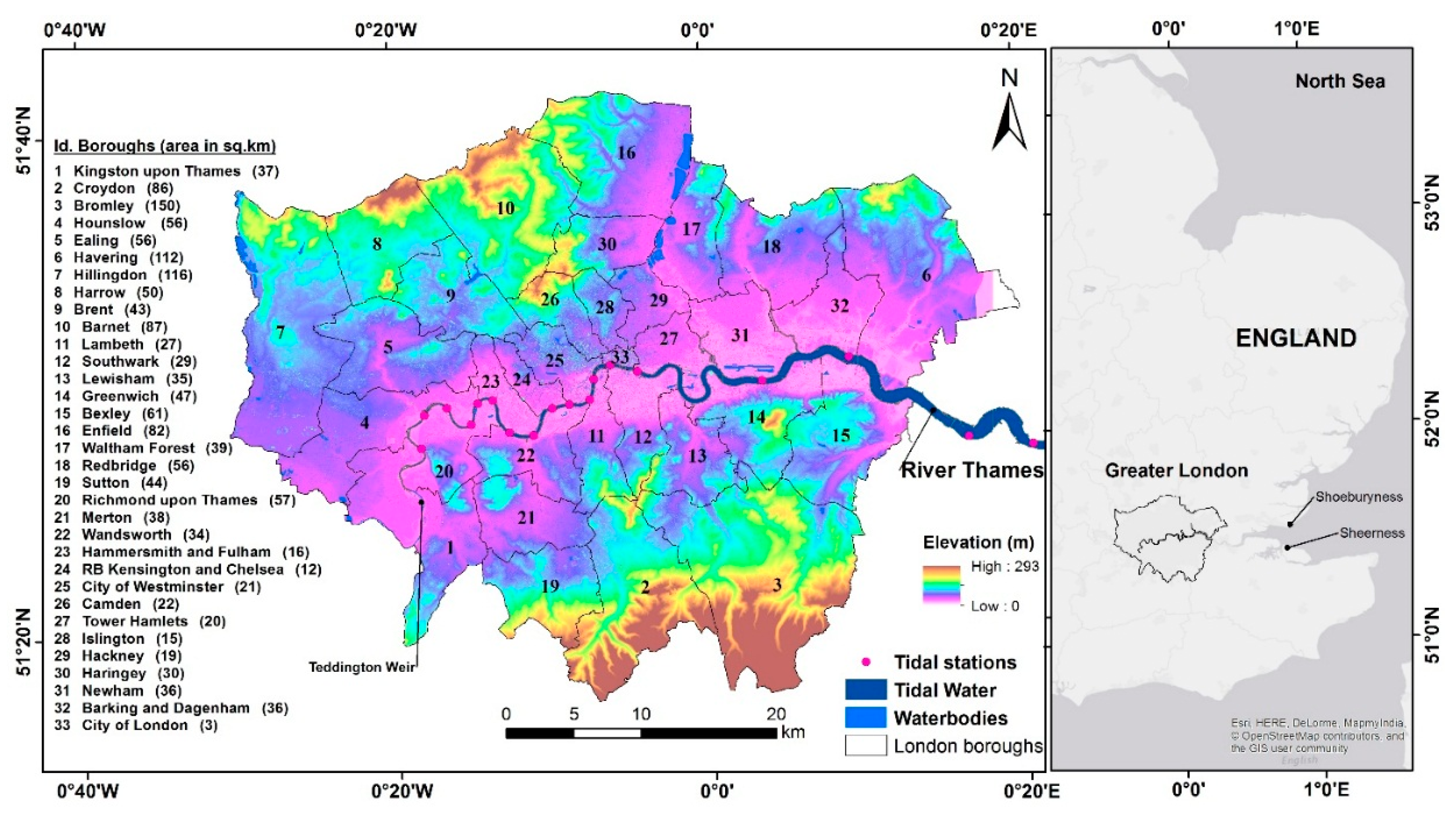
2.1. Elevation Data Sources
2.1.1. Ordnance Survey DEM
2.1.2. LiDAR DEM
2.1.3. SRTM DEM
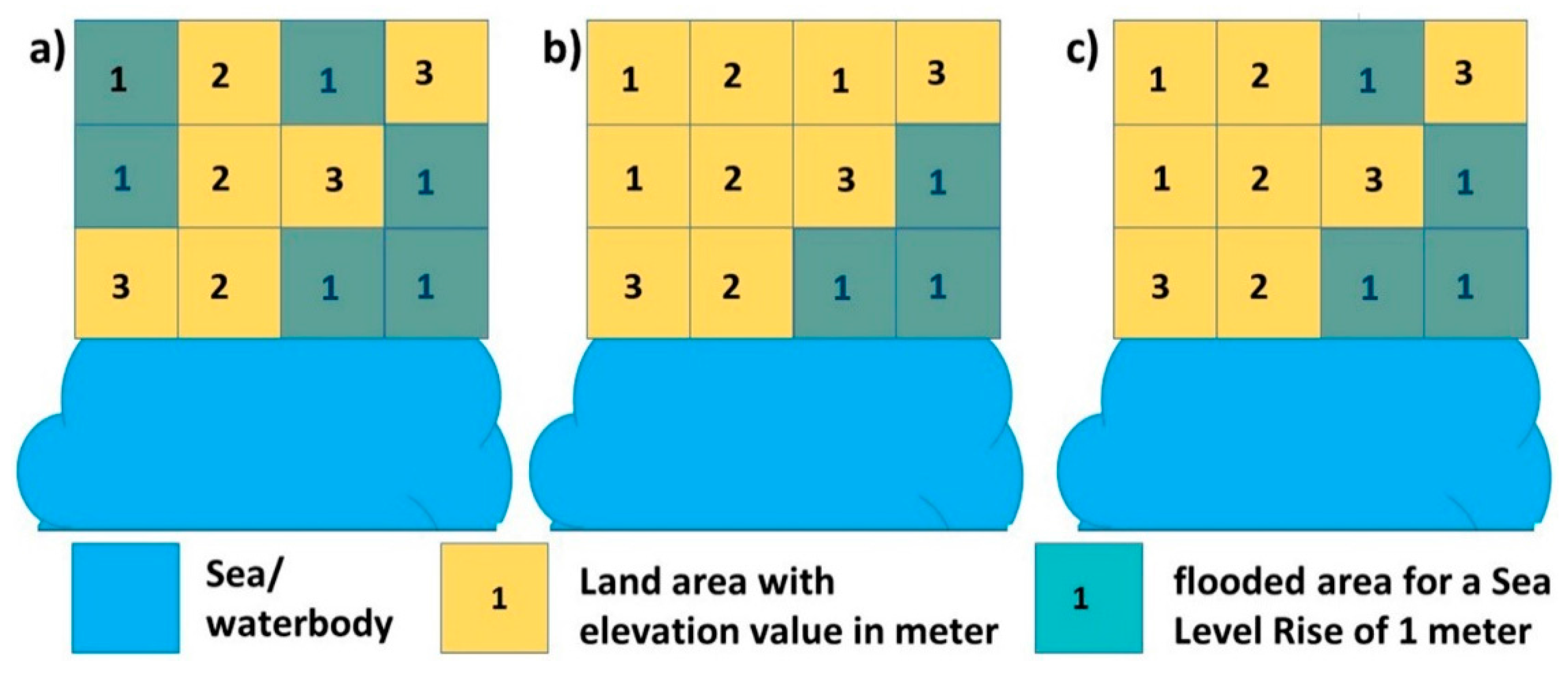
2.2. Inundation Model
2.3. Projected Sea Level Rise
2.3.1. Global
2.3.2. Regional
2.4. Tidal Surface Creation
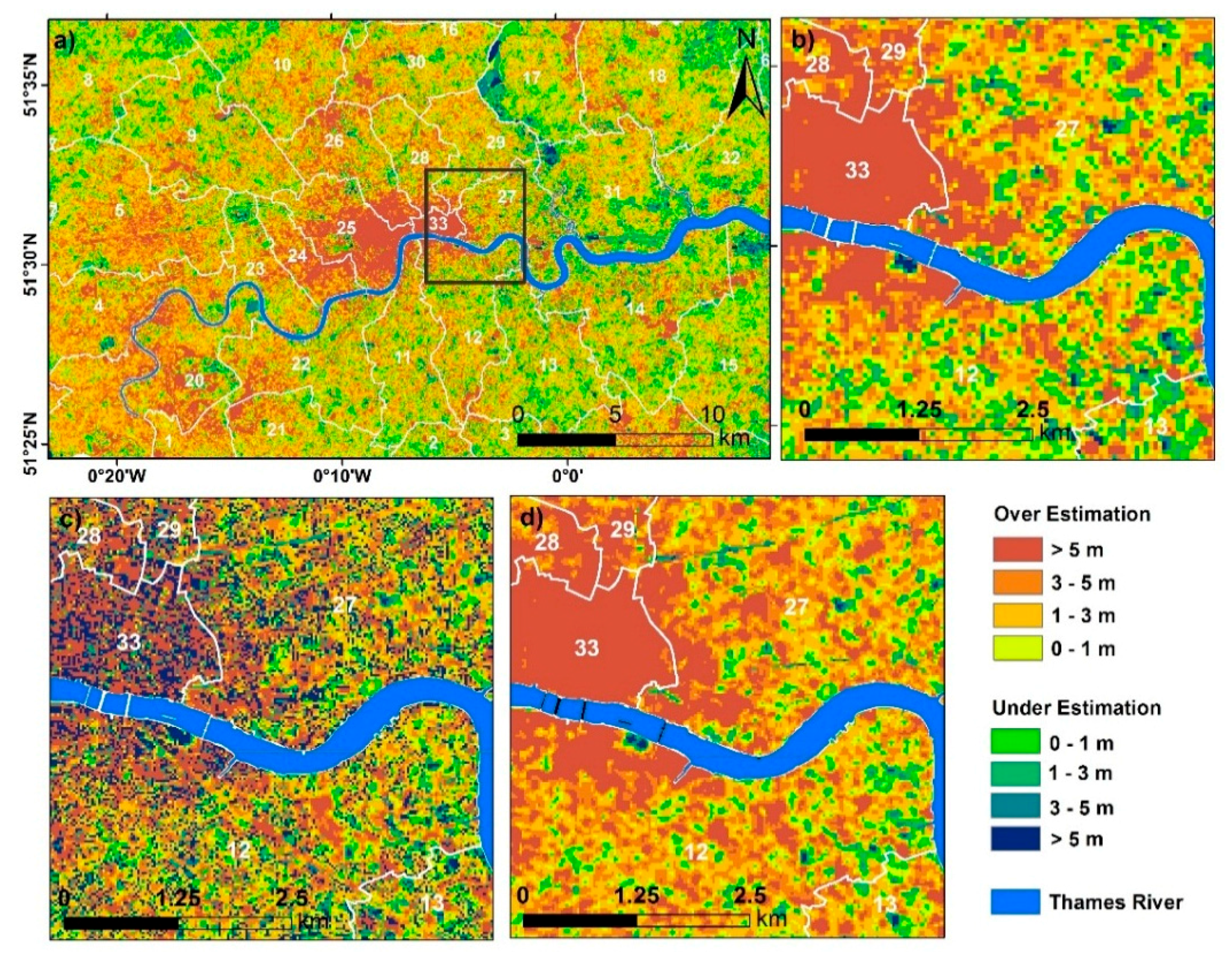
2.5. Accuracy Assessment
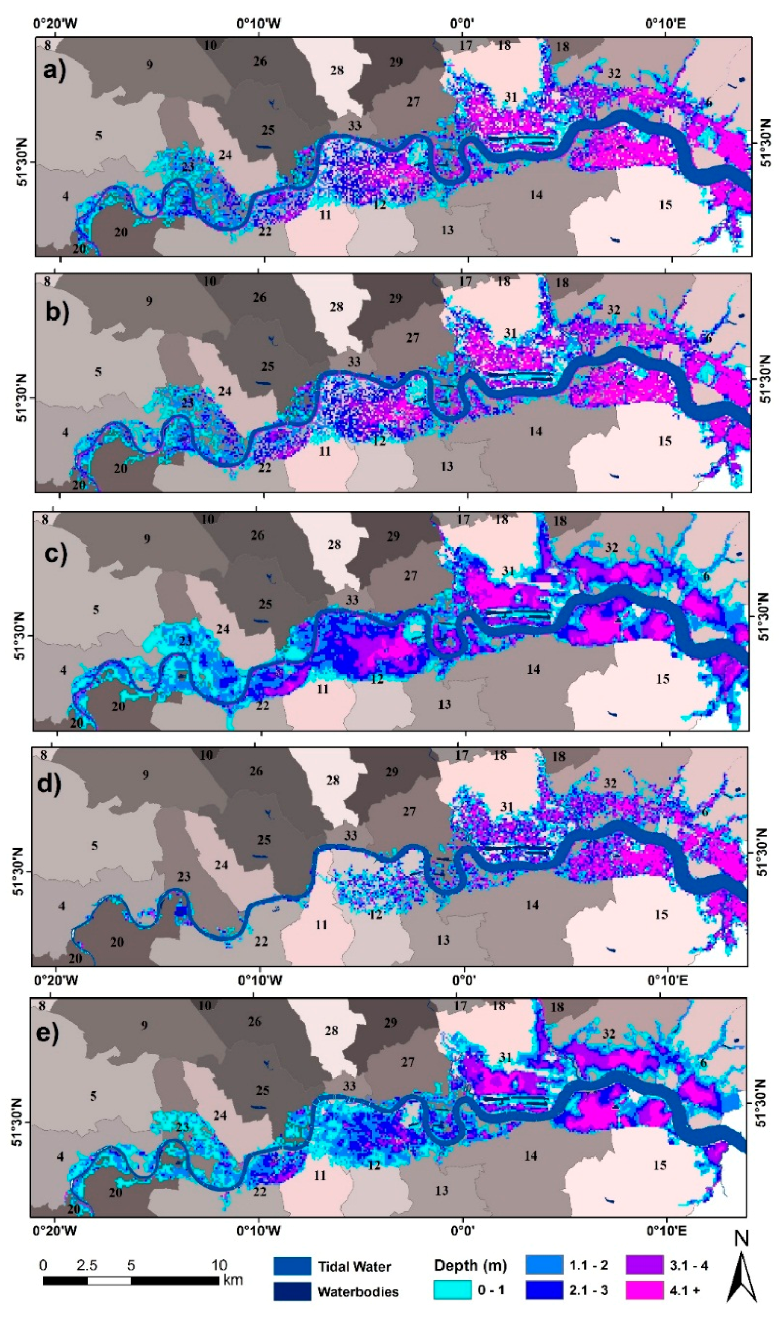
3. Results
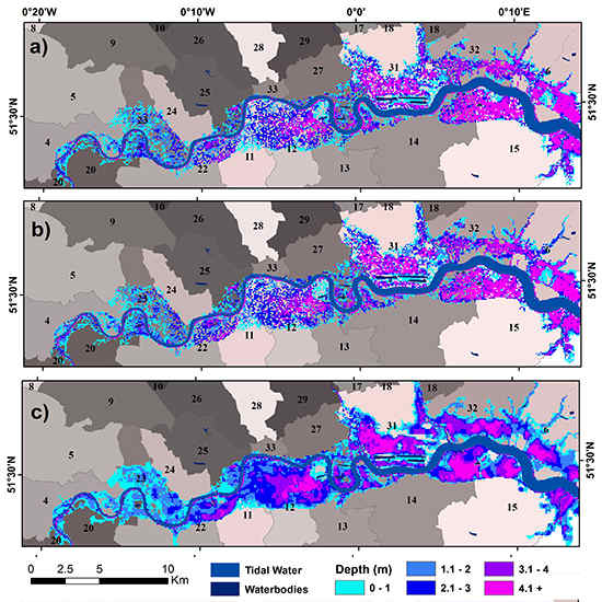
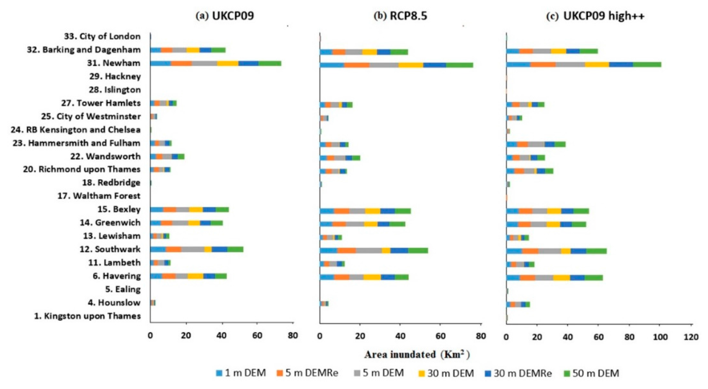
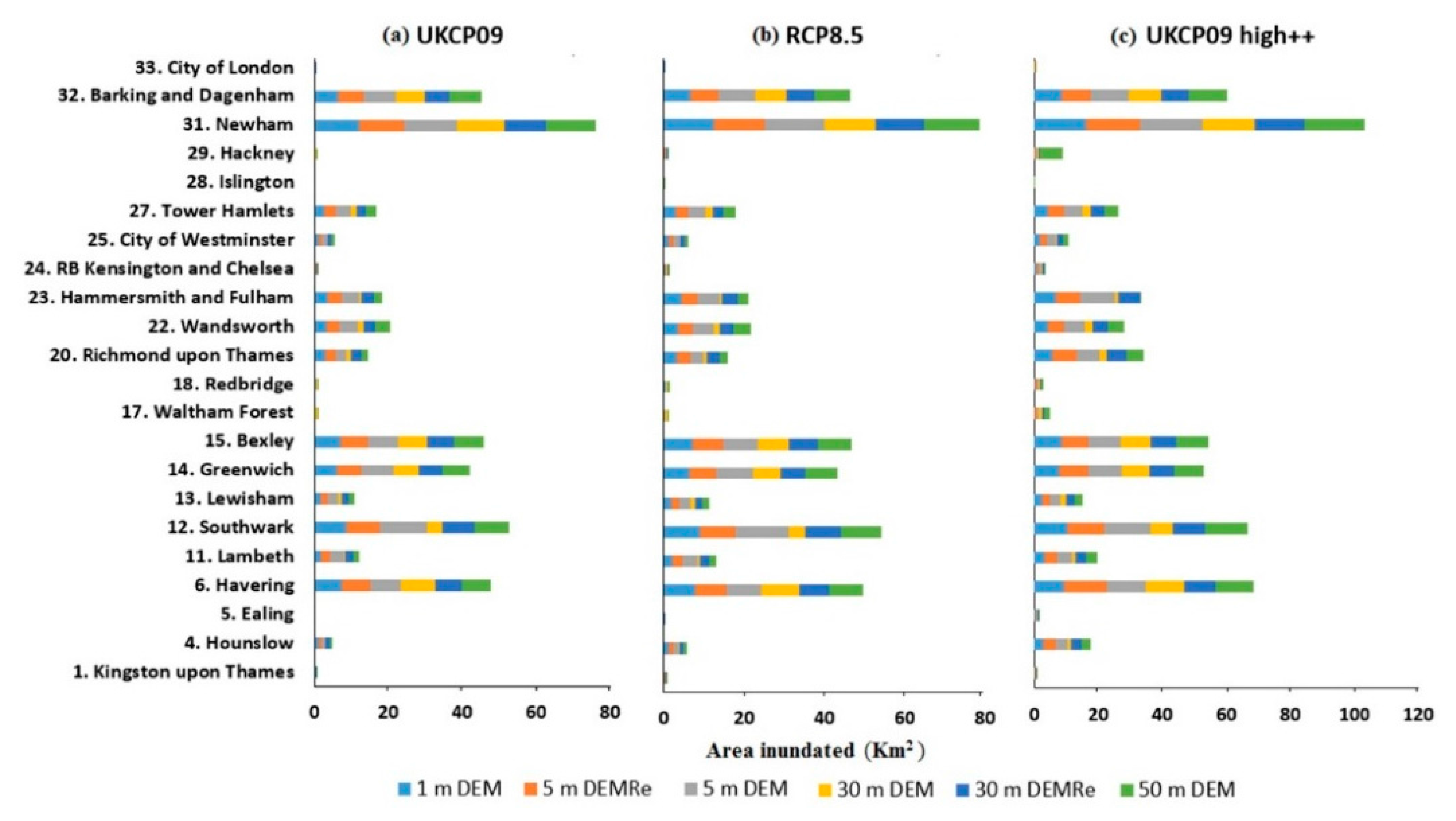
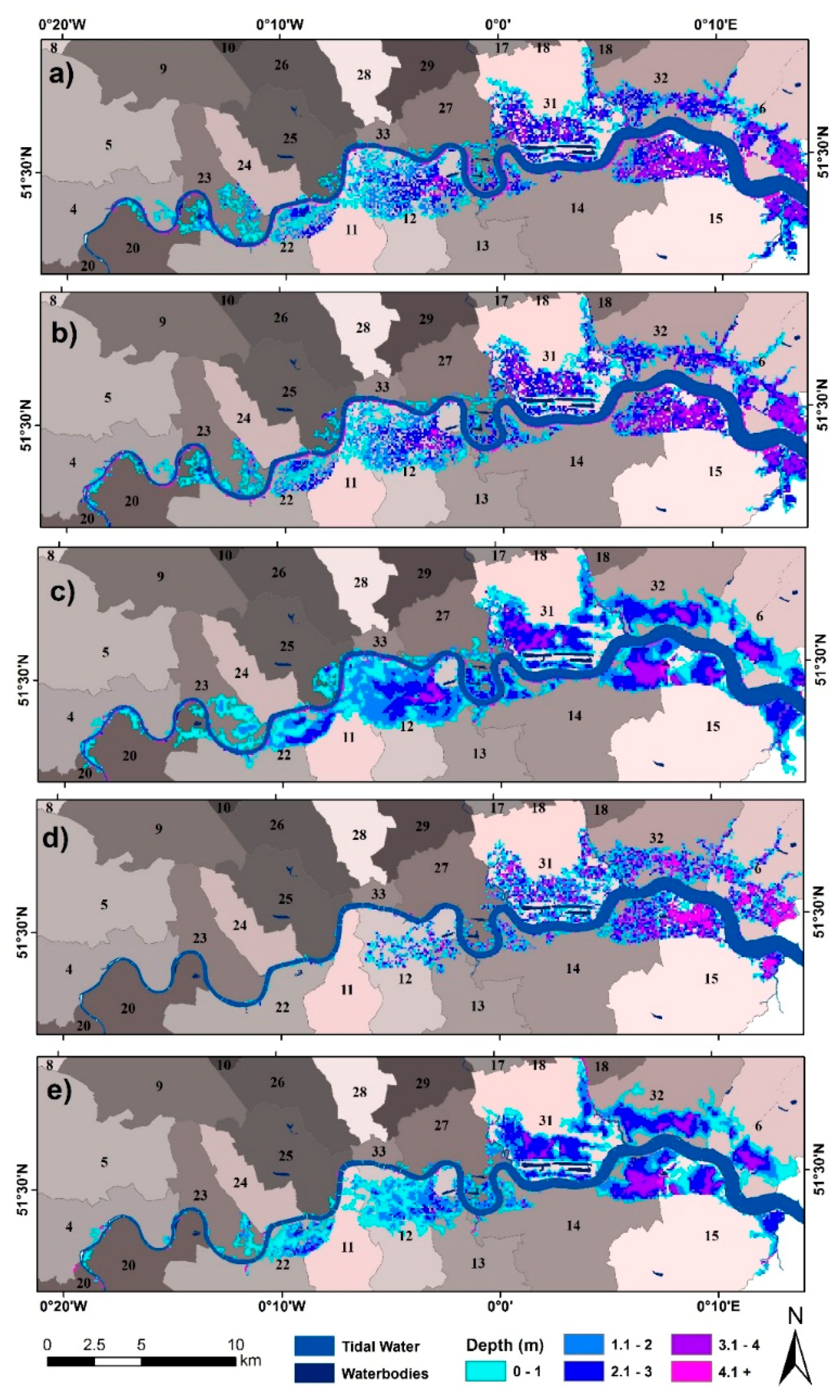
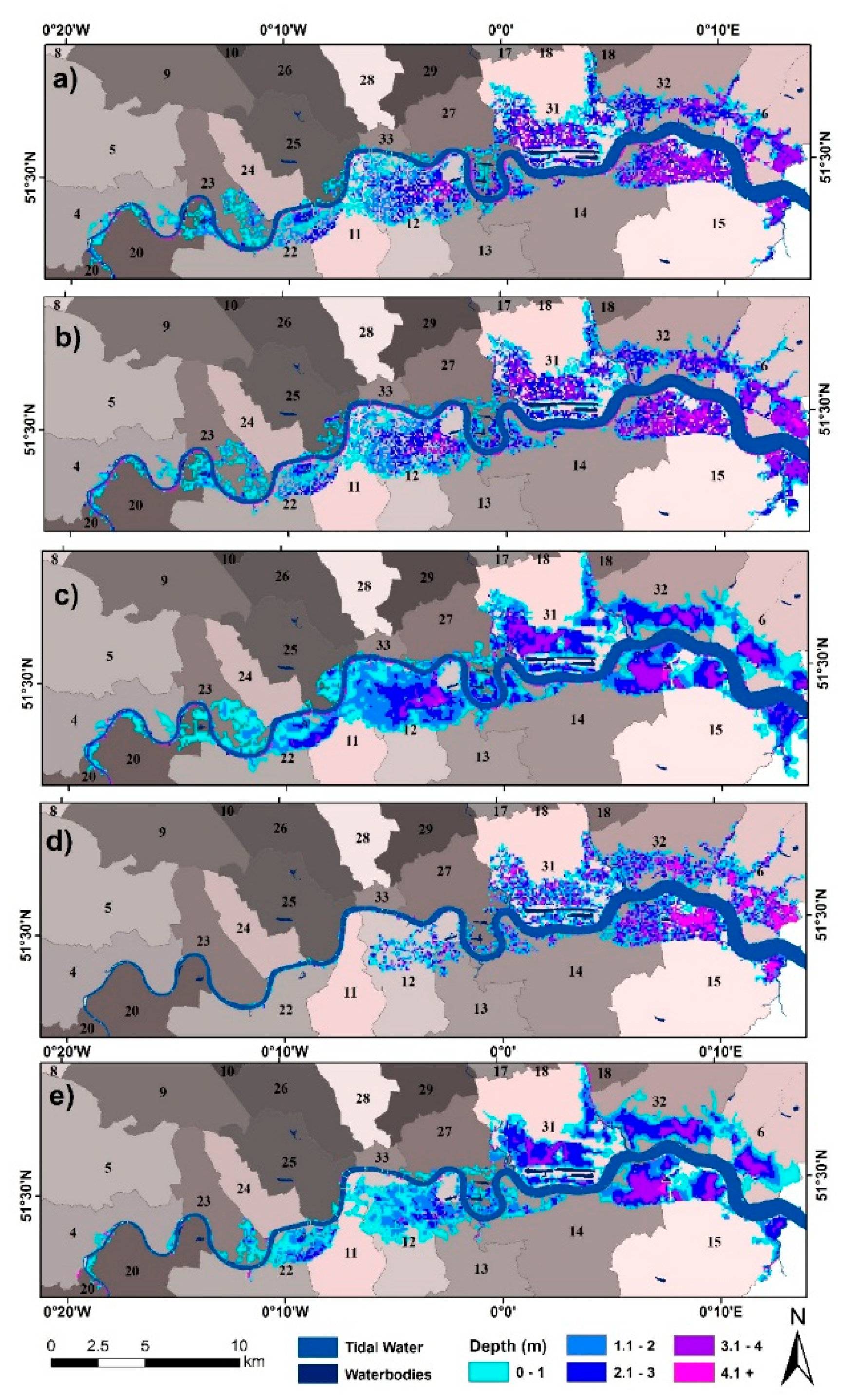
3.1. Scenario 1: 0.68 m SLR UKCP09
3.2. Scenario 2: 0.82 m SLR RCP8.5
3.3. Scenario 3: 1.90 m SLR UKCP09 High++
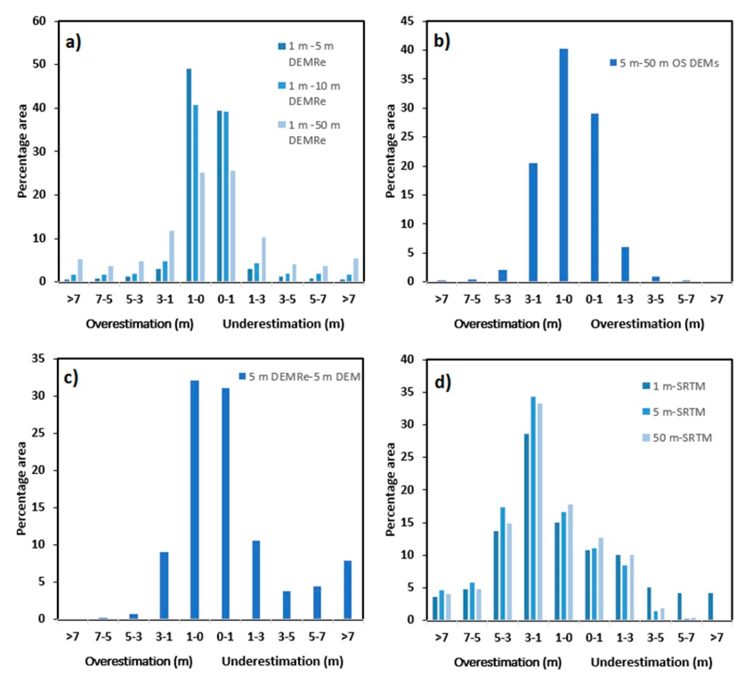
3.4. RMSE, NSSDA, and ME Estimation
4. Discussion
- (i)
- artefacts in the DEM resulting from the measurement source,
- (ii)
- artefacts introduced at the production stage,
- (iii)
- differences in processing methodology, and
- (iv)
- varying resolution of DEMs.
5. Conclusions
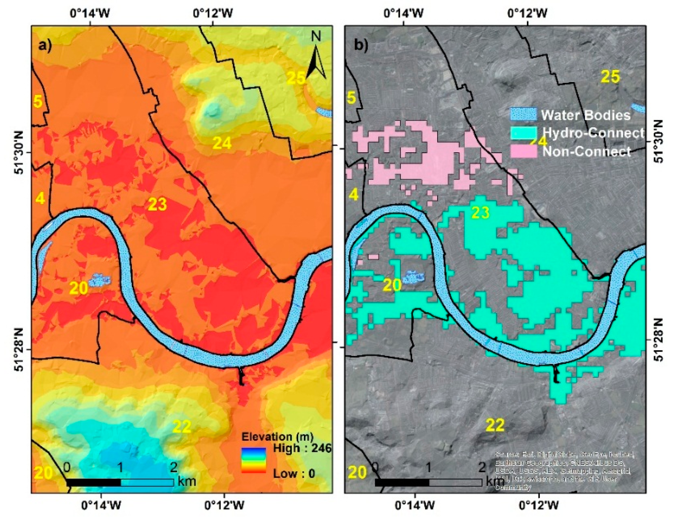
- (i)
- An eight-way connectivity bathtub approach gives significantly smaller flood inundation extents than the zero connectivity approach, indicating that the zero-connectivity approach may overestimate flooded areas due to the hydrological connectivity issue.
- (ii)
- Large variability in inundation estimates is observed for the same SLR scenario when using different elevation datasets, and this is attributed to differences in horizontal and vertical resolution, as well as processing methodologies.
- (iii)
- Flood inundation models developed using 1 m airborne LiDAR DEM give inundation extents between 61.76 and 91.77 km2 for three different SLR scenarios; 5 m DEMRe gives 64.24–96.60 km2; 5 m DEM gives 82.23–124.99 km2, 30 m DEMRe gives 61.64–91.04 km2, SRTM DEM gives 49.87–66.74 km2 and 50 m DEM gives 63.51–109.13 km2. Thus, while 1 m DEM, 5 m DEMRe, 30 m DEMRe, and 50 m DEM give similar inundation extents, the extents estimated by 5 m DEM are much larger, while the extents estimated by SRTM DEM are much smaller.
- (iv)
- Differences in inundation areas estimated between DSMs and DTMs for the same SLR scenarios are considerably larger than the RMSE differences between the datasets. As expected, using DTMs tends to result in higher inundation extents while using DSMs tends to result in lower inundation extents. Thus, we recommend to use a DTM and add objects using a DSM that may considerably influence the prediction such as large buildings, pillars of bridges, etc.
- (v)
- Flood inundation estimates using SRTM DEM appear to significantly underestimate inundation extents, possibly as a result of high RMSE and low vertical and horizontal resolution. Therefore, careful consideration should be made when assessing inundation zones from flood models using SRTM DEM.
- (vi)
- Although there are concerns about using DEMs having low spatial resolution, we recommend that the regionally available open data 50 m DEM be used for inundation studies of the UK rather than SRTM DEM, if no high-resolution data are available.
Acknowledgments
Author Contributions
Conflicts of Interest
Appendix

| Boroughs | 1 m DEM | 5 m DEMRe | 5 m DEM | 30 m DEM | 30 m DEMRe | 50 m DEM | ||||||
|---|---|---|---|---|---|---|---|---|---|---|---|---|
| 8-way | 0-connect | 8-way | 0-connect | 8-way | 0-connect | 8-way | 0-connect | 8-way | 0-connect | 8-way | 0-connect | |
| 1. Kingston upon Thames | - | 0.14 | - | 0.14 | - | - | - | 0.03 | - | 0.17 | - | 0.03 |
| 4. Hounslow | 0.59 | 1.08 | 0.69 | 1.01 | 0.45 | 0.91 | 0.17 | 0.24 | 0.72 | 1.10 | 0.38 | 0.78 |
| 5. Ealing | - | 0.02 | - | 0.02 | - | - | - | - | - | - | - | - |
| 6. Havering | 6.78 | 7.61 | 7.34 | 7.59 | 6.83 | 8.17 | 8.77 | 9.37 | 6.70 | 7.29 | 6.57 | 7.8 |
| 11. Lambeth | 1.94 | 1.96 | 2.21 | 2.24 | 3.74 | 3.79 | 0.03 | 0.44 | 2.14 | 2.16 | 1.29 | 1.42 |
| 12. Southwark | 8.76 | 8.82 | 8.67 | 8.88 | 12.91 | 12.92 | 4.1 | 4.09 | 8.62 | 8.70 | 9.09 | 9.34 |
| 13. Lewisham | 1.66 | 1.71 | 1.83 | 1.87 | 2.82 | 2.83 | 0.96 | 1.18 | 1.64 | 1.65 | 1.7 | 1.72 |
| 14. Greenwich | 6.13 | 6.36 | 6.3 | 6.4 | 8.89 | 8.91 | 6.66 | 6.84 | 5.82 | 6.03 | 7.04 | 7.66 |
| 15. Bexley | 7.19 | 7.28 | 7.34 | 7.43 | 7.38 | 8.06 | 7.56 | 7.96 | 7.06 | 7.18 | 7.64 | 7.9 |
| 17. Waltham Forest | 0.1 | 0.1 | 0.13 | 0.5 | 0.13 | 0.05 | ||||||
| 18. Redbridge | 0.08 | 0.2 | 0.10 | 0.12 | 0.08 | 0.3 | 0 | 0.18 | 0.12 | 0.15 | 0.35 | 0.35 |
| 20. Richmond upon Thames | 1.91 | 3.00 | 2.89 | 3.00 | 2.65 | 2.85 | 0.6 | 0.98 | 2.64 | 2.87 | 0.59 | 1.82 |
| 22. Wandsworth | 3.32 | 3.36 | 3.32 | 3.40 | 5.13 | 5.16 | 0.28 | 1.44 | 3.27 | 3.32 | 3.85 | 3.99 |
| 23. Hammersmith and Fulham | 2.64 | 3.74 | 2.1 | 3.79 | 3.41 | 4.61 | 0.09 | 0.5 | 2.39 | 3.56 | 1.34 | 2.11 |
| 24. RB Kensington and Chelsea | 0.14 | 0.27 | 0.12 | 0.21 | 0.11 | 0.2 | 0.02 | 0.06 | 0.16 | 0.26 | 0.03 | 0.06 |
| 25. City of Westminster | 0.54 | 1.06 | 0.85 | 1.05 | 1.47 | 1.5 | 0.06 | 0.1 | 0.62 | 1.05 | 0.18 | 0.8 |
| 27. Tower Hamlets | 2.44 | 2.83 | 2.71 | 2.98 | 3.94 | 4.02 | 1.23 | 1.7 | 2.33 | 2.56 | 2.28 | 2.79 |
| 28. Islington | 0.01 | 0.01 | 0.01 | - | 0.01 | |||||||
| 29. Hackney | - | 0.08 | - | 0.14 | - | 0.2 | - | 0.19 | - | 0.08 | 0.08 | |
| 31. Newham | 11.55 | 12.00 | 11.76 | 12.23 | 14.29 | 14.58 | 11.99 | 12.58 | 11.00 | 11.54 | 12.88 | 13.28 |
| 32. Barking and Dagenham | 6.05 | 6.54 | 6.23 | 6.73 | 8.07 | 8.73 | 7.34 | 7.97 | 6.40 | 6.60 | 8.29 | 8.6 |
| 33. City of London | 0.05 | 0.05 | 0.02 | 0.02 | 0.06 | 0.06 | 0.01 | 0.01 | ||||
| Total | 61.76 | 68.24 | 64.49 | 69.37 | 82.23 | 87.95 | 49.87 | 56.36 | 61.64 | 66.41 | 63.51 | 70.6 |
| Boroughs | 1 m DEM | 5 m DEMRe | 5 m DEM | 30 m DEM | 30 m DEMRe | 50 m DEM | ||||||
|---|---|---|---|---|---|---|---|---|---|---|---|---|
| 8-way | 0-connect | 8-way | 0-connect | 8-way | 0-connect | 8-way | 0-connect | 8-way | 0-connect | 8-way | 0-connect | |
| 1. Kingston upon Thames | 0.15 | 0.14 | 0.01 | 0.03 | 0.17 | 0.03 | ||||||
| 4. Hounslow | 1.05 | 1.25 | 0.87 | 1.12 | 0.89 | 1.17 | 0.17 | 0.24 | 0.94 | 1.28 | 0.5 | 0.91 |
| 5. Ealing | 0.04 | 0.04 | 0.04 | |||||||||
| 6. Havering | 7 | 7.9 | 7.45 | 7.72 | 7.23 | 8.68 | 8.77 | 9.37 | 6.90 | 7.56 | 6.9 | 8.26 |
| 11. Lambeth | 2.16 | 2.16 | 2.35 | 2.38 | 3.95 | 3.96 | 0.03 | 0.44 | 2.37 | 2.38 | 1.53 | 1.67 |
| 12. Southwark | 8.91 | 8.96 | 8.96 | 9.05 | 13.11 | 13.12 | 4.1 | 4.09 | 8.78 | 8.87 | 9.98 | 10.23 |
| 13. Lewisham | 1.7 | 1.75 | 1.94 | 1.98 | 2.87 | 2.87 | 0.96 | 1.18 | 1.71 | 1.73 | 1.86 | 1.87 |
| 14. Greenwich | 6.28 | 6.52 | 6.52 | 6.57 | 9.13 | 9.15 | 6.66 | 6.84 | 6.01 | 6.24 | 7.8 | 7.88 |
| 15. Bexley | 7.26 | 7.37 | 7.4 | 7.49 | 7.95 | 8.41 | 7.56 | 7.96 | 7.13 | 7.26 | 7.94 | 8.13 |
| 17. Waltham Forest | 0.1 | 0.1 | 0.14 | 0.5 | 0.14 | 0.05 | ||||||
| 18. Redbridge | 0.08 | 0.22 | 0.12 | 0.15 | 0.31 | 0.31 | 0.18 | 0.14 | 0.18 | 0.36 | 0.36 | |
| 20. Richmond upon Thames | 2.96 | 3.27 | 3.17 | 3.29 | 3.07 | 3.26 | 0.6 | 0.98 | 2.88 | 3.06 | 0.71 | 2.1 |
| 22. Wandsworth | 3.5 | 3.56 | 3.5 | 3.58 | 5.39 | 5.39 | 0.28 | 1.44 | 3.39 | 3.47 | 3.97 | 4.13 |
| 23. Hammersmith and Fulham | 2.94 | 4.28 | 2.84 | 4.2 | 3.95 | 5.54 | 0.09 | 0.5 | 2.78 | 4.10 | 1.62 | 2.52 |
| 24. RB Kensington and Chelsea | 0.15 | 0.32 | 0.14 | 0.23 | 0.13 | 0.23 | 0.02 | 0.06 | 0.17 | 0.31 | 0.03 | 0.08 |
| 25. City of Westminster | 0.62 | 1.16 | 1.06 | 1.17 | 1.72 | 1.72 | 0.06 | 0.1 | 0.66 | 1.10 | 0.21 | 0.95 |
| 27. Tower Hamlets | 2.69 | 3 | 2.84 | 3.13 | 4.18 | 4.24 | 1.23 | 1.7 | 2.51 | 2.74 | 2.9 | 3.02 |
| 28. Islington | 0.02 | 0.01 | 0.01 | 0.01 | ||||||||
| 29. Hackney | 0.12 | 0.16 | 0.23 | 0.19 | 0.09 | 0.08 | ||||||
| 31. Newham | 11.96 | 12.42 | 12.43 | 12.68 | 14.87 | 15.11 | 11.99 | 12.58 | 11.49 | 11.97 | 13.33 | 13.86 |
| 32. Barking and Dagenham | 6.26 | 6.77 | 6.48 | 6.96 | 8.45 | 9.03 | 7.34 | 7.97 | 6.55 | 6.80 | 8.69 | 8.98 |
| 33. City of London | 0.06 | 0.06 | 0.03 | 0.03 | 0.06 | 0.06 | 0.02 | 0.02 | ||||
| Total | 65.57 | 71.42 | 68.09 | 72.18 | 87.26 | 92.64 | 49.87 | 56.36 | 64.43 | 69.51 | 68.34 | 75.11 |
| Boroughs | 1 m DEM | 5 m DEMRe | 5 m DEM | 30 m DEM | 30 m DEMRe | 50 m DEM | ||||||
|---|---|---|---|---|---|---|---|---|---|---|---|---|
| 8-way | 0-connect | 8-way | 0-connect | 8-way | 0-connect | 8-way | 0-connect | 8-way | 0-connect | 8-way | 0-connect | |
| 1. Kingston upon Thames | 0.18 | 0.22 | 0.05 | 0.06 | 0.60 | 0.20 | 0.01 | 0.08 | ||||
| 4. Hounslow | 2.8 | 2.73 | 2.91 | 3.91 | 3.82 | 3.85 | 0.06 | 0.93 | 2.95 | 3.24 | 2.89 | 2.96 |
| 5. Ealing | 0.22 | 0.24 | 0.24 | 0.38 | 0.31 | 0.31 | 0 | 0.01 | 0.27 | 0.27 | 0.01 | 0.03 |
| 6. Havering | 8.89 | 9.48 | 9.7 | 13.15 | 12.16 | 12.21 | 10.76 | 12.03 | 9.49 | 9.74 | 11.79 | 12.08 |
| 11. Lambeth | 3.07 | 3.22 | 3.22 | 3.76 | 4.92 | 4.92 | 0.3 | 0.9 | 3.18 | 3.24 | 3.67 | 3.72 |
| 12. Southwark | 10.37 | 10.51 | 10.51 | 11.34 | 14.63 | 14.64 | 6.24 | 6.65 | 10.31 | 10.32 | 13.39 | 13.39 |
| 13. Lewisham | 2.27 | 2.36 | 2.48 | 2.58 | 3.28 | 3.36 | 1.69 | 1.85 | 2.24 | 2.32 | 2.74 | 2.78 |
| 14. Greenwich | 7.84 | 8 | 8.05 | 8.72 | 10.54 | 10.61 | 8.5 | 8.55 | 7.65 | 7.75 | 9.5 | 9.57 |
| 15. Bexley | 8.2 | 8.47 | 8.51 | 8.59 | 10 | 10.1 | 9.11 | 9.18 | 7.98 | 8.18 | 9.78 | 9.94 |
| 17. Waltham Forest | 0.5 | 0.69 | 0.66 | 1.14 | 0.52 | 2.04 | ||||||
| 18. Redbridge | 0.47 | 0.4 | 0.43 | 0.5 | 0.56 | 0.56 | 0.02 | 0.37 | 0.38 | 0.39 | 0.54 | 0.54 |
| 20. Richmond upon Thames | 5.48 | 5.66 | 5.88 | 7.69 | 6.92 | 7.09 | 1.42 | 2.31 | 5.56 | 5.95 | 5.38 | 5.51 |
| 22. Wandsworth | 4.24 | 4.31 | 4.49 | 5.02 | 6.46 | 6.46 | 0.68 | 2.57 | 4.33 | 4.51 | 5.09 | 5.15 |
| 23. Hammersmith and Fulham | 7.14 | 6.78 | 6.92 | 7.57 | 10.52 | 10.69 | 0.39 | 1.36 | 6.29 | 6.68 | 7.23 | 0.11 |
| 24. RB Kensington and Chelsea | 0.63 | 0.5 | 0.67 | 0.92 | 0.78 | 0.82 | 0.03 | 0.1 | 0.71 | 0.33 | 0.34 | |
| 25. City of Westminster | 1.73 | 1.84 | 1.89 | 2.06 | 2.94 | 2.94 | 0.07 | 0.16 | 1.79 | 1.83 | 2.01 | 2.04 |
| 27. Tower Hamlets | 4.05 | 4.39 | 4.49 | 4.76 | 5.81 | 5.93 | 2.17 | 2.71 | 4.00 | 4.13 | 4.42 | 4.52 |
| 28. Islington | 0.01 | 0.01 | 0.01 | |||||||||
| 29. Hackney | 0.37 | 0.4 | 0.08 | 0.58 | 0.31 | 0.28 | 7.23 | |||||
| 31. Newham | 15.76 | 16.02 | 16.31 | 17.22 | 19.3 | 19.37 | 15.36 | 16.22 | 15.51 | 15.78 | 18.39 | 18.63 |
| 32. Barking and Dagenham | 8.53 | 8.51 | 8.81 | 9.07 | 11.81 | 11.83 | 9.93 | 10.38 | 8.45 | 8.70 | 11.92 | 11.92 |
| 33. City of London | 0.09 | 0.04 | 0.05 | 0.06 | 0.17 | 0.17 | 0.06 | 0.06 | 0.05 | 0.05 | ||
| Total | 91.77 | 93.45 | 96.6 | 108.61 | 124.99 | 127.14 | 66.74 | 77.78 | 91.04 | 94.76 | 109.13 | 112.65 |
References
- Church, J.A.; Clark, P.U.; Cazenave, A.; Gregory, J.M.; Jevrejeva, S.; Levermann, A.; Merrifield, M.A.; Milne, G.A.; Nerem, R.S.; Nunn, P.D.; et al. Sea level change. In Climate Change 2013: The Physical Science Basis. Contribution of Working Group I to the Fifth Assessment Report of the Intergovernmental Panel on Climate Change; PM Cambridge University Press: Cambridge, UK; New York, NY, USA, 2013; pp. 1137–1216. [Google Scholar]
- Hirabayashi, Y.; Mahendran, R.; Koirala, S.; Konoshima, L.; Yamazaki, D.; Watanabe, S.; Kim, H.; Kanae, S. Global flood risk under climate change. Nat. Climate Chang. 2013, 3, 816–821. [Google Scholar] [CrossRef]
- Rowley, R.J.; Kostelnick, J.C.; Braaten, D.; Li, X.; Meisel, J. Risk of rising sea level to population and land area. Eos, Trans. Am. Geophys. Union 2007, 88, 105–116. [Google Scholar] [CrossRef]
- Mcleod, E.; Poulter, B.; Hinkel, J.; Reyes, E.; Salm, R. Sea-Level rise impact models and environmental conservation: A review of models and their applications. Ocean Coast. Manag. 2010, 53, 507–517. [Google Scholar] [CrossRef]
- Chen, J.; Hill, A.A.; Urbano, L.D. A GIS-based model for urban flood inundation. J. Hydrol. 2009, 373, 184–192. [Google Scholar] [CrossRef]
- Gesch, D.B. Consideration of vertical uncertainty in elevation-based sea-level rise assessments: Mobile Bay, Alabama case study. J. Coast. Res. 2013, 63, 197–210. [Google Scholar] [CrossRef]
- Gesch, D.B. Analysis of LiDAR elevation data for improved identification and delineation of lands vulnerable to sea-level rise. J. Coast. Res. 2009, 10053, 49–58. [Google Scholar] [CrossRef]
- Li, J.; Wong, D.W. Effects of DEM sources on hydrologic applications. Comput. Environ. Urban Syst. 2010, 34, 251–261. [Google Scholar]
- Tsanis, I.; Seiradakis, K.; Daliakopoulos, I.; Grillakis, M.; Koutroulis, A. Assessment of GeoEye-1 stereo-pair-generated DEM in flood mapping of an ungauged basin. J. Hydroinf. 2014, 16, 1–18. [Google Scholar] [CrossRef]
- Langridge, R.; Ries, W.; Farrier, T.; Barth, N.; Khajavi, N.; De Pascale, G. Developing Sub 5-m LiDAR DEMs for forested sections of the alpine and hope faults, South Island, New Zealand: Implications for structural interpretations. J. Struct. Geol. 2014, 64, 53–66. [Google Scholar] [CrossRef]
- Hayakawa, Y.S.; Oguchi, T.; Saito, H.; Kobayashi, A.; Baker, V.R.; Pelletier, J.D.; McGuire, L.A.; Komatsu, G.; Goto, K. Geomorphic imprints of repeated tsunami waves in a coastal valley in northeastern Japan. Geomorphology 2015, 242, 3–10. [Google Scholar] [CrossRef]
- Jiang, H.; Zhang, L.; Wang, Y.; Liao, M. Fusion of high-resolution DEMs derived from COSMO-SkyMed and TerraSAR-X InSAR datasets. J. Geodesy 2014, 88, 587–599. [Google Scholar] [CrossRef]
- Mancini, F.; Dubbini, M.; Gattelli, M.; Stecchi, F.; Fabbri, S.; Gabbianelli, G. Using unmanned aerial vehicles (UAV) for high-resolution reconstruction of topography: The Structure from motion approach on coastal environments. Remote Sens. 2013, 5, 6880–6898. [Google Scholar] [CrossRef] [Green Version]
- Gomez, C.; Hayakawa, Y.; Obanawa, H. A Study of Japanese landscapes using structure from motion derived DSMs and DEMs based on historical aerial photographs: New opportunities for vegetation monitoring and diachronic geomorphology. Geomorphology 2015, 242, 11–20. [Google Scholar] [CrossRef]
- Mukherjee, S.; Joshi, P.K.; Mukherjee, S.; Ghosh, A.; Garg, R.D.; Mukhopadhyay, A. Evaluation of vertical accuracy of open source digital elevation model (DEM). Int. J. Appl. Earth Obs. Geoinform. 2012, 21, 205–217. [Google Scholar] [CrossRef]
- Rodriguez, E.; Morris, C.S.; Belz, J.E. A Global assessment of the SRTM performance. Photogramm. Eng. Remote Sens. 2006, 72, 249–260. [Google Scholar] [CrossRef]
- Polidori, L.; Chorowicz, J.; Guillande, R. Description of terrain as a fractal surface, and application to digital elevation model quality assessment. Photogramm. Eng. Remote Sens. 1991, 57, 1329–1332. [Google Scholar]
- Carter, J.R. The effect of data precision on the calculation of slope and aspect using gridded DEMs. Cartographica 1992, 29, 22–34. [Google Scholar] [CrossRef]
- Triglav-Čekada, M.; Crosilla, F.; Kosmatin-Fras, M. A simplified analytical model for a-priori LiDAR point-positioning error estimation and a review of LiDAR error sources. Photogramm. Eng. Remote Sens. 2009, 75, 1425–1439. [Google Scholar] [CrossRef]
- Cooper, M.A.R. Datums, coordinates and differences. In Landform Monitoring, Modelling and Analysis; Wiley: Chichester, UK, 1998; pp. 21–36. [Google Scholar]
- Hunter, G.J.; Goodchild, M.F. Mapping uncertainty in spatial databases, putting theory into practice. J. Urban Reg. Inf. Syst. Assoc. 1993, 5, 55–62. [Google Scholar]
- Kraus, K. Visualization of the quality of surfaces and their derivatives. Photogramm. Eng. Remote Sens. 1994, 60, 457–462. [Google Scholar]
- Fisher, P.F.; Tate, N.J. Causes and consequences of error in digital elevation models. Prog. Phys. Geogr. 2006, 30, 467–489. [Google Scholar] [CrossRef]
- Leon, J.X.; Heuvelink, G.B.M.; Phinn, S.R. Incorporating DEM uncertainty in coastal inundation mapping. PLoS ONE 2014, 9, e108727. [Google Scholar] [CrossRef] [PubMed]
- Shearer, J.W. The accuracy of digital terrain models. In Terrain Modelling in Surveying and Civil Engineering; Petrie, G., Kennie, T.J.M., Eds.; Caithness, Whittles Publishing: New York, NY, USA, 1990; pp. 315–336. [Google Scholar]
- Greater London Authority. Flooding. Available online: https://www.london.gov.uk/mayor-assembly/mayor/london-resilience/risks/flooding (accessed on 16 September 2015).
- Environmental Agency. TE2100 Plan. Managing Flood Risk Through London and the Thames Estuary; Environmental Agency: London, UK, 2012.
- Lavery, S.; Donovan, B. Flood risk management in the Thames estuary looking ahead 100 years. Philos. Trans. Ser. A 2005, 363, 1455–1474. [Google Scholar] [CrossRef] [PubMed]
- Greater London Authority. London Resilience, London Strategic Flood Framework Version 2. Available online: https://www.london.gov.uk/sites/default/files/London-Strategic-Flood-Framework-V2_1.pdf (accessed on 12 April 2012).
- Guardian. Beyond the Thames Barrier: How Safe is London from Another Major Flood? Available online: http://www.theguardian.com/cities/2015/feb/19/thames-barrier-how-safe-london-major-flood-at-risk (accessed on 13 August 2015).
- Marsh, T.J. The Risk of Tidal Flooding in London. Climate, Hydrology, Sea Level and Air Pollution. Available online: http://www.ecn.ac.uk/iccuk/indicators/10.htm (accessed on 13 August 2015).
- Dawson, R.J.; Hall, J.W.; Bates, P.D.; Nicholls, R.J. Quantified analysis of the probability of flooding in the Thames estuary under imaginable worst case sea-level rise scenarios. Int. J. Water Res. Dev. 2005. [Google Scholar] [CrossRef]
- Aeromatrex. Digital Elevation, Digital Terrain or Digital Surface Model? Available online: http://www.aeromatrex.co,.au/blog/?p=89 (accessed on 20 February 2016).
- OS Terrain 50 DTM. Available online: http://www.Ordnancesurvey.Co.uk/opendata/ (accessed on 13 February 2015).
- OS Terrain 5 DTM. [ASC Geospatial Data], Scale 1:10,000, Updated: 23 September 2014, Ordnance Survey (GB), Using: EDINA Digimap Ordnance Survey Service. Available online: http://digimap.edina.ac.uk (accessed on 2 February 2015).
- Lindberg, F.; Grimmond, C.S.B.; Martilli, A. Sunlit fractions on urban facets—Impact of spatial resolution and approach. Urban Clim. 2015, 12, 65–84. [Google Scholar] [CrossRef]
- Shi, W.; Wang, B.; Tian, Y. Accuracy analysis of digital elevation model relating to spatial resolution and terrain slope by bilinear interpolation. Math. Geosci. 2014, 46, 445–481. [Google Scholar] [CrossRef]
- Lin, S.; Jing, C.; Coles, N.A.; Chaplot, V.; Moore, N.J.; Wu, J. Evaluating DEM source and resolution uncertainties in the soil and water assessment tool. Stoch. Environ. Res. Risk Assess. 2013, 27, 209–221. [Google Scholar] [CrossRef]
- Zhou, Y.; Chen, J.; Guo, Q.; Cao, R.; Zhu, X. Restoration of information obscured by mountainous shadows through Landsat TM/ETM images without the use of DEM data: A new method. IEEE Trans. Geosci. Remote Sens. 2014, 52, 313–328. [Google Scholar] [CrossRef]
- USGS. Shuttle Radar Topography Mission (SRTM) 1 Arc-Second Global. Available online: https://lta.Cr.Usgs.gov/SRTM1Arc (accessed on 16 September 2015).
- JPL/NASA. U.S. Releases Enhanced Shuttle Land Elevation Data. Available online: http://www2.Jpl.Nasa.gov/srtm/ (accessed on 16 September 2015).
- Vaan de Sante, B.; Lansen, J.; Claartje, H. Sensitivity of coastal flood risk assessments to digital elevation models. Water 2012, 4, 568–579. [Google Scholar] [CrossRef]
- Titus, J.G.; Richman, C. Maps of lands vulnerable to sea level rise: Modeled elevations along the US Atlantic and Gulf Coasts. Clim. Res. 2001, 18, 205–228. [Google Scholar] [CrossRef]
- Strauss, B.H.; Ziemlinski, R.; Weiss, J.L.; Overpeck, J.T. Tidally adjusted estimates of topographic vulnerability to sea level rise and flooding for the contiguous United States. Environ. Res. Lett. 2012, 7, 014033. [Google Scholar] [CrossRef]
- Poulter, B.; Halpin, P.N. Raster modelling of coastal flooding from sea-level rise. Int. J. Geogr. Inf. Sci. 2008, 22, 167–182. [Google Scholar] [CrossRef]
- Gallien, T.W.; Sanders, B.F.; Flick, R.E. Urban coastal flood prediction: integrating wave overtopping, flood defences and drainage. Coast. Eng. 2014, 91, 18–28. [Google Scholar] [CrossRef]
- Seenath, A.; Wilson, M.; Miller, K. Hydrodynamic versus GIS modelling for coastal flood vulnerability assessment: Which is better for guiding coastal management. Ocean Coast. Manag. 2016, 120, 99–109. [Google Scholar] [CrossRef]
- Wong, P.P.; Losada, I.J.; Gattuso, J.P.; Hinkel, J.; Khattabi, A.; McInnes, K.L.; Saito, Y.; Sallenger, A. Coastal Systems and Low-Lying Areas. in: Climate Change 2014: Impacts, Adaptation, and Vulnerability. Part A: Global and Sectoral Aspects. Contribution of Working Group II to the Fifth Assessment Report of the Intergovernmental Panel on Climate Change; Field, C.B., Barros, V.R., Dokken, D.J., Mach, K.J., Mastrandrea, M.D., Bilir, T.E., Chatterjee, M., Ebi, K.L., Estrada, Y.O., Genova, R.C., et al., Eds.; Cambridge University Press: Cambridge, UK; New York, NY, USA, 2014; pp. 361–409. [Google Scholar]
- Wong, P. Impacts and recovery from a large tsunami: Coasts of Aceh. Pol. J. Environ. Stud. 2009, 18, 5–16. [Google Scholar]
- IPCC. Contribution of Working Groups I, II and III to the Fourth Assessment Report of the Intergovernmental panel on climate change. In Climate change 2007: Synthesis Report; IPCC: Genewa, Switzerland, 2007. [Google Scholar]
- Defra. Adapting to climate change UK climate projections. UK Clim. Proj. 2009, 52, 1–42. [Google Scholar]
- Lowe, J.; Howard, T.; Pardaens, A.; Tinker, J.; Holt, J.; Wakelin, S.; Milne, G.; Leake, J.; Wolf, J.; Horsburgh, K. UK Climate Projections Science Report: Marine and Coastal Projections; Met Office Hadley Center: Exeter, UK, 2009. [Google Scholar]
- NOAA Coastal Service Center. Detailed Methodology for Mapping Sea Level Rise Inundation. 2002. Available online: http://coast.noaa.gov/slr/assets/pdfs/Inundation_Methods.pdf (accessed on 10 January 2014). [Google Scholar]
- Avtar, R.; Yunus, A.P.; Kraines, S.; Yamamuro, M. Evaluation of DEM generation based on interferometric SAR using TanDEM-X data in Tokyo. Phys. Chem. Earth Parts A/B/C 2015, 83–84, 166–177. [Google Scholar] [CrossRef]
- Horton, B.P.; Rahmstorf, S.; Engelhart, S.E.; Kemp, A.C. Expert assessment of sea-level rise by AD 2100 and AD 2300. Quat. Sci. Rev. 2014, 84, 1–6. [Google Scholar] [CrossRef]
- Kopp, R.E.; Horton, R.M.; Little, C.M.; Mitrovica, J.X.; Oppenheimer, M.; Rasmussen, D.; Strauss, B.H.; Tebaldi, C. Probabilistic 21st and 22nd century sea-level projections at a global network of tide-gauge sites. Earth’s Future 2014, 2, 383–406. [Google Scholar] [CrossRef]
- FEMA. Standards for LiDAR and Other High Quality Digital Topography. Procedure Memorandum No. 61; US Department of Homeland Security: Washington, DC, USA, 2010.
- Farr, T.G.; Rosen, P.A.; Caro, E.; Crippen, R.; Duren, R.; Hensley, S.; Kobrick, M.; Paller, M.; Rodriguez, E.; Roth, L. The shuttle radar topography mission. Rev. Geophys. 2007, 45, 1–42. [Google Scholar] [CrossRef]
- Cooper, H.M.; Fletcher, C.H.; Chen, Q.; Barbee, M.M. Sea-Level rise vulnerability mapping for adaptation decisions using LiDAR DEMs. Prog. Phys. Geogr. 2013, 37, 745–766. [Google Scholar] [CrossRef]
- Zhang, K. Analysis of Non-Linear inundation from sea-level rise using LiDAR data: A case study for south Florida. Clim. Chang. 2011, 106, 537–565. [Google Scholar] [CrossRef]
- Dasgupta, S.; Laplante, B.; Meisner, C.; Wheeler, D.; Yan, J. The impact of sea level rise on developing countries: A comparative analysis. World Bank Policy Res. Work. Pap. 2007, 4136, 1–51. [Google Scholar]
- ESRI. Resample (Data Management). Available online: http://help.arcgis.com/EN/arcgisdesktop/10.0/help/index.html#//00170000009t000000 (accessed on 15 September 2015).
- Griffin, J.; Latief, H.; Kongko, W.; Harig, S.; Horspool, N.; Hanung, R.; Rojali, A.; Maher, N.; Fountain, L.; Fuchs, A.; et al. An evaluation of onshore digital elevation models for tsunami inundation modelling in Indonesia. In Proceedings of the 37th HAGI Annual Convention & Exhibition, Pelembang, Indonesia, 10 September 2012; pp. 1–16.
- Hayakawa, Y.S.; Oguchi, T.; Lin, Z. Comparison of new and existing global digital elevation models: ASTER G-DEM and SRTM-3. Geophys. Res. Lett. 2008, 35. [Google Scholar] [CrossRef]
- Wang, W.; Yang, X.; Yao, T. Evaluation of ASTER GDEM and SRTM and their suitability in hydraulic modelling of a glacial lake outburst flood in Southeast Tibet. Hydrol. Process. 2012, 26, 213–225. [Google Scholar] [CrossRef]
- Di Baldassarre, G.; Uhlenbrook, S. Is the current flood of data enough? A Treatise on research needs for the improvement of flood modelling. Hydrol. Process. 2012, 26, 153–158. [Google Scholar] [CrossRef]
- Gallegos, H.A.; Schubert, J.E.; Sanders, B.F. Two-Dimensional, high-resolution modelling of urban dam-break flooding: A case study of baldwin hills, California. Adv. Water Resour. 2009, 32, 1323–1335. [Google Scholar] [CrossRef]
- Schumann, G.; Di Baldassarre, G.; Bates, P.D. The Utility of spaceborne radar to render flood inundation maps based on multialgorithm ensembles. IEEE Trans. Geosci. Remote Sens. 2009, 47, 2801–2807. [Google Scholar] [CrossRef]


| Elevation Data | Approx. Resolution (m) | RMSE (m) | NSSDA (m) (95%) | ME |
|---|---|---|---|---|
| LiDAR 1 m | 1 | 0.67 | 1.33 | −0.001 |
| LiDAR 5 m DEMRe | 5 | 0.66 | 1.30 | −0.05 |
| 5 m DEM OS data | 5 | 1.19 | 2.35 | −0.84 |
| LiDAR 30 m DEMRe | 30 | 0.61 | 1.21 | −0.02 |
| SRTM 30 m DEM | 30 | 3.33 | 6.54 | −0.40 |
| 50 m DEM OS data | 50 | 1.17 | 2.30 | −0.79 |
© 2016 by the authors; licensee MDPI, Basel, Switzerland. This article is an open access article distributed under the terms and conditions of the Creative Commons Attribution (CC-BY) license (http://creativecommons.org/licenses/by/4.0/).
Share and Cite
Yunus, A.P.; Avtar, R.; Kraines, S.; Yamamuro, M.; Lindberg, F.; Grimmond, C.S.B. Uncertainties in Tidally Adjusted Estimates of Sea Level Rise Flooding (Bathtub Model) for the Greater London. Remote Sens. 2016, 8, 366. https://doi.org/10.3390/rs8050366
Yunus AP, Avtar R, Kraines S, Yamamuro M, Lindberg F, Grimmond CSB. Uncertainties in Tidally Adjusted Estimates of Sea Level Rise Flooding (Bathtub Model) for the Greater London. Remote Sensing. 2016; 8(5):366. https://doi.org/10.3390/rs8050366
Chicago/Turabian StyleYunus, Ali P., Ram Avtar, Steven Kraines, Masumi Yamamuro, Fredrik Lindberg, and C. S. B. Grimmond. 2016. "Uncertainties in Tidally Adjusted Estimates of Sea Level Rise Flooding (Bathtub Model) for the Greater London" Remote Sensing 8, no. 5: 366. https://doi.org/10.3390/rs8050366
APA StyleYunus, A. P., Avtar, R., Kraines, S., Yamamuro, M., Lindberg, F., & Grimmond, C. S. B. (2016). Uncertainties in Tidally Adjusted Estimates of Sea Level Rise Flooding (Bathtub Model) for the Greater London. Remote Sensing, 8(5), 366. https://doi.org/10.3390/rs8050366