
Using the NASA EOS A-Train to Probe the Performance of the NOAA PATMOS-x Cloud Fraction CDR

Abstract
:
1. Introduction
2. Materials and Methods
2.1. CALIPSO/CALIOP Data
2.2. MODIS Data
2.3. PATMOS-x Data
2.4. Colocation of MODIS and CALIPSO/CALIOP
3. Results and Discussion
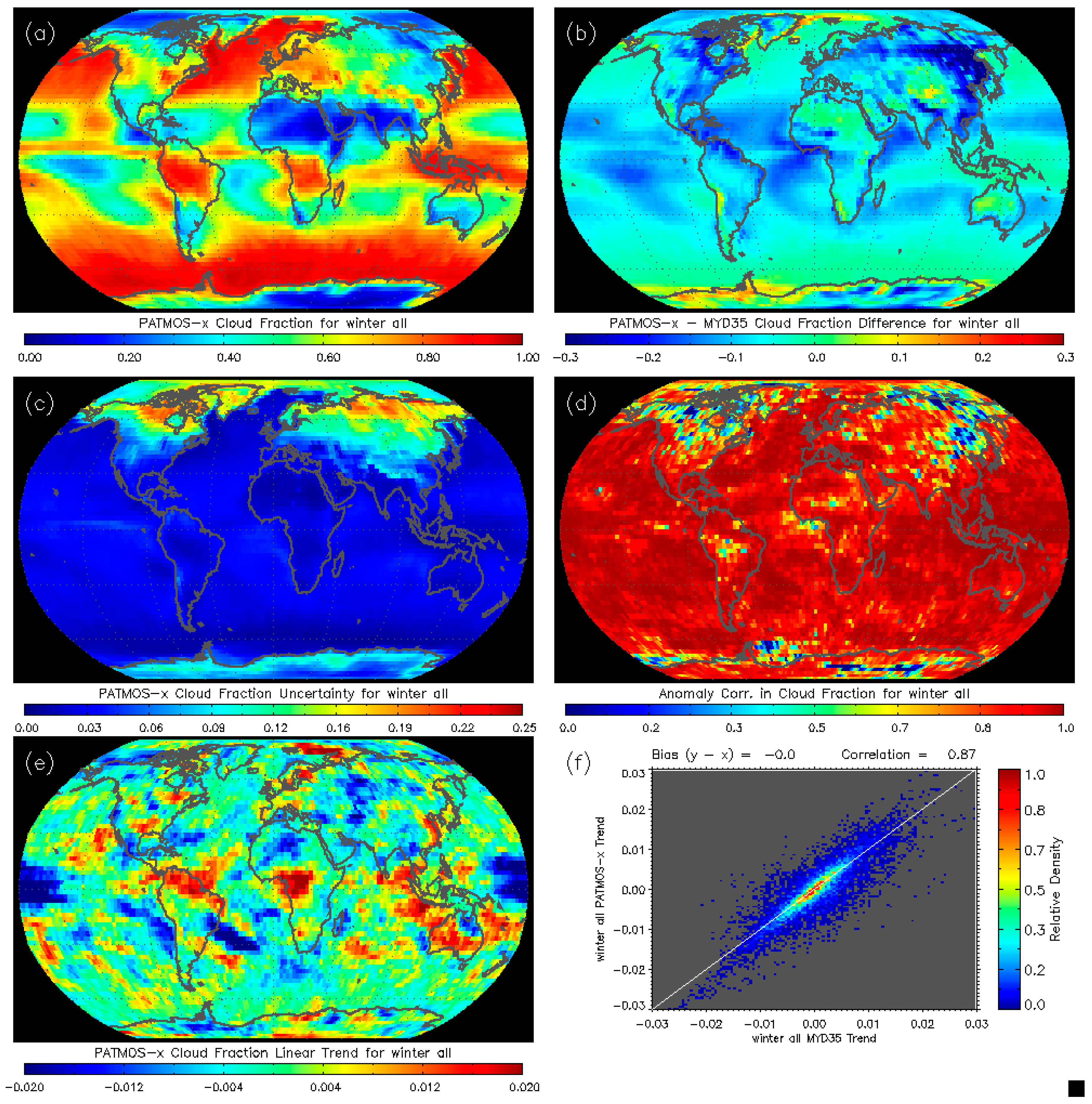
3.1. Comparison of MODIS PATMOS-x to NASA MODIS MYD35
3.2. Comparison of MODIS PATMOS-x to NASA CALIPSO CALIOP
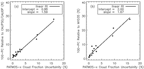
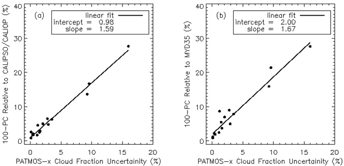
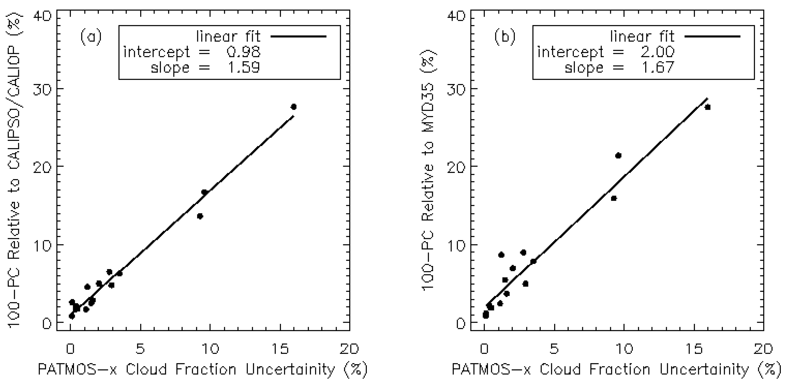
3.3. Verification of the PATMOS-x Cloud Fraction Uncertainty
3.4. Sensitivity of PATMOS-x Cloud Fraction to Prior Cloud Amount Assumptions
3.5. Sensitivity Based on Spectral Content
4. Conclusions
- For regions where the reported PATMOS-x cloud fraction uncertainty is less than 5%, the PATMOS-x and MYD35 cloud fraction annual anomaly correlations are high and the linear trends over 2003 to 2014 agree well.
- Relative to CALIPSO, PATMOS-x and MYD35 global cloud fractions generally agree within 2%, except for snow-covered land and nighttime Arctic and nighttime Antarctic surface types.
- Comparisons of the reported PATMOS-x cloud fraction uncertainty to direct estimates of error relative to CALIPSO or MYD35 reveal that the PATMOS-x cloud fraction uncertainties are 1.6 times too small but show a linear relationship.
- Being a naïve Bayesian technique, the PATMOS-x cloud fraction is dependent on the assumed surface-type-dependent climatological cloud fraction. Regions with low cloud and small cloud fractions over the ocean showed the most sensitivity to the climatological clouds, as did regions where the cloud fraction uncertainty was high (>10%).
- The cloud fraction trends from the naïve Bayesian PATMOS-x approach agreed well with those from the non-Bayesian MYD35 approach over most regions. This supports the idea that naïve Bayesian cloud detection approaches are suitable for multi-decadal satellite climate research.
- The PATMOS-x AVHRR results show little sensitivity to the spectral switch from AVHRR Ch3a to Ch3b. The PATMOS-x AVHRR cloud fractions are higher than those from MODIS and VIIRS in oceanic regions with low cloud amounts. The PC values also show little impact, except for the Antarctica region where the additional MODIS spectral information adds skill.
- In general, the PATMOS-x MYD02SSH/AVHRR results agree better with CALIPSO than the PATMOS-x AVHRR generated from NOAA-19/AVHRR/GAC data. These differences were small for most surface types. The larger differences occurred over snow and ice-covered surfaces where the radiometric differences between the AVHRR and the MODIS sensors are the largest.
Acknowledgments
Author Contributions
Conflicts of Interest
Abbreviations
| AVHRR | Advanced Very High Resolution Radiometer |
| AMSU | Advanced Microwave Sounding Unit |
| C6 | Collection 6 of the MODIS Science Team Products |
| CALIOP | Cloud–Aerosol Lidar with Orthogonal Polarization |
| CALIPSO | Cloud–Aerosol Lidar and Infrared Pathfinder Satellite Observations |
| CDR | Climate Data Record |
| DNB | Day Night Band |
| EOS | Earth Observing System |
| EUMETSAT | European Organization for the Exploitation of Meteorological Satellites |
| HIRS | High Resolution Infrared Sounder |
| JPSS | Joint Polar Satellite System |
| LAADSWEB | L1 and Atmosphere Archive and Distribution System |
| MODIS | Moderate Resolution Imaging Spectroradiometer |
| MYD021KM | Aqua MODIS 1-km Level-1b |
| MYD02SSH | Aqua MODIS 5-km sub-sampled Level-1b |
| NASA | National Aeronautics and Space Administration |
| NCEI | National Centers for Environmental Information |
| NESDIS | National Environmental Satellite Data and Information Service |
| NOAA | National Oceanic and Atmospheric Administration |
| PATMOS-x | Pathfinder Atmospheres Extended |
| PC | Proportion Correct |
| POES | Polar Orbiting Environmental Satellites |
| VIIRS | Visible Infrared Imaging Radiometer Suite |
References
- National Research Council. Committee on Climate Data Records from NOAA Operational Satellites. In Climate Data Records from Environmental Satellites; National Academies Press: Washington, DC, USA, 2004; p. 136. Available online: http://www.nap.edu/catalog/10944/climate-data-records-from-environmental-satellites-interim-report (accessed on 7 June 2016).
- IPCC. Summary for policymakers. In Climate Change 2013: The Physical Science Basis. Contribution of Working Group I to the Fifth Assessment Report of the Intergovernmental Panel on Climate Change; Stocker, T.F., Plattner, G.-K., Tignor, M., Allen, S.K., Boschung, J., Nauels, A., Xia, Y., Bex, V., Midgley, P.M., Eds.; Cambridge: New York, NY, USA, 2013. [Google Scholar]
- Heidinger, A.K.; Foster, M.J.; Walther, A.; Zhao, X. The pathfinder atmospheres–extended avhrr climate dataset. Bull. Am. Meteorol. Soc. 2014, 95, 909–922. [Google Scholar] [CrossRef]
- Stubenrauch, C.J.; Rossow, W.B.; Kinne, S.; Ackerman, S.; Cesana, G.; Chepfer, H.; Di Girolamo, L.; Getzewich, B.; Guignard, A.; Heidinger, A.; et al. Assessment of global cloud datasets from satellites: Project and database initiated by the GEWEX Radiation Panel. Bull. Am. Meteorol. Soc. 2013, 94, 1031–1049. [Google Scholar] [CrossRef]
- Karlsson, K.G.; Riihela, A.; Muller, R.; Meirink, J.F.; Sedlar, J.; Stengel, M.; Lockhoff, M.; Trentmann, J.; Kaspar, F.; Hollmann, R.; et al. CLARA-A1: A cloud, albedo, and radiation dataset from 28 yr of global AVHRR data. Atmos. Chem. Phys. 2013, 13, 5351–5367. [Google Scholar] [CrossRef]
- Heidinger, A.K.; Evan, A.T.; Foster, M.J.; Walther, A. A naive bayesian cloud-detection scheme derived from CALIPSO and applied within PATMOS-x. J. Appl. Meteorol. Climatol. 2012, 51, 1129–1144. [Google Scholar] [CrossRef]
- Karlsson, K.G.; Johansson, E. On the optimal method for evaluating cloud products from passive satellite imagery using CALIPSO-CALIOP data: Example investigating the CM SAF CLARA-A1 dataset. Atmos. Meas. Tech. 2013, 6, 1271–1286. [Google Scholar] [CrossRef]
- Minnis, P.; Sun-Mack, S.; Young, D.F.; Heck, P.W.; Garber, D.P.; Chen, Y.; Spangenberg, D.A.; Arduini, R.F.; Trepte, Q.Z.; Smith, W.L.; et al. CERES Edition-2 cloud property retrievals using TRMM VIRS and Terra and Aqua MODIS data-part I: Algorithms. IEEE Trans. Geosci. Remote Sens. 2011, 49, 4374–4400. [Google Scholar] [CrossRef]
- Stowe, L.L.; Davis, P.A.; McClain, E.P. Scientific basis and initial evaluation of the CLAVR-1 global clear cloud classification algorithm for the advanced very high resolution radiometer. J. Atmos. Ocean. Technol. 1999, 16, 656–681. [Google Scholar] [CrossRef]
- Nielsen, J.K.; Foster, M.; Heidinger, A. Tropical stratospheric cloud climatology from the PATMOS-x dataset: An assessment of convective contributions to stratospheric water. Geophys. Res. Lett. 2011, 38. [Google Scholar] [CrossRef]
- Evan, A.T.; Dunino, J.; Foley, J.A.; Heidinger, A.K.; Velden, C.S. New evidence for a relationship between Atlantic tropical cyclone activity and African dust outbreaks. Geophys. Res. Lett. 2006, 33. [Google Scholar] [CrossRef]
- Ackerman, S.; Heidinger, A.; Foster, M.; Maddux, B. Satellite regional cloud climatology over the great lakes. Remote Sens. 2013, 5, 6223–6240. [Google Scholar] [CrossRef]
- Foster, M.J.; Heidinger, A. Entering the era of +30-year satellite cloud climatologies: A north American case study. J. Clim. 2014, 27, 6687–6697. [Google Scholar] [CrossRef]
- Sun, B.M.; Free, M.; Yoo, H.L.; Foster, M.J.; Heidinger, A.; Karlsson, K.G. Variability and trends in U.S. Cloud cover: isccp, PATMOS-x, and CLARA-A1 compared to homogeneity-adjusted weather observations. J. Clim. 2015, 28, 4373–4389. [Google Scholar] [CrossRef]
- Foster, M.J.; Heidinger, A. Patmos-x: Results from a diurnally corrected 30-yr satellite cloud climatology. J. Clim. 2013, 26, 414–425. [Google Scholar] [CrossRef]
- Zhao, T.X.P.; Chan, P.K.; Heidinger, A.K. A global survey of the effect of cloud contamination on the aerosol optical thickness and its long-term trend derived from operational AVHRR satellite observations. J. Geophys. Res. Atmos. 2013, 118, 2849–2857. [Google Scholar] [CrossRef]
- Menzel, W.P.; Wylie, D.P.; Jackson, D.L.; Bates, J.J. Global cloud cover trends inferred from two decades of HIRS observations. Proc. SPOI 2005, 5658, 283–291. [Google Scholar]
- Frey, R.A.; Ackerman, S.A.; Liu, Y.; Strabala, K.I.; Zhang, H.; Key, J.R.; Wang, X. Cloud detection with MODIS. Part I: Improvements in the MODIS cloud mask for Collection 5. J. Atmos. Ocean. Technol. 2008, 25, 1057–1072. [Google Scholar] [CrossRef]
- Ackerman, S.A.; Strabala, K.I.; Menzel, W.P.; Frey, R.A.; Moeller, C.C.; Gumley, L.E. Discriminating clear sky from clouds with MODIS. J. Geophys. Res. Atmos. 1998, 103, 32141–32157. [Google Scholar] [CrossRef]
- Ackerman, S.A.; Holz, R.E.; Frey, R.; Eloranta, E.W.; Maddux, B.C.; McGill, M. Cloud detection with MODIS. Part II: Validation. J. Atmos. Ocean. Technol. 2008, 25, 1073–1086. [Google Scholar] [CrossRef]
- Roebeling, R.; Baum, B.; Bennartz, R.; Hamann, U.; Heidinger, A.; Thoss, A.; Walther, A. Evaluating and improving cloud parameter retrievals. Bull. Am. Meteorol. Soc. 2013, 94, Es41–Es44. [Google Scholar] [CrossRef]
- Young, S.A.; Vaughan, M.A.; Winker, D.M. Adaptive algorithms for the fully-automated retrieval of cloud and aerosol extinction profiles from calipso lidar data. In Proceedings of the 2003 IEEE International Geoscience and Remote Sensing Symposium (IGARSS '03), Toulouse, France, 21–25 July 2003; pp. 1517–1519.
- Laads Web Level 1 and Atmosphere Archive and Distribution System. Available online: https://ladsweb.nascom.nasa.gov (accessed on 7 June 2016).
- Barnes, W.L.; Pagano, T.S.; Salomonson, V.V. Prelaunch characteristics of the moderate resolution imaging spectroradiometer (MODIS) on EOS-AM1. IEEE Trans. Geosci. Remote Sens. 1998, 36, 1088–1100. [Google Scholar] [CrossRef]
- Maddux, B.C.; Ackerman, S.A.; Platnick, S. Viewing geometry dependencies in modis cloud products. J. Atmos. Ocean. Technol. 2010, 27, 1519–1528. [Google Scholar] [CrossRef]
- Ma, J.J.; Wu, H.; Wang, C.; Zhang, X.; Li, Z.Q.; Wang, X.H. Multiyear satellite and surface observations of cloud fraction over China. J. Geophys. Res. Atmos. 2014, 119, 7655–7666. [Google Scholar] [CrossRef]
- Liu, Y.; Ackerman, S.A.; Maddux, B.C.; Key, J.R.; Frey, R.A. Errors in cloud detection over the Arctic using a satellite imager and implications for observing feedback mechanisms. J. Clim. 2010, 23, 1894–1907. [Google Scholar] [CrossRef]
- Baum, B.A.; Menzel, W.P.; Frey, R.A.; Tobin, D.C.; Holz, R.E.; Ackerman, S.A.; Heidinger, A.K.; Yang, P. MODIS cloud-top property refinements for Collection 6. J. Appl. Meteorol. Climatol. 2012, 51, 1145–1163. [Google Scholar] [CrossRef]
- Heidinger, A.K. Abi cloud mask. In GOES-R Algorithm Theoretical Basis Document; 2011; p. 93. Available online: http://www.goes-r.gov/products/ATBDs/baseline/Cloud_CldMask_v2.0_no_color.pdf (accessed on 7 June 2016).
- Liu, Y.; Key, J.R.; Frey, R.A.; Ackerman, S.A.; Menzel, W.P. Nighttime polar cloud detection with MODIS. Remote Sens. Environ. 2004, 92, 181–194. [Google Scholar] [CrossRef]


| Sensor | Nominal Wavelengths (µm) of Channels Used in PATMOS-x Cloud Mask | |||||||||
|---|---|---|---|---|---|---|---|---|---|---|
| 0.65 | 0.86 | 1.38 | 1.6 | 3.75 | 6.7 | 8.5 | 11 | 12 | DNB | |
| AVHRR/3a | ✓ | ✓ | ✓ (day) | ✓ (night) | ✓ | ✓ | ||||
| AVHRR/3b | ✓ | ✓ | ✓ | ✓ | ✓ | |||||
| MODIS | ✓ | ✓ | ✓ | ✓ | ✓ | ✓ | ✓ | ✓ | ✓ | |
| VIIRS | ✓ | ✓ | ✓ | ✓ | ✓ | ✓ | ✓ | ✓ | ✓ | |
| PATMOS-x or MYD35 | ||
|---|---|---|
| CALIPSO | Clear | Cloudy |
| Clear | a | b |
| Cloudy | c | d |
| Region | Cloud Fractions | PC 0/100 Filter | PC 50/50 Filter | ||||||||
|---|---|---|---|---|---|---|---|---|---|---|---|
| CAL | PM | MYD | A/C | P/C | M/C | P/M | A/C | P/C | M/C | P/M | |
| Global | 66 | 63 | 64 | 98 | 99 | 99 | 99 | 89 | 91 | 90 | 95 |
| Ocean | 70 | 67 | 70 | 99 | 100 | 100 | 100 | 89 | 91 | 91 | 97 |
| Water | 67 | 65 | 65 | 99 | 100 | 99 | 100 | 91 | 93 | 93 | 97 |
| Land | 60 | 54 | 55 | 98 | 99 | 99 | 99 | 86 | 88 | 88 | 95 |
| Snow | 73 | 69 | 75 | 96 | 96 | 98 | 97 | 88 | 88 | 89 | 86 |
| Arctic | 78 | 72 | 72 | 91 | 95 | 96 | 99 | 82 | 90 | 90 | 91 |
| Antarctic | 79 | 78 | 74 | 98 | 99 | 98 | 98 | 94 | 91 | 89 | 90 |
| Desert | 36 | 31 | 28 | 99 | 99 | 99 | 100 | 93 | 90 | 89 | 94 |
| Region | Cloud Fraction | PC 0/100 Filter | PC 50/50 Filter | ||||||||
|---|---|---|---|---|---|---|---|---|---|---|---|
| CAL | PAT | MYD | A/C | P/C | M/C | P/M | A/C | P/C | M/C | P/M | |
| Global | 72 | 66 | 69 | 95 | 96 | 97 | 96 | 84 | 88 | 88 | 89 |
| Ocean | 76 | 71 | 75 | 98 | 99 | 99 | 99 | 85 | 90 | 90 | 93 |
| Water | 77 | 72 | 77 | 98 | 98 | 99 | 99 | 90 | 91 | 92 | 92 |
| Land | 61 | 52 | 62 | 90 | 97 | 97 | 96 | 81 | 91 | 91 | 89 |
| Snow | 77 | 60 | 67 | 86 | 90 | 91 | 90 | 76 | 79 | 81 | 78 |
| Arctic | 77 | 66 | 67 | 89 | 95 | 90 | 92 | 78 | 85 | 81 | 84 |
| Antarctic | 76 | 71 | 57 | 82 | 73 | 85 | 66 | 72 | 67 | 74 | 59 |
| Desert | 23 | 17 | 24 | 96 | 97 | 97 | 96 | 89 | 93 | 90 | 90 |
| Sensor | Proportional Correct (%) for P/C Using 50/50 Filter | |||||||
|---|---|---|---|---|---|---|---|---|
| Global | Ocean | Water | Land | Snow | Arctic | Antarctica | Desert | |
| AVHRR/3a | 88 | 91 | 91 | 88 | 80 | 80 | 75 | 91 |
| AVHRR/3b | 89 | 91 | 93 | 89 | 82 | 83 | 77 | 91 |
| MODIS | 87 | 89 | 92 | 86 | 79 | 79 | 81 | 91 |
| VIIRS | 87 | 90 | 93 | 87 | 76 | 76 | 80 | 93 |
| NOAA-19-AVHRR/3b | 86 | 87 | 91 | 84 | 81 | 75 | 73 | 91 |
© 2016 by the authors; licensee MDPI, Basel, Switzerland. This article is an open access article distributed under the terms and conditions of the Creative Commons Attribution (CC-BY) license (http://creativecommons.org/licenses/by/4.0/).
Share and Cite
Heidinger, A.; Foster, M.; Botambekov, D.; Hiley, M.; Walther, A.; Li, Y. Using the NASA EOS A-Train to Probe the Performance of the NOAA PATMOS-x Cloud Fraction CDR. Remote Sens. 2016, 8, 511. https://doi.org/10.3390/rs8060511
Heidinger A, Foster M, Botambekov D, Hiley M, Walther A, Li Y. Using the NASA EOS A-Train to Probe the Performance of the NOAA PATMOS-x Cloud Fraction CDR. Remote Sensing. 2016; 8(6):511. https://doi.org/10.3390/rs8060511
Chicago/Turabian StyleHeidinger, Andrew, Michael Foster, Denis Botambekov, Michael Hiley, Andi Walther, and Yue Li. 2016. "Using the NASA EOS A-Train to Probe the Performance of the NOAA PATMOS-x Cloud Fraction CDR" Remote Sensing 8, no. 6: 511. https://doi.org/10.3390/rs8060511
APA StyleHeidinger, A., Foster, M., Botambekov, D., Hiley, M., Walther, A., & Li, Y. (2016). Using the NASA EOS A-Train to Probe the Performance of the NOAA PATMOS-x Cloud Fraction CDR. Remote Sensing, 8(6), 511. https://doi.org/10.3390/rs8060511