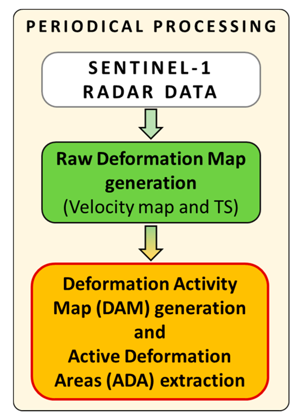
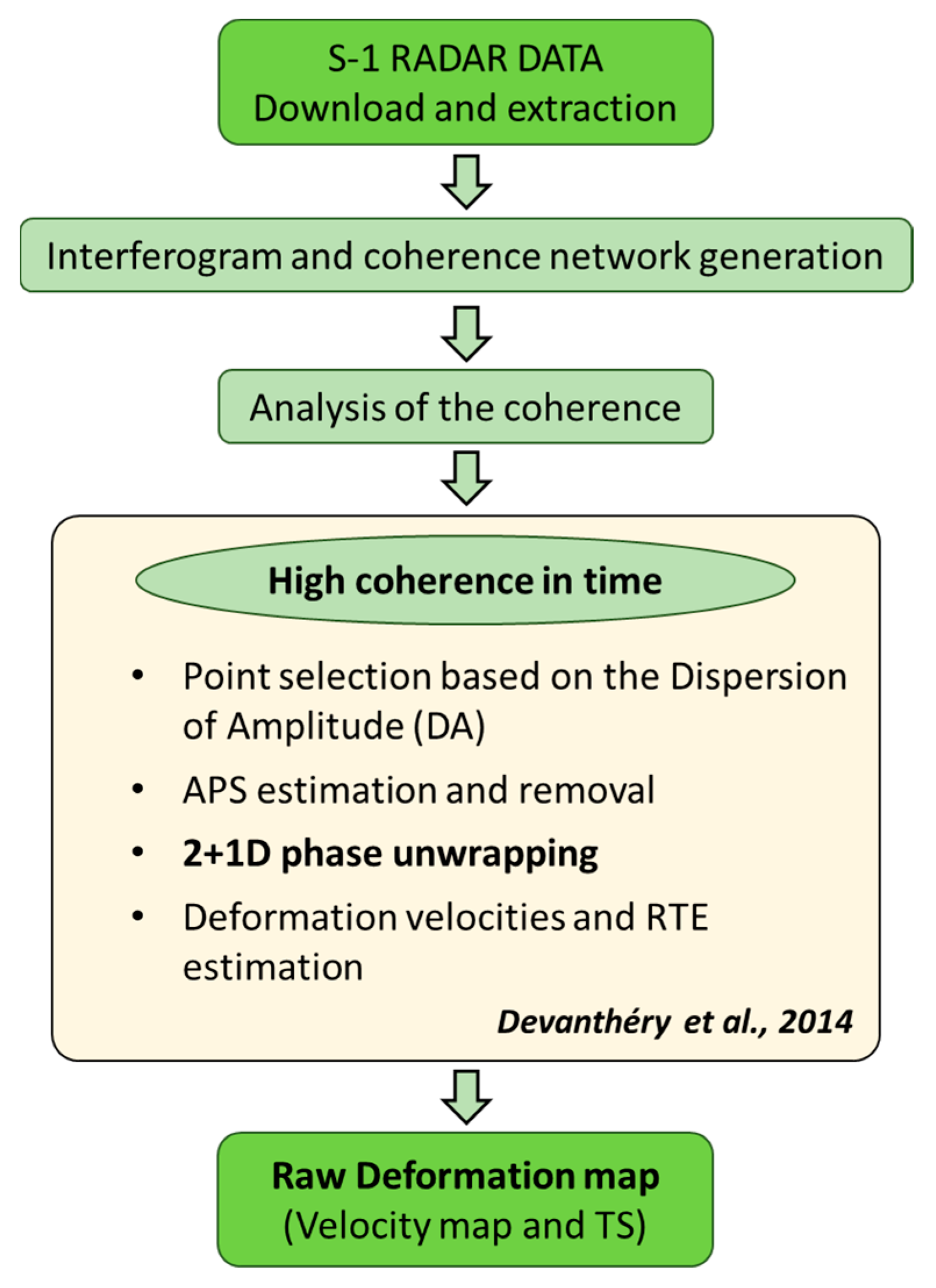
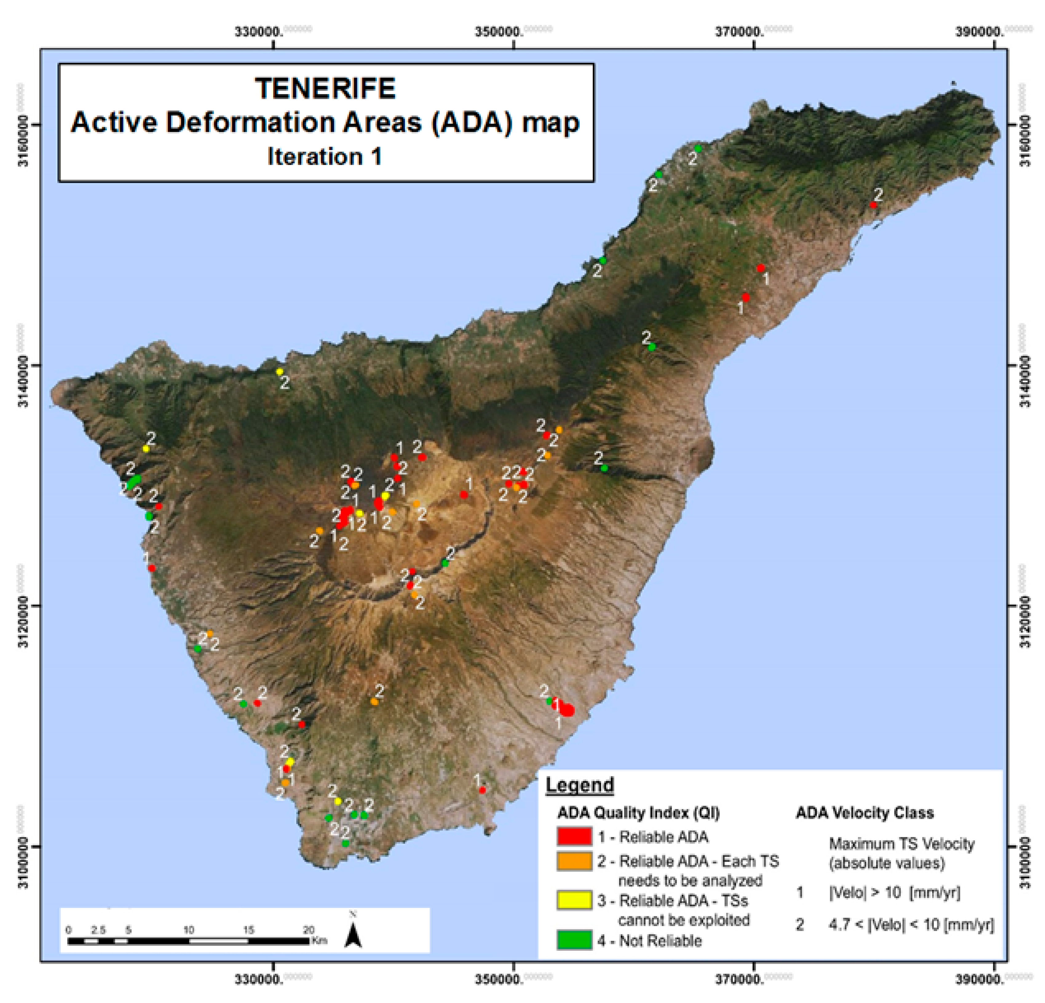
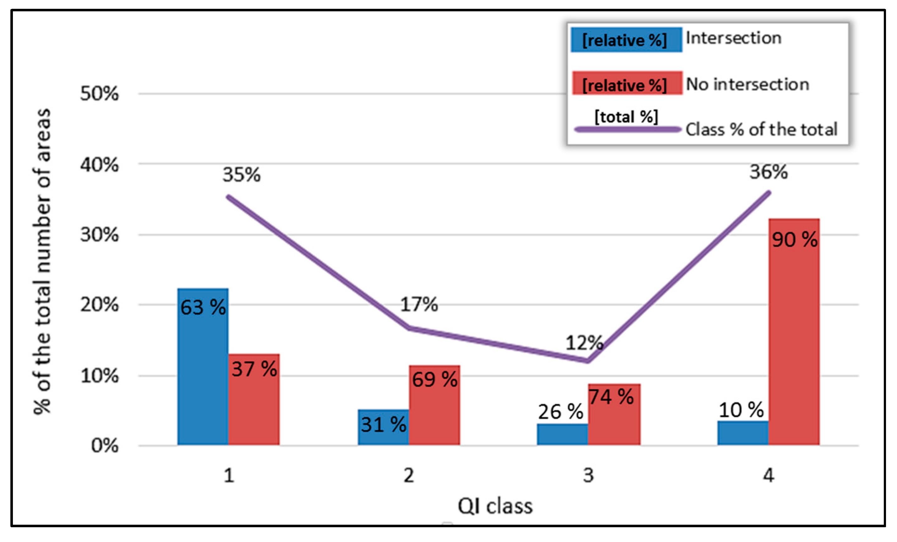
In this section, the procedure to derive the DAM and the ADA maps is described. The proposed procedure can be applied to the data acquired by any satellite SAR sensor. However, it provides the best performances with the S-1 characteristics.
All the deformation values included in the output maps are estimated along the satellite Line of Sight (LOS) direction. The procedure is designed to be periodically processed to have a continuous update of the products and thus a continuous input of regional-scale deformation maps for the authorities to detect potential hazards or to decide more focused analysis in critical areas.
2.2. Deformation Activity Map and Active Deformation Areas Extraction
This block is aimed at obtaining both the final Deformation Activity Map (DAM), which is the filtered version of the raw deformation map (RDM), and the Active Deformation Areas (ADA) map, which is the main product of the procedure. The main goal is to identify and monitor, over wide areas, the most critical deformations to provide the Civil Protection authorities with the capacity to perform prevention and mitigation actions. Therefore, the three main aspects that have to characterize the final maps are: (i) the readability; (ii) the reliability; and (iii) the regional-to-local scale. The main constraining factors to achieve these goals are the spatio-temporal noise of the deformation map and the high number of PSs which in some cases can lead to wrong interpretations.
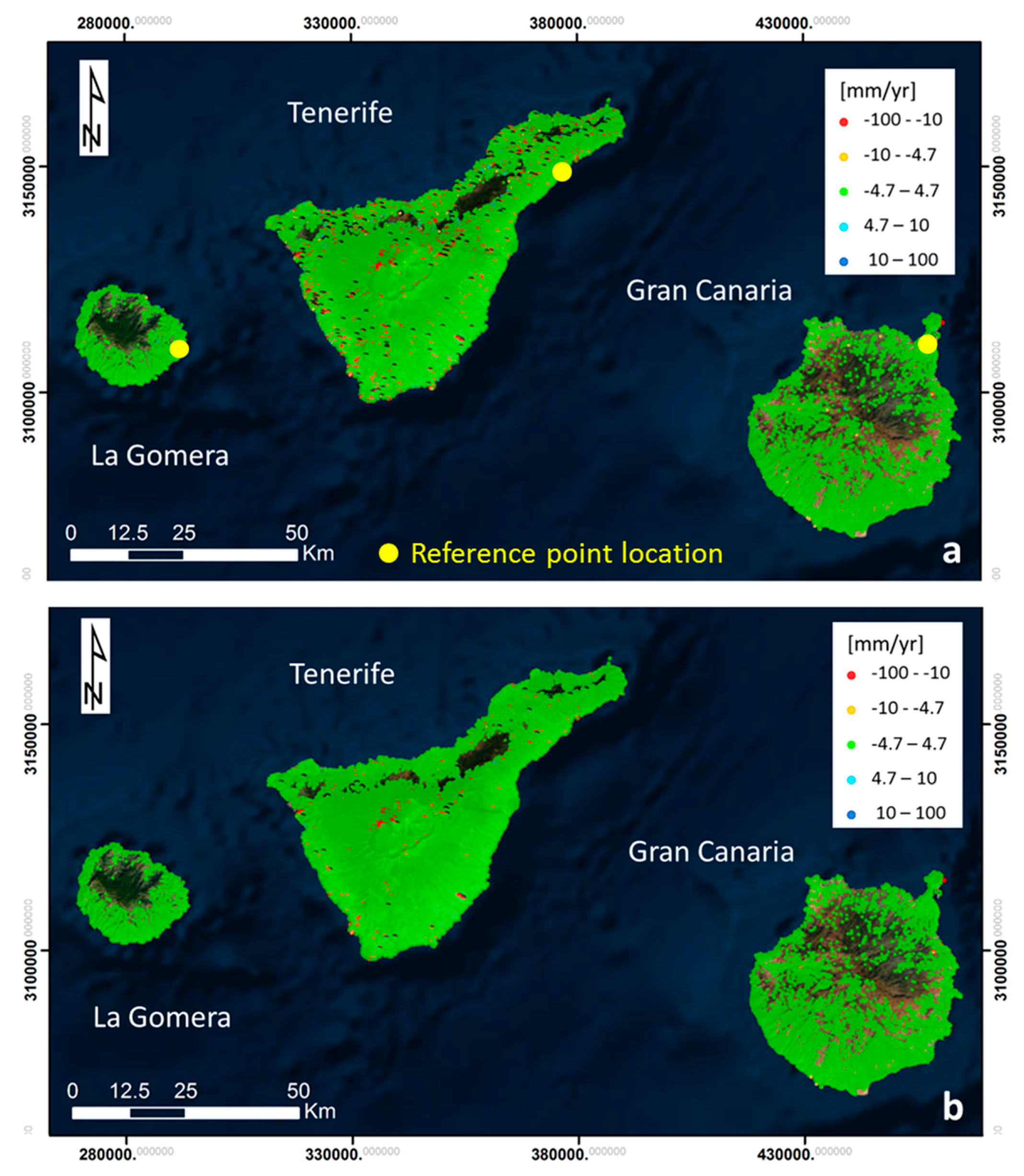
A key parameter of this block is the assessment of the general noise level (sensitivity) of the RDM. In this research, the sensitivity has been evaluated using the standard deviation (σmap) of the RDM velocity values. A stability threshold of 2σmap is set to distinguish the active points, those where we measure movements, from those we do not. A point is considered moving if |v| > 2σmap, where |v| is the absolute velocity value of the point. It is worth to underline that the points classified as “stable” can be truly stable as well as instable points, with a not detectable movement. To simplify the readability, we call “stable” all the points with the absolute LOS velocity below the stability threshold. As example, in the Canary Island test site, the stability threshold has been set as ±4.7 mm/year.
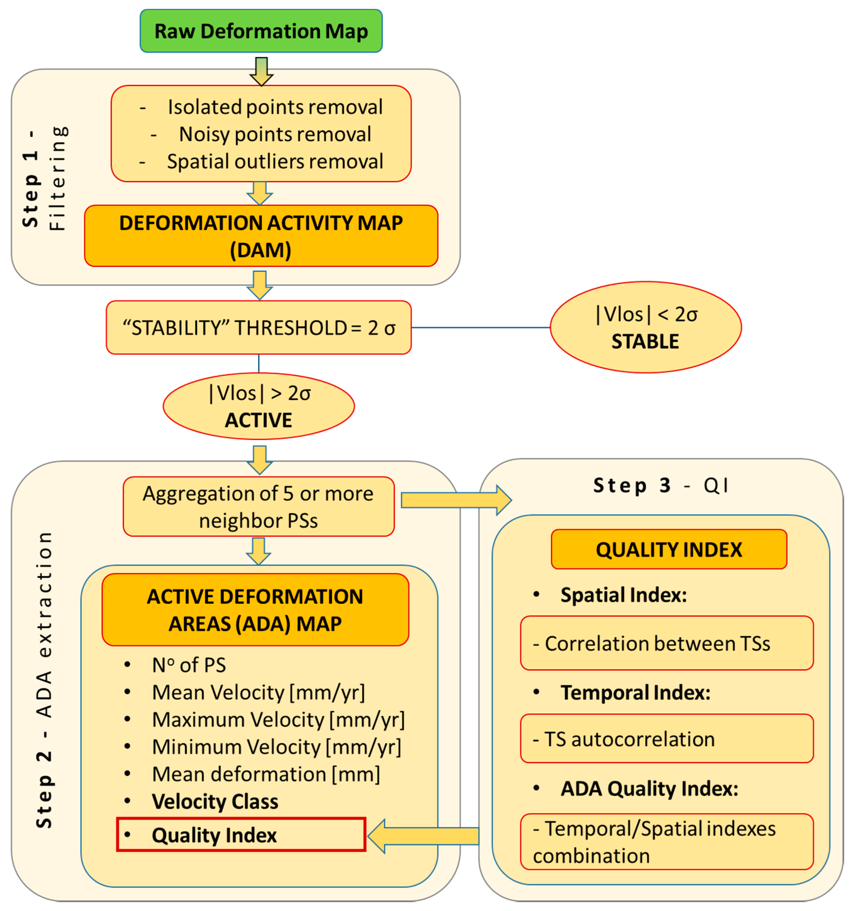
This block can be summarized in three main steps (
Figure 3): (i) filtering of the RDM; (ii) automatic extraction of the more reliable and relevant active areas (ADA); and (iii) Quality Index (QI) attribution to each ADA.
(i) Filtering of the raw deformation map
This action aims to filter the RDM obtained in block 1. The final point selection has been based on two different criteria: (i) the standard deviation of the 2+1D phase unwrapping residues (σres); and (ii) a spatial criterion based on the variability of a point with respect its neighbors. The first one is used to remove points susceptible to be affected by phase unwrapping errors. The used threshold for the σres is 2.4 rad (approximately 1 cm). We have selected this relatively high threshold in order to keep the maximum number of measurements. Regarding the spatial criterion, it is used to clean sparse measurements (isolated points) and points with strong discrepancy with respect its neighbors (outliers). The filtering is window based. The used window has a radius of 2 times the data resolution (e.g., around 80 m in Canary Island).
The filtering criteria are: (i) eliminate points without neighbors inside the window; and (ii) eliminate moving points without more than one moving neighbors inside the window. It is worth noting that the eliminated points can be real moving points related to a geohazard, like for example a landslide. However, an isolated point can be related to several factors including noise. In this context, we accept to lose information about few phenomena in order to highly reduce the general level of noise and simplify the readability of the map.
(ii) Automatic extraction of the more reliable and relevant active areas (ADA)
The aim of the ADA map generation is to perform a rapid identification of the most reliable active deformation areas. The final map has to represent a clear input to be validated and integrated with other data (e.g., geohazard inventories, ground truth information, etc.) in order to determine the nature of the deformation and thus to generate the Geohazard Activity Map.
The ADA map has been by using an evolution of the approaches proposed by [
37,
38,
39,
40]. The main input is the filtered deformation velocity map obtained in Step (i). Only the moving points (with |
v| > 2σ
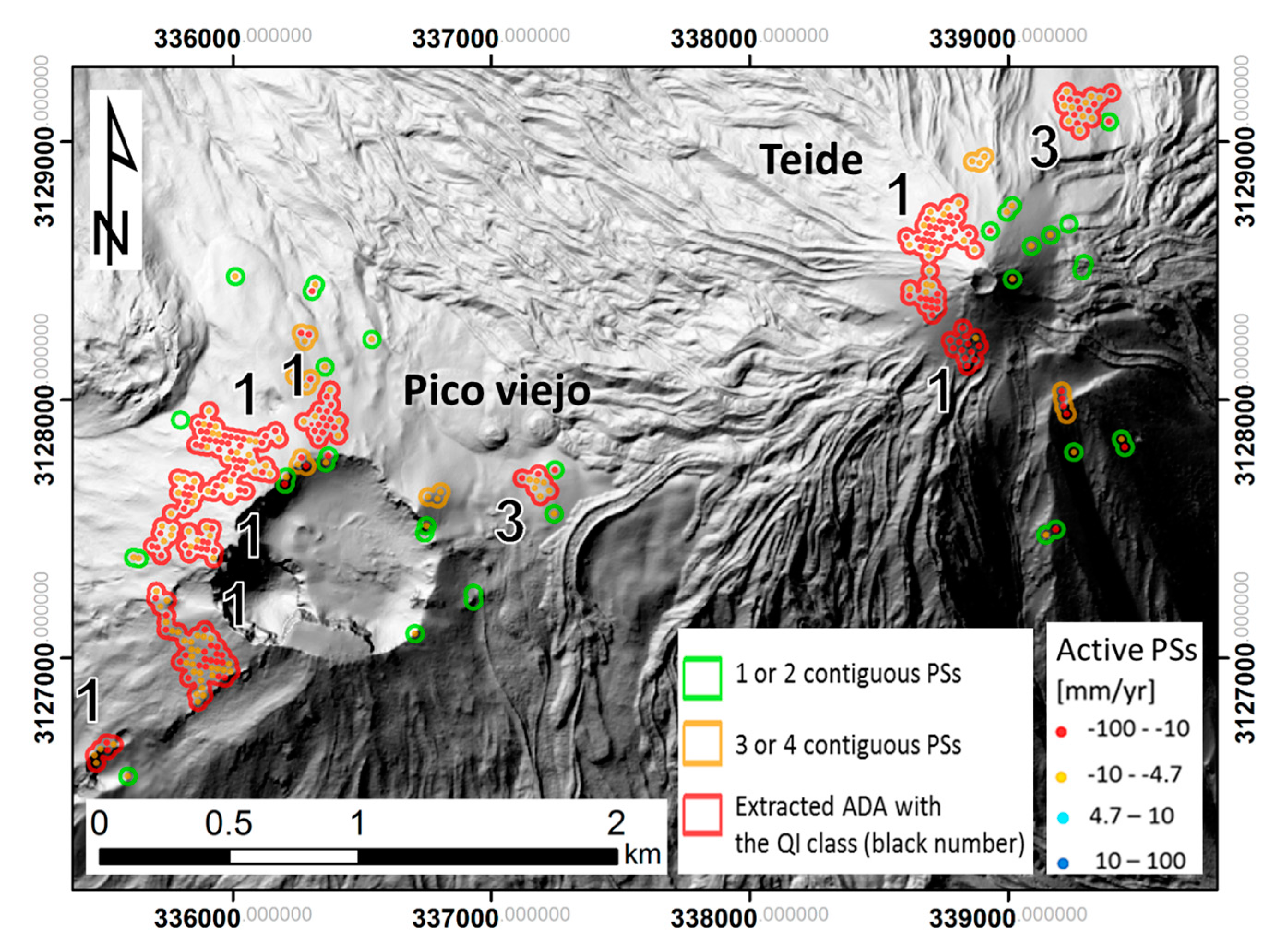
map) are selected. Then, from this subset of points (PSm), groups of at least five neighbor PSs, sharing their influence area, are aggregated in polygons representing the Active Deformation Areas (ADA). To define the influence area of every PS we consider the approximated footprint of the PSs. For example, in Canary Island test site, the PS area is of 28 m by 40 m. Then we calculate the radius of the circle inscribing the PS area (40 m by 40 m in the Canary Island Site) and we multiply it by a factor of 1.3 to ensure that neighboring pixels are selected. If the grouped PSs are less than five, they are considered to represent a non-significant deformation for a regional scale map.
Finally, for each ADA, the following parameters are estimated:
- -
Number of aggregated active points (APs).
- -
Mean, maximum and minimum values of the APs velocities.
- -
Mean value of the APs accumulated deformations. To avoid strong influence of atmospheric or digital elevation model error effects, we estimate the final accumulated deformation as the average of the accumulated values of the last four acquisition times of all the APs of the ADA.
- -
Velocity class, which is a classification of the ADA as a function of its maximum velocity (vm). The class is 1 if |vm| > 1 cm/year or 0 if 2σmap < |vm| < 1 cm/year.
- -
Quality Indexes, which are explained in the following lines.
(iii) Quality index attribution to each ADA
Although the ADA map is based on filtered data, the automation of the process needs a final quality assessment for each single ADA. The noise level of the TSs and thus the robustness of the deformation estimations vary significantly pointwise. This step describes an implemented Quality Index (QI) that provides an estimation of the noise level of the ADA. This QI is a key parameter to properly interpret the ADA map.
The QI is based on the evaluation of two parameters for each ADA: the noise of each AP time series is evaluated and the spatial homogeneity of the estimated deformations in time is considered (i.e., consistency between AP time series). Hence, each ADA is characterized by a temporal noise index (TNI) and a spatial noise index (SNI) that are used to derive the final QI.
• Temporal Noise Index (TNI)
To attribute the TNI, for each APs the first order autocorrelation (ρt,t−1) of its TS is evaluated. The first order autocorrelation allows evaluating the temporal noise degree for both linear and nonlinear deformation trends. The autocorrelation coefficient ranges from 0 to 1, where 0 means the prevalence of noise over the deformation trend. The temporal index (TNI) is a four-class classification of the ADA based on the median value (Med(ρ)) between the TS autocorrelation coefficients, it varies from 1 to 4, where 1 corresponds to a high Med(ρ) and 4 to a very low Med(ρ).
To find a relationship between the autocorrelation coefficient and the noise level, a simulation was performed on a set of 20 TSs characterized by a linear trend (b) and random noise (ϵ):
where b = velocity in (mm/day), x = 0, 12, 24, 36,…, 468 (days) is the 12 days spaced time series. The random noise was characterized by a normal distribution. For each velocity, we tested different levels of noise by setting the standard deviation of the simulated random noise. Since the autocorrelation also depends on the number of sampling (i.e., on the length of the TS and the revisit time), our simulation was calculated over 468-day time series (almost one year and half) with temporal steps of 12 days. This period corresponds to the temporal window used to generate the deformation maps in our test site (Canary Islands).
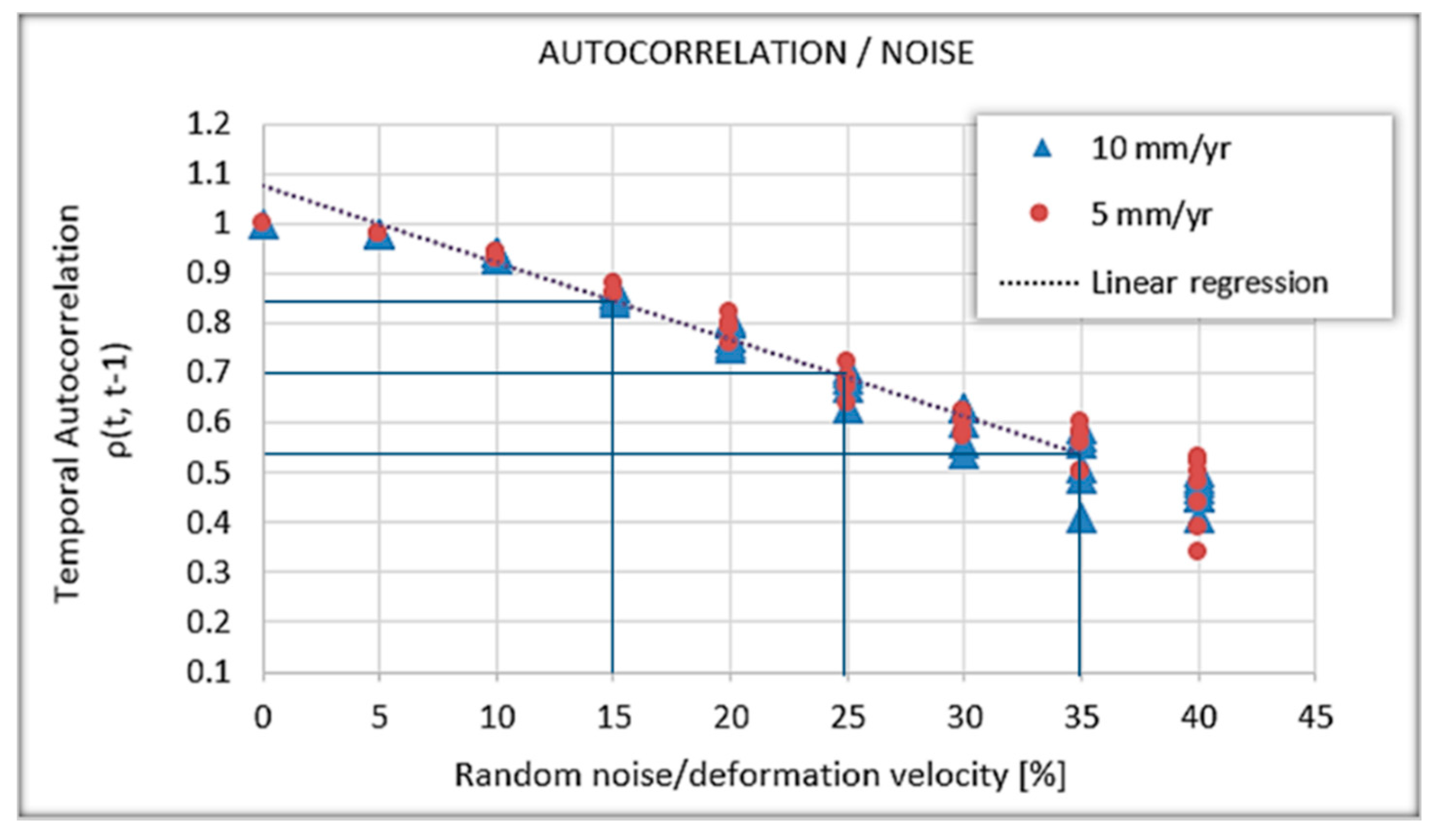
Figure 4 shows the results of the two simulations performed with the velocities of 5 and 10 mm/year. The plotted values represent the median value of the set of TSs autocorrelation coefficients calculated for each tested noise level. By expressing the noise level in terms of percentage of the velocities, the relationship can be approximated by the linear regression of the whole data resulted by the simulation.
It is worth mentioning that this is a simplified model, helpful to evaluate the physical meaning of the thresholds. Note that, for equal noise level, the autocorrelation coefficient changes with temporal sampling. Therefore, the thresholds can change, depending on the study case, if both the Sentinel-1A and Sentinel-1B images are used (six-day revisit time).
The
ρt,t−1 values of 0.53, 0.70 and 0.84, respectively, corresponding to the 35%, 25% and 15% of noise with respect to the velocities (
Figure 4 and
Table 1), were chosen as thresholds for the four classes of TNI.
• Spatial Noise Index (SNI)
The aim of the SNI estimation is to evaluate the spatial consistency of the detected ADA, i.e., to quantify how the PSs composing an ADA evolve with a similar trend. We assume that all the TSs of the same ADA belong to the same deformation phenomena. Thus, we expect different magnitude of the detected movements, but a spatial correlation between their temporal evolutions. With this aim, for each ADA the correlation coefficient between all the possible pairs of TSs are calculated (
CORR(Xi,Yj), where
i,
j represents all the possible pair combinations of the APs and
Xi and
Yj are their respective TSs. The spatial index (SNI) is a four-class classification of the ADA based on the median value (
Med(
CORR)) of all the ADA’s TSs pairs correlation values. It varies from 1 to 4 where 1 corresponds to a high
Med(
CORR) and 4 to a very low
Med(
CORR). The classification thresholds (
Table 2) have been set on the statistical distribution of the results, specifically the values corresponding to the quartiles that have been chosen.
• ADA Quality Index (QI)
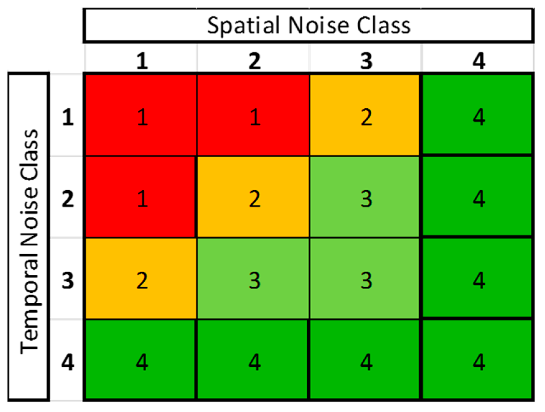
The global QI is derived from the combination of both the TNI and the SNI, and measures the degree of reliability of each detected ADA. The numerical classes (QI) assigned to each TNI-SNI combination are represented by the matrix shown in
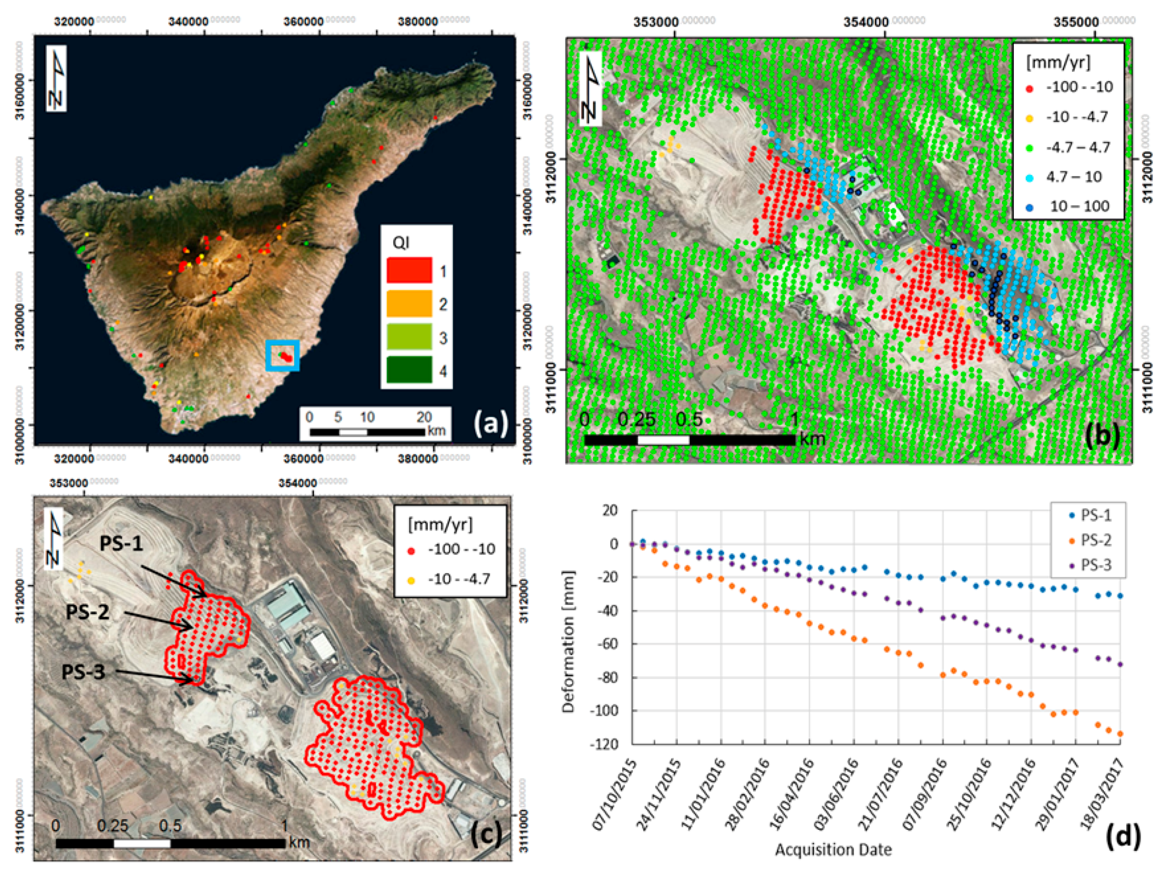
Figure 5. The QI ranges from Class 4, which is the noisiest one, to Class 1, which represents the ADA characterized by very high quality time series (TS). More in detail: Class 4 represents a not reliable ADA; Class 3 means reliable ADA but TS that cannot be exploited; Class 2 means reliable ADA, but a further analysis of the TS is recommended; and Class 1 means reliable ADA and TS.
