1. Introduction
The determination of the location and orientation of a straight line road is a fundamental task for many computer vision applications such as road network extraction [
1,
2,
3,
4,
5,
6,
7,
8,
9,
10,
11,
12,
13,
14,
15,
16,
17,
18,
19,
20,
21,
22,
23], image registration [
4],visual tracking [
5], robot autonomous navigation [
6], hyperspectral image classification [
7,
8], Global Navigation Satellite System(GNSS) [
9,
10], unmanned aerial vehicle images [
11], and sports video broadcasting [
12,
13]. A Hough transform (HT) [
14,
15,
16] is one of the very typical methods and has been widely applied to computer processing, image processing, and digital image processing. It transforms the problem of a global detection in a binary image into peaks detection in a Hough parameter space. Dozens of HT extensions have been developed for solving straight line road detection problem. And particularly, these methods can be divided into the following four groups: generalized HT (GHT) [
17,
18,
19,
20,
21], randomized HT (RHT) [
22,
23,
24,
25], probabilistic HT (PHT) [
26,
27,
28,
29], and fuzzy HT (FHT) [
30,
31,
32].
Generalized HT (GHT) [
17,
18,
19,
20,
21] detects arbitrary object curves (i.e., shapes having no or complex analytical form) by transforming the curves in image space into a four dimensional parameter space. For example, Lo et al. [
18] developed a perspective-transformation-invariant GHT (PTIGHT) by using a new perspective reference table (PR-table) to detect perspective planar shapes. Ji et al. [
19] proposed fuzzy GHT by using fuzzy set theory to focus the vote peaks to one point. Yang et al. [
20] proposed polygon-invariant GHT (PI-GHT) by exploiting the scale-and rotation invariant polygon triangles characteristic to accomplish High-Speed Vision-Based Positioning. Xu et al. [
21] developed robust invariant GHT (RIGHT) based on a robust shape model by utilizing an iterative training method.
Randomized Hough transform (RHT) [
22,
23,
24,
25] reduces the calculation and storage by using random sampling in image space, converging mapping and dynamic storage. Lu et al. [
23] proposed an iterative randomized HT (IRHT) by the iteration to gradually reduce the target area from the entire image to the region of interest. Jiang [
24] determined sample points and candidate circles by probability sampling and optimized methods to avoid false detection. Lu et al. [
25] developed a direct inverse RHT (DIRHT) by incorporating inverse HT with RHT, this method is able to enhance the target ellipse in strong noisy images.
Probabilistic Hough transform (PHT) [
26,
27,
28,
29] defines a Hough transform in a mathematically “correct” form with a likelihood function in the output parameters. Matas et al. [
27] proposed Progressive PHT (PPHT) utilized the difference in the fraction of votes to greatly reduce the amount of calculation of line detections. Galambos et al. [
28] controlled the vote process by gradient information to improve the performance of PPHT. Qiu and Wang [
29] proposed an improved PPHT by exploiting segment-weighted voting and density-based segment filtering to improve accuracy rate.
Fuzzy Hough transform (FHT) [
30,
31,
32] finds the target shapes in noisy images by fitting data points approximately. Basak and Pal [
31] utilized gray level images in FHT (gray FHT) to process the shape distortion. Pugin and Zhiznyakov [
32] proposed a new method of filter or fusion of straight lines after performing FHT and thus avoiding detecting unnecessary linear features.
Although Hough transform and its many variants have achieved better results, it is still a great challenge to develop a low computational complexity and time-saving HT algorithm. In this paper, we propose a new method based on a generalized HT (i.e., Radon transform) and apply it for straight road detection in remote sensing images. We adopt a dictionary learning method [
33] to approximate the Radon transform. The proposed approximation method has two significant contributions: (1) our method treats Radon transform as a linear transform, which greatly reducing the computational complexity; and (2) linear transformation makes it possible to realize parallel implementation of the Radon transform for multiple images, which can save time. To evaluate the proposed algorithm, we conduct extensive experiments on the popular RSSCN7 database for straight road detection. The experimental results demonstrate that our method is superior to the traditional HT algorithm in terms of accuracy and computing complexity.
The rest of this paper is arranged as follows.
Section 2 briefly reviews the related works including the Hough transform and Radon transform.
Section 3 presents the dictionary learning method to approximate the Radon transform.
Section 4 describes the extensive experiments and discusses the experimental results. Finally,
Section 5 gives some conclusions.
2. Related Work
In this section, we review some related works including Hough transform and Radon transform.
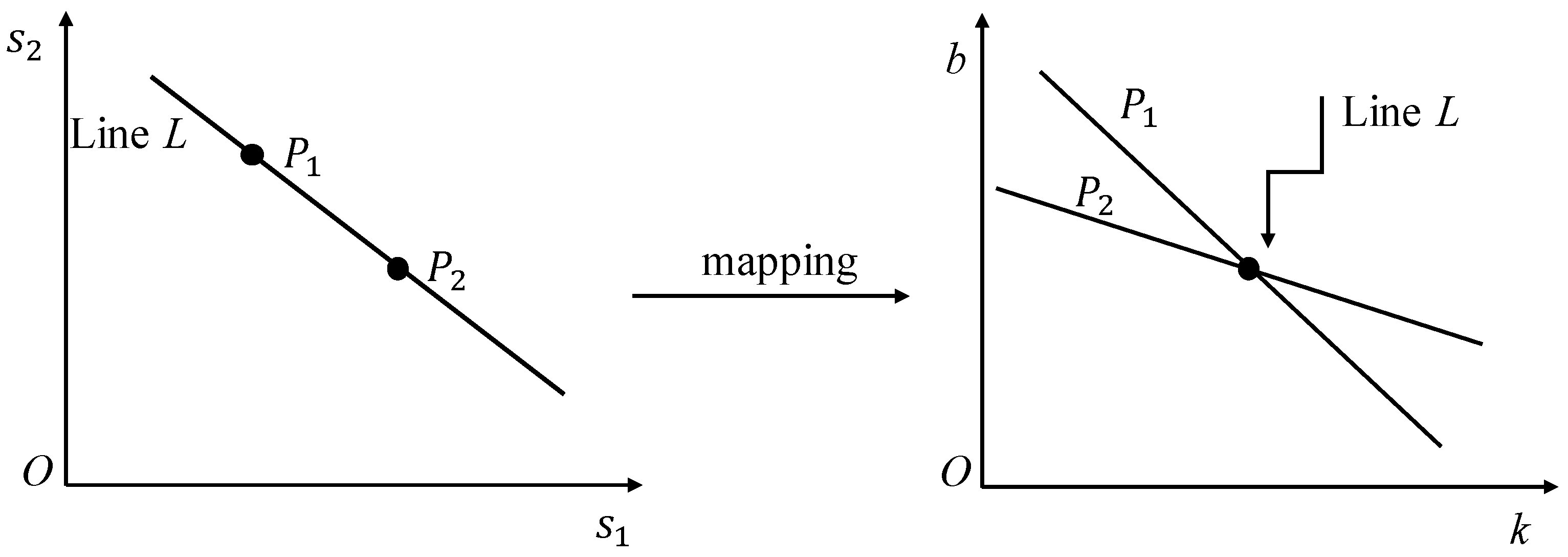
A Hough transform [
14,
15,
16] detects shape in binary images by using an array named parameter space. Each point in binary images votes for the parameters space. The highest values of votes in the parameter space represent a parameter shape with the same linear features in the original image. Generally, linear features of a straight line on two dimensional plane
are parameterized by the slope
and intercept
. Each point of a straight line will focus on one point in the
parameter space (
Figure 1).
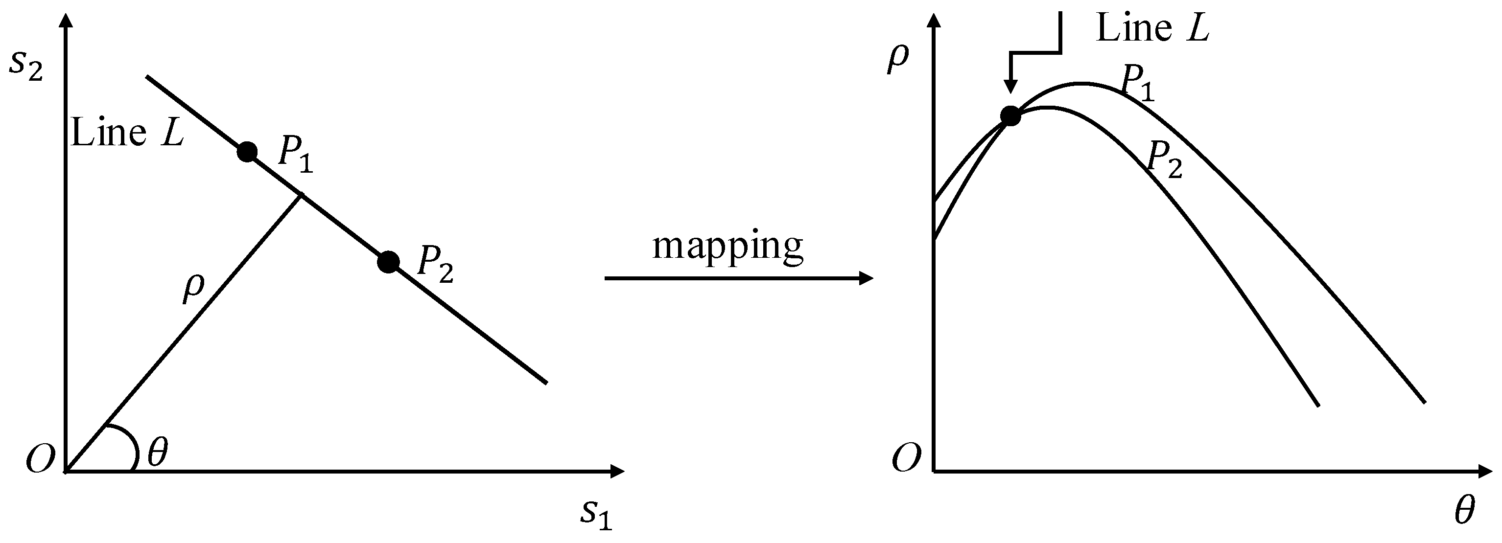
However, when the values of parameters are infinite (i.e.,
), the parametrization of a straight line exists a singularity. Duda and Hart [
34] proposes that straight lines can be parameterized by
(
Figure 2). And the mapping relations between image point
and
parameter space satisfy the following:
Considering that a Hough transform can only be used for binary images, a Radon transform extends this concept to the problem of straight line detection in grayscale images [
35]. If we denote
as an image on a two-dimensional Euclidean plane space, the Radon transform
of image
can be expressed as follows [
36]:
where
is the Dirac delta function,
is the Radon operator,
is the grayscale value of the point of
,
is the distance between the origin and the vertical of straight line, and
is the angle between the normal of straight line and the
axis. Each point
can be mapped into a sinusoidal curve in the parameterized space, and a single point
in the parameter space can be used to represent a line in image space.
The inverse Radon transform is defined as
where
is the Radon operator,
is the Fourier transform of
at angle
. In addition, the Formulas (3) and (4) are the filtered back projection algorithm which is introduced to compute the inverse Radon transform.
3. Dictionary Learning Based Radon Transform
In this section, we introduced a dictionary learning method to approximate the Radon transform. Specifically, we use linear transform to approximate the discretized form of Formula (3) in practice. The relationship between the discretized parameter space image
and the discretized image data
can be defined as [
37]:
where
is the discrete inverse Radon operator,
denotes the vectorized
, and
denotes the vectorized
.
In this paper, we employ a dictionary learning method to obtain the matrix
. Suppose the
training samples is
, where
denotes the vectorized
.
, and
denotes the vectorized
. Our purpose is to learn a dictionary
based on Equation (5):
Since
is not a square matrix, matrix
can be calculate by the least squares method through minimizing the following objection function:
where
denotes the 2-norm of
. By minimizing the objective function (7), we have
or
since matrix
or
may be a singular matrix or approach a singular matrix, we add a damping factor
(with range from 0.1 to 1) to ensure the stability of numerical value:
or
where matrix
is the transpose of the matrix
and
is a unit matrix.
Hence, the Radon transform of an image can be treated as a two matrix multiplication (i.e., linear transform):
Since
is not a square matrix, we can obtain the value of
by minimizing the following target function:
we have
or
Similarly, to ensure the stability of a numerical value, we add a damping factor
.
or
where matrix
is the transpose of the matrix
.
Our method treats a Radon transform as a linear transform, which can be realized by parallel computation of the Radon transform for multiple images:
or
The advantages of our solution is two-fold. Firstly, the transform (5) of the Radon operator makes it convenient and reasonable to leverage the performance by adding some special regularizations. For example, we can incorporate our objective function (5) into the regularization framework:
where
is a regularization term which includes norm regularizer terms, log regularizer term, etc. Norm regularization terms take the form of
for
- regularization,
for
- regularization,
for
- regularization, etc. The log regularization term is in the form of
. We will verify the effect of adding regularization items in the future work.
Secondly, the linear transformation makes it possible to detect a straight line road of multiple images at one time, which will significantly reduce the time consuming aspect of this process.
4. Experiments and Discussion
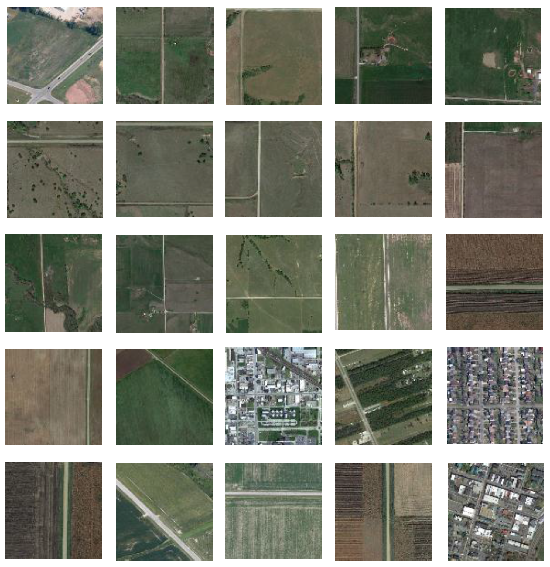
In order to evaluate the performance of our method, we implement extensive experiments on RSSCN7 [
38]. The RSSCN7 database is a remote sensing database which was issued in 2015, and the size of each remote sensing image is
pixels. There are 2800 remote sensing scene images in the RSSCN7 database, and they are from seven typical scene categories, which are a grassland, forest, farmland, parking lot, residential region, industrial region, river and lake. In this paper, we selected 170 remote sensing images with a straight line road to verify the proposed algorithm, and those 170 color images are converted to grayscale images in the preprocessing stage. Particularly, 150 images are used as a training set and the others as a test set. Some selected remote sensing images are shown in
Figure 3.
In order to obtain sufficient training images, we rotate those 150 images from 0 to 180 degrees with a fixed step length, i.e., 10 degrees. Thus, we totally have 2700 grayscale images with the same size by intercepting those rotating images. Finally, the 2700 grayscale images are resized to . Further, all the test images are also adjusted to the size .
In this section, we demonstrate some experimental results of test samples and illustrate how our method is superior to the traditional algorithms in terms of accuracy and computing complexity.
Figure 4,
Figure 5,
Figure 6 and
Figure 7 illustrate the experimental results of four test samples. Now we discuss the experimental results of our methods with the experimental results of a traditional Radon transform.
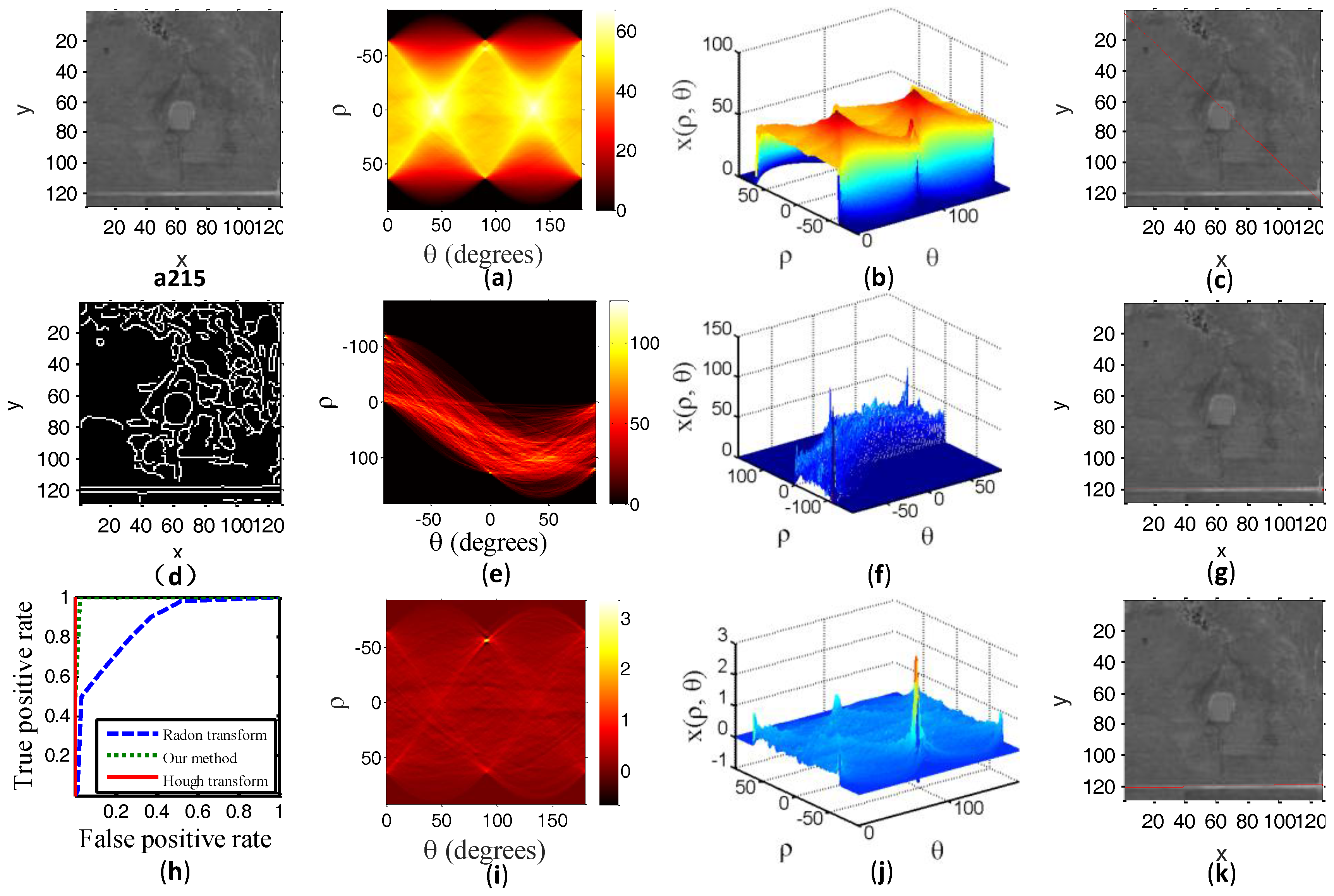
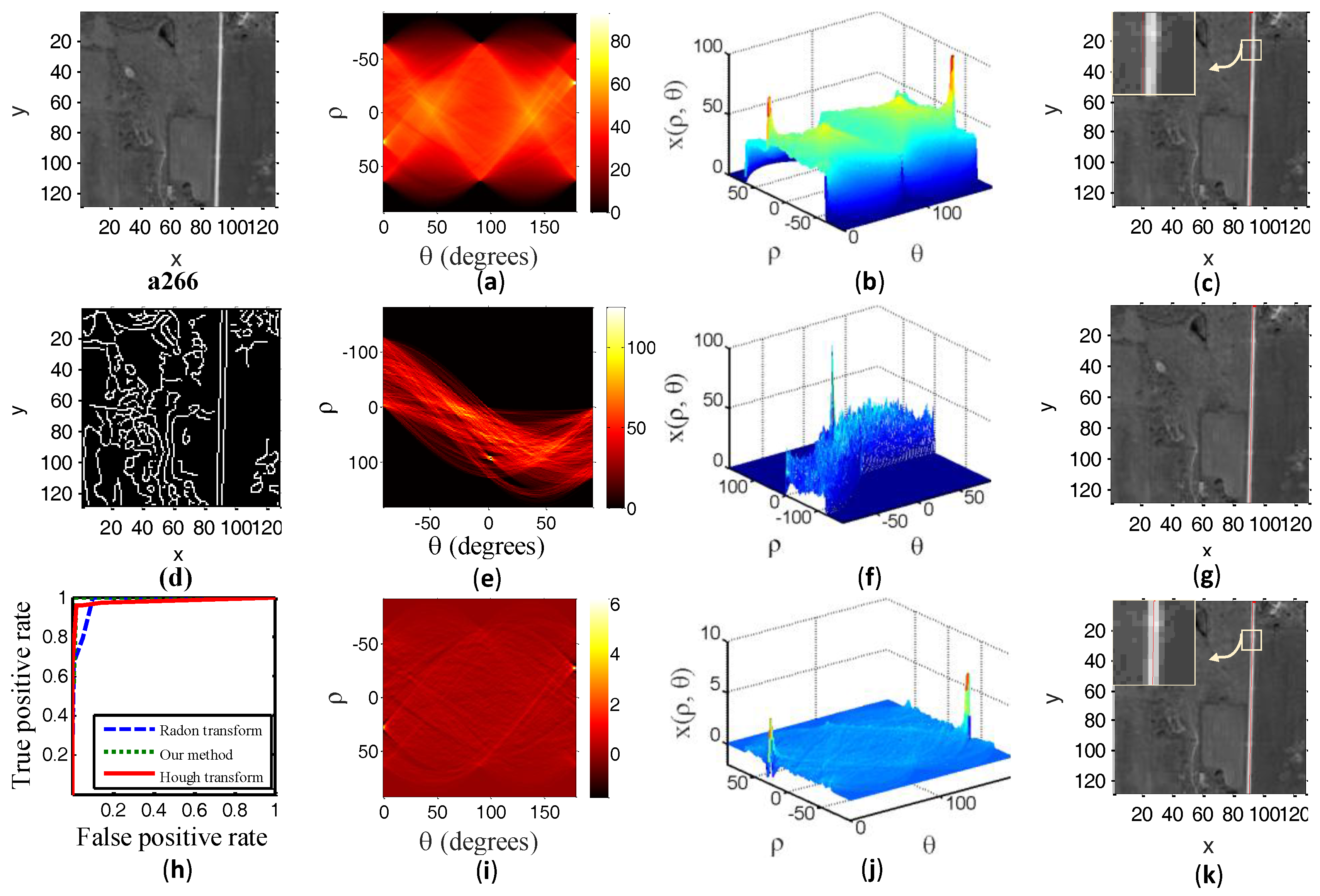
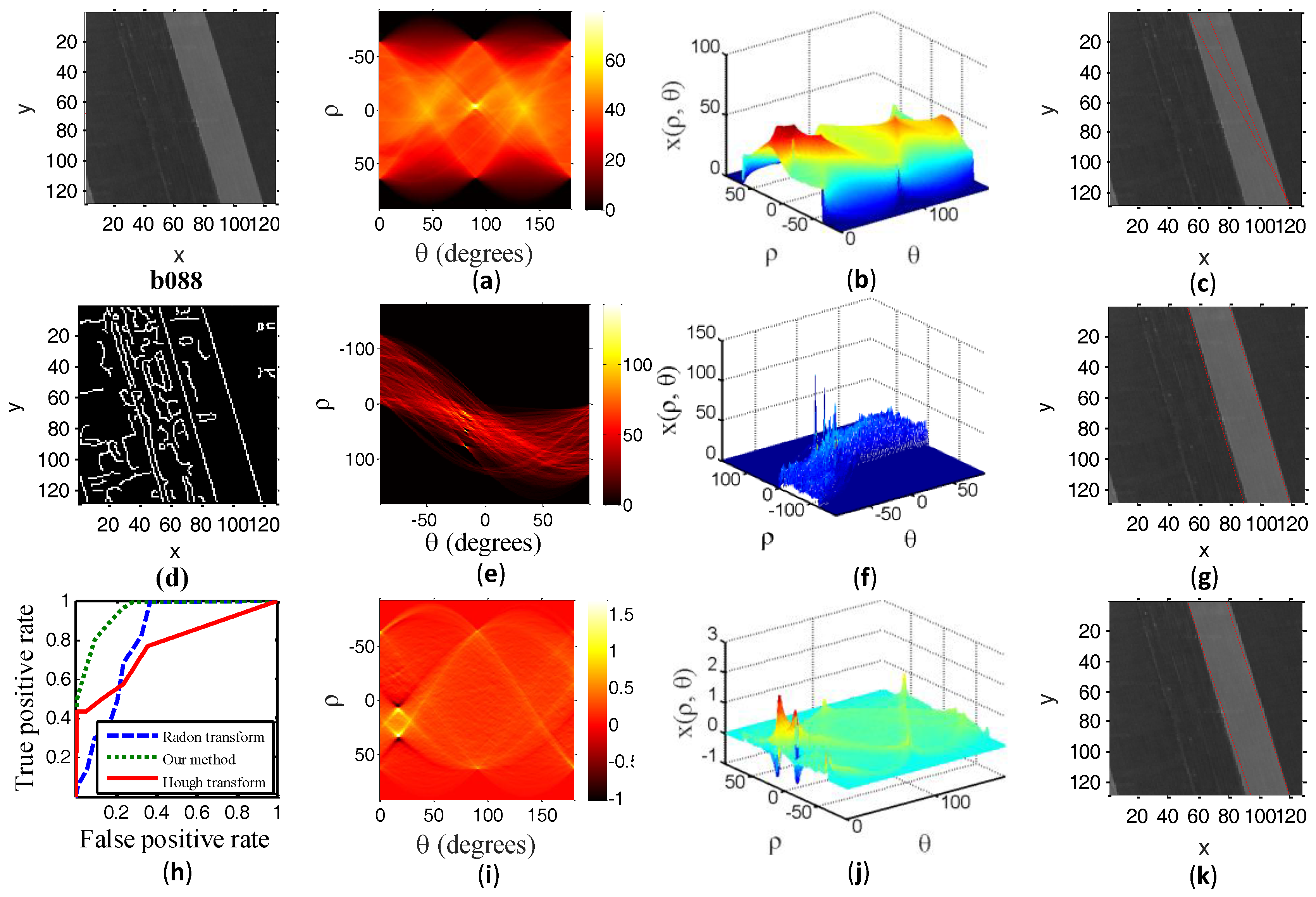
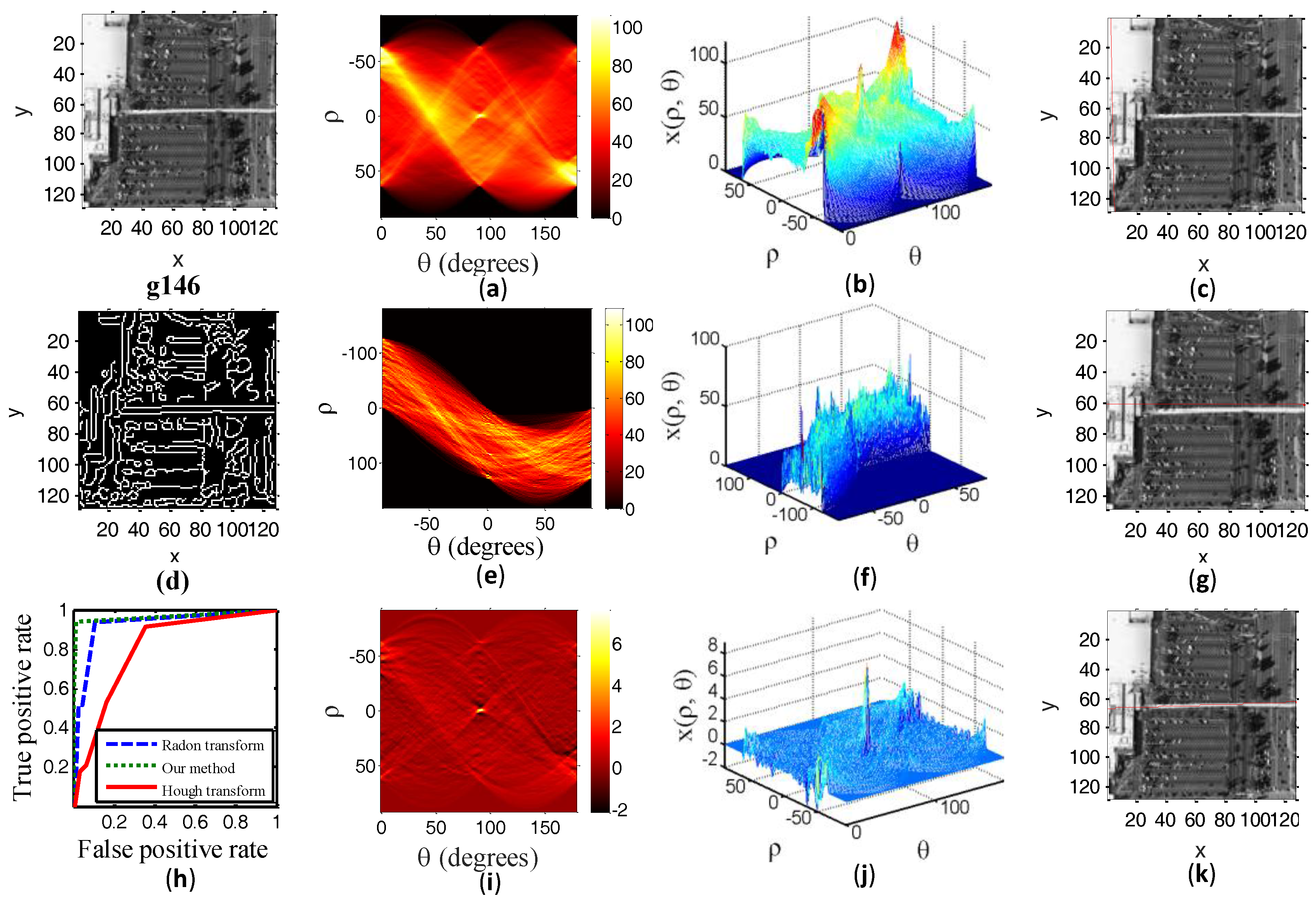
Figure 4a,
Figure 5a,
Figure 6a and
Figure 7a show the Radon transform of a test sample in a two-dimensional parameter space and
Figure 4i,
Figure 5i,
Figure 6i and
Figure 7i show the transform image from our method in a two-dimensional parameter space. The one distinctly bright spot in
Figure 4a,
Figure 5a,
Figure 6a and
Figure 7a and
Figure 4i,
Figure 5i,
Figure 6i and
Figure 7i corresponds to the detected line (i.e., a red line) overlaid on the test image. It cannot be easy to isolate this one distinctly bright spot which matches with the straight road in test images from transform domain due to a lot of interference highlights in
Figure 4a,
Figure 5a,
Figure 6a and
Figure 7a. However,
Figure 4i,
Figure 5i,
Figure 6i and
Figure 7i show a bright spot corresponding to the detected line overlaid on the test image. The bright spot area in
Figure 4a,
Figure 5a,
Figure 6a and
Figure 7a is cluttered in visual effect. However, our algorithm reduces the effect of cluttered interference bright spots. By comparing
Figure 4a,
Figure 5a,
Figure 6a and
Figure 7a with
Figure 4i,
Figure 5i,
Figure 6i and
Figure 7i, we can see that the proposed method is superior to the conventional Radon transform in terms of the visual effect.
Figure 4b,
Figure 5b,
Figure 6b and
Figure 7b show the three-dimensional form of Radon transform and
Figure 4j,
Figure 5j,
Figure 6j and
Figure 7j show the three-dimensional form of our method. The peak (i.e., bright spot in
Figure 4a,
Figure 5a,
Figure 6a and
Figure 7a) in
Figure 4b,
Figure 5b,
Figure 6b and
Figure 7b and
Figure 4j,
Figure 5j,
Figure 6j and
Figure 7j corresponds to the detected line overlaid on the test image. As seen in
Figure 4b,
Figure 5b,
Figure 6b and
Figure 7b, it cannot be easy to isolate the actual peak corresponding to the road in the test image from test samples owing to the mess in the transform domain. Particularly, the clutter of the peak in the transform domain will lead to false road detection or missed detection. From
Figure 4j,
Figure 5j,
Figure 6j and
Figure 7j, we can see that our method greatly accentuates the peak amplitudes relative to the background and it is possible to visually distinguish the peak point corresponding to the actual location of the straight road.
Figure 4j,
Figure 5j,
Figure 6j and
Figure 7j show that our method reduces the clutter interference to a large extent, and we are very easily able to isolate the true peak corresponding to the road in the test image.
Figure 4c,
Figure 5c,
Figure 6c and
Figure 7c show the detected line from our method overlaid on the test samples and
Figure 4k,
Figure 5k,
Figure 6k and
Figure 7k show the detected line from Radon transform overlaid on the test samples. The location of the true and estimated straight line road are shown in
Table 1. The ground truth parameters
of the straight road are obtained by manual marking in sample images.
It can be seen from the
Figure 4b,c that the peak point does not match with the straight road in test sample a215.
Figure 4j,k of test sample a215 show a conspicuous peak point which corresponds to the straight road in test sample a215. The experimental results of the test sample a215 illustrate that our method has a better detected result than traditional Radon transform if the detection target is not obvious.
The enlarged part in the
Figure 5c shows the detected line from Radon transform. The enlarged part in the
Figure 5k shows the detected line from our method. We can see that our detected results are closer to the true straight road.
By observing the
Figure 6b, we can see that the peaks in a three-dimensional parameter space do not focus on one point. Scattered peaks result in a wrong detection, while
Figure 6j illustrates that the peak point obtained by our method is more concentrated and easier to distinguish. From
Figure 6k, we can see that the detected lines from our method correspond to the actual location of roads.
Test sample g146 has some noises which are similar to the straight road. From
Figure 7c, we see that the detected line from the traditional Radon transform does not match with the straight road in the noisy image very well, whereas our method has good robustness for noisy images, as is shown in
Figure 7k.
The above experimental results indicate that our method can accurately detect the position of the straight road when the noise is high or the road characteristics are not obvious, which illustrates that our method has stronger robustness, and our detected results are closer to the actual road location.
We also compared our method with a traditional Hough transform. A Hough transform can only be used for binary images. Although the binary images weaken the background noise, they also cause the loss of some road information.
Figure 4d,
Figure 5d,
Figure 6d and
Figure 7d are the binary images of the test samples. By comparing the images of two-dimensional parameter space in
Figure 4,
Figure 5,
Figure 6 and
Figure 7, we see that
Figure 4e,
Figure 5e,
Figure 6e and
Figure 7e also have many interference bright spots although the binary image weakens the background noise. However,
Figure 4i,
Figure 5i,
Figure 6i and
Figure 7i only include true bright spots. From the transform images of three-dimensional form in
Figure 4,
Figure 5,
Figure 6 and
Figure 7, we see that our method greatly accentuates an area of high intensity in the transform domain relative to the background.
A binary image causes the loss of some road information. It can be seen from the
Figure 7g,k that the detected line from Hough transform does not correspond to the true position of the straight road.
To clearly compare our method with the Radon transform and Hough transform, we also report the Receiver Operator Curves (ROC) result in
Figure 4h,
Figure 5h,
Figure 6h and
Figure 7h. The ROC was produced by changing the threshold parameter. Specifically, we first determine a threshold parameter, if peak points surpass the threshold, it was classified as road pixels, or otherwise as noise pixels. The ground truth data was obtained by manual marking in remote sensing image. The
x-axis is the false positive rate (FPR) which can be calculated by:
the
y-axis is the true positive rate (TPR) which can be calculated by:
The accuracy of detected methods is measured through the area under the ROC curve. As shown in
Figure 4h,
Figure 5h,
Figure 6h and
Figure 7h, we can see that the accuracy of our method outperforms the traditional Radon transform and Hough transform.
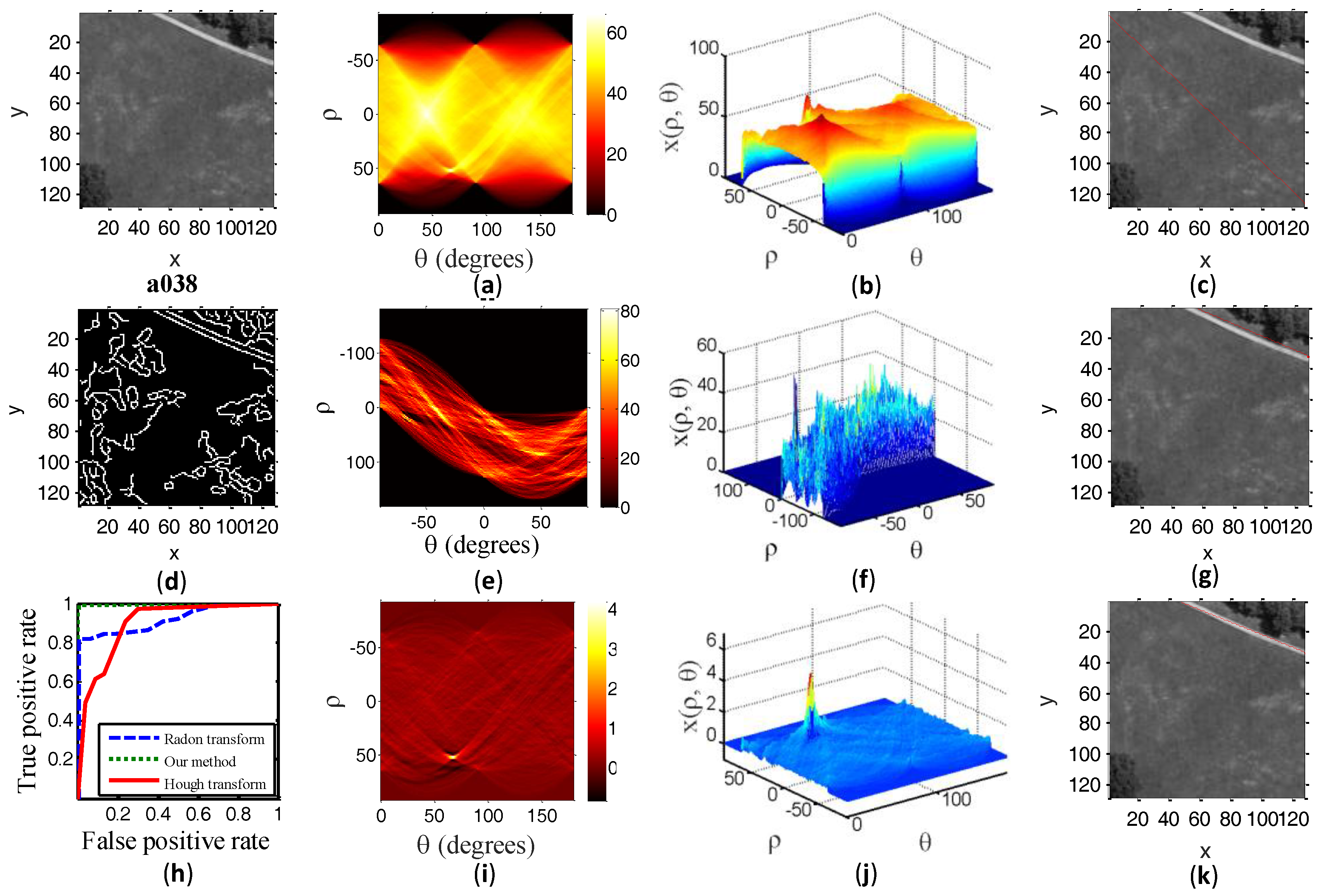
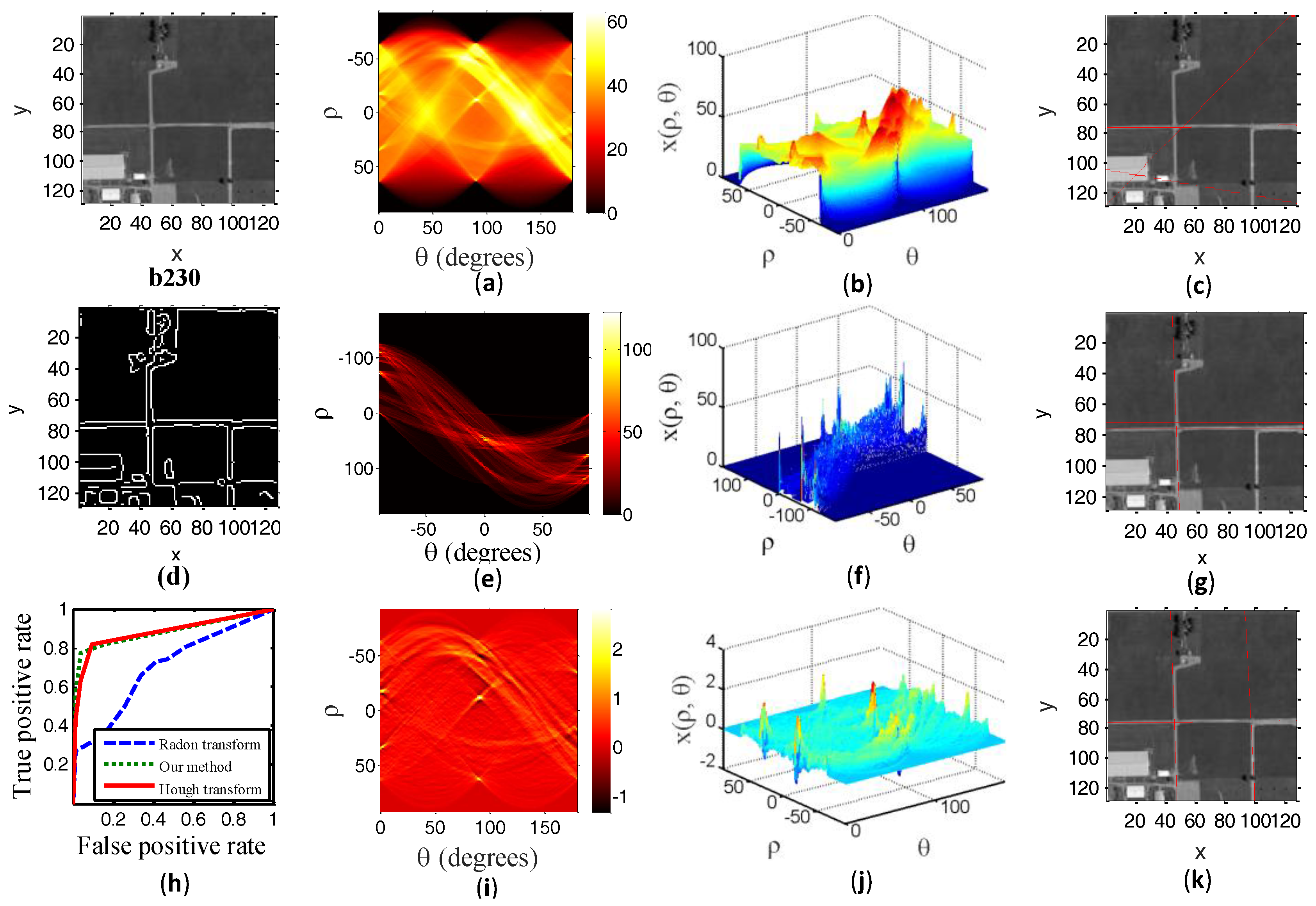
To further demonstrate the performance of our method, we show the experimental results of another two test samples in
Figure 8 and
Figure 9. The description of the experimental results in
Figure 8 and
Figure 9 is the same as above.
Specifically, test sample a038 shows a grayscale image with a shorter straight road.
Figure 8b shows an undistinguishable peak point due to the mess in transform domain, and the detected line overlaid on a038 does not match with the straight road. From
Figure 8j, we see that our method greatly accentuates an area of high intensity in the transform domain relative to the background. The experimental results in
Figure 8 illustrate that our method can well detect a shorter straight road. The same conclusion can be drawn in the experimental result of test sample b230. This indicates that our algorithm is more sensitive to a shorter line road.
Particularly, our method is able to complete the line road detection of multiple images at one time. In dealing with a large number of images, our method facilitates parallel implementation of the Radon transform for multiple images (i.e., replace vector
with a matrix).
Table 2 shows the time-consuming comparison between our method and the traditional Radon transform. We record the average running time of 20 test samples. Radon transform takes 0.106 s for per test image, but our method only takes 0.027 s. Experimental results of
Table 2 show that the computation of our method is nearly 4 times faster than Radon transform.
Above all, our method is superior to the traditional Radon transform in terms of accuracy and computing complexity.
Table 3 illustrates the mean-error and variance of error. We can see that the mean-error of our method is much lower than traditional Radon transform. Hence, the detected parameters
using our method is closer to the ground truth parameters. From the values of variance, we see that our method is more stable in detecting straight line.


