3.1. METRIC Evapotranspiration
METRIC is a satellite imagery-based processing model for estimating ET as a residual of the surface energy balance Equation (1) at the earth’s surface and is expressed as the energy consumed for evaporation.
where LE = latent energy consumed by ET (W/m
2), R
n = net radiation (W/m
2), G = soil heat flux (W/m
2), and H = sensible heat flux (W/m
2). We briefly summarize the components of the surface energy balance and ET calculation by METRIC below. More details on the METRIC ET estimation procedure are available from [
23,
24].
R
n represents all incident and reflected short and long wave fluxes and long wave radiant flux emitted from the surface (Equation (2)) and it is computed by subtracting all outgoing radiant fluxes from all incoming radiant fluxes [
23,
24].
where RS
i and RL
i are incoming shortwave radiation and incoming longwave radiation, respectively. RL
o is outgoing longwave radiation. The surface albedo (α) represents the surface reflectance characteristics and is the ratio of incident radiant flux to reflected radiant flux over the solar spectrum, and ε
o is the broadband surface emissivity.
G is the rate of soil heat flux due to conduction, and is calculated using an empirical equation developed by [
33] as:
where LAI is the leaf area index (unitless) and is estimated as a function of SAVI (Soil Adjusted Vegetation Index), as described in [
34]. T
s is the surface temperature (Kelvin, K) and is estimated by using a modified Plank equation following [
35] with atmospheric and surface emissivity correction [
23].
H is the rate of heat flux to air by conduction and convection, and is computed as:
where ρ = air density (kg/m
3), c
p = air specific heat (J/kg/K), dT = the temperature difference between two heights (z1 and z2) in a near surface blended layer, and r
ah = aerodynamic resistance to heat transport (s/m) between heights z1 and z2.
The calibration of H is accomplished by inverting Equation (4) at two extreme ET conditions present within the image. These extreme ET conditions refer to the wettest and driest conditions and are represented by two anchor pixels, namely a cold pixel (high ET) and a hot pixel (zero or near-zero ET), selected within the image (more description in
Section 3.2). Its calibration is based on a linear relationship between the surface temperature (T
s) and dT at two anchor pixels. r
ah is estimated during an iterative process based on the friction velocity of the air, the momentum roughness length of the surface, and atmospheric stability [
18]. The hot pixel is usually selected from the bare soil surface with a lower Normalized Difference Vegetation Index (NDVI) (<0.20) and higher surface temperature, where the ET rate is assumed to be near zero. The cold pixel is selected from fully covered actively growing agricultural fields which have a lower surface temperature and a high NDVI (>0.75), representing a near potential ET rate [
23,
24,
28].
After computing R
n, G, and H, LE is computed as a residual of the surface energy balance by applying Equation (1). LE is divided by the latent heat of vaporization (λ) to compute instantaneous ET at the time of satellite overpass. Extrapolation of instantaneous ET (ET
inst) to 24-h (daily) ET is obtained by employing the reference ET fraction (ET
rF). ET
rF is synonymous with the well-known crop coefficient (Kc) and is computed as a ratio of ET
inst to instantaneous reference ET (ET
r inst) at the satellite overpass time. ET
r inst is calculated by employing local meteorological data, as detailed in ASCE-EWRI [
36]. The instantaneous ET
rF computed at the satellite over pass time is assumed to be equivalent to a 24-hour average [
23,
36]. The instantaneous ET
rF is then multiplied with daily ET
r to obtain the daily ET.
3.2. METRIC Application in the Southern Amazon
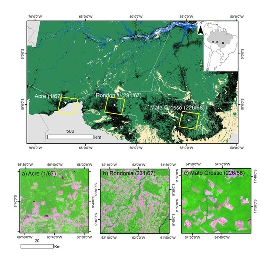
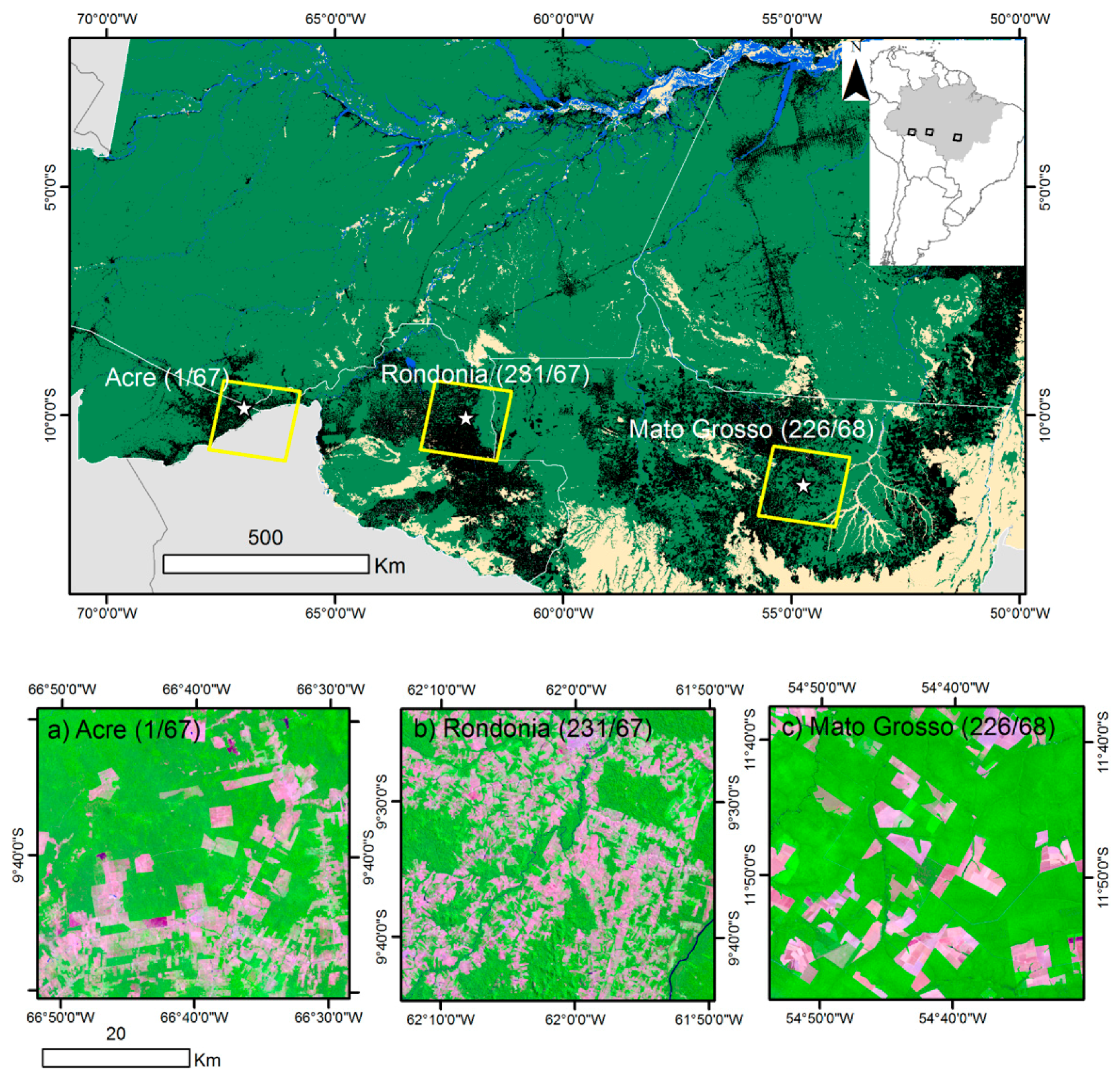
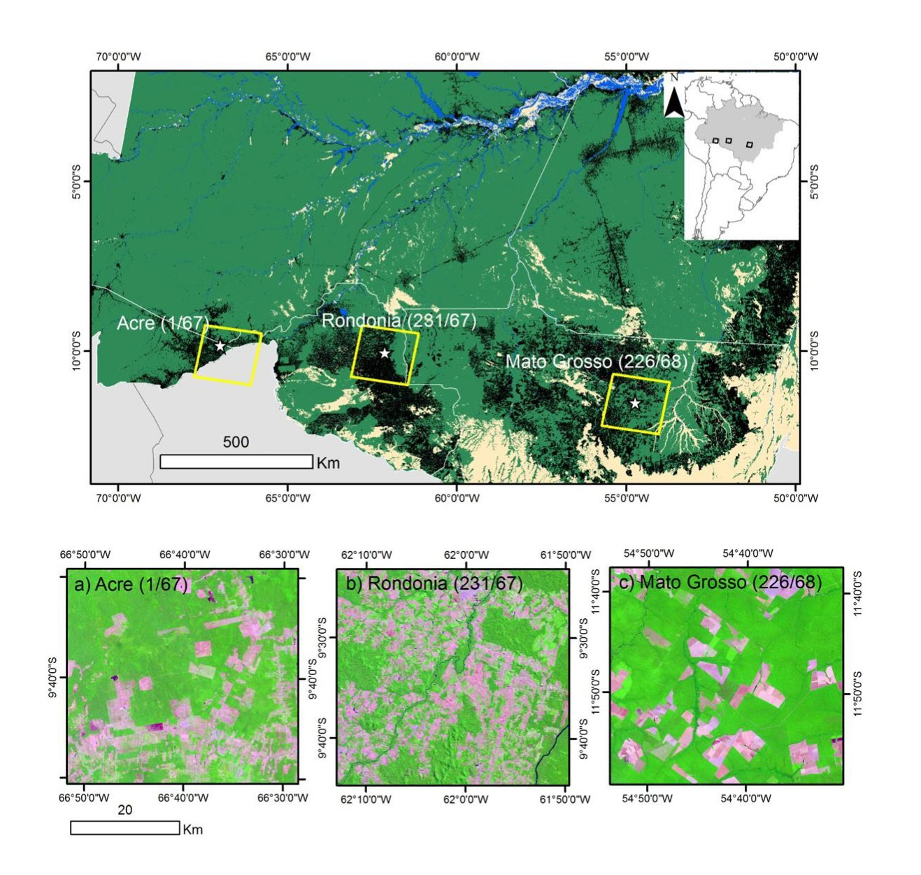
METRIC processing requires four primary inputs: Landsat imagery, local weather data, land cover maps, and Digital Elevation Model (DEM) maps. The Landsat images (
Table 3) for this study were downloaded from the USGS Global Visualization Viewer (
http://glovis.usgs.gov/). Hourly weather data were collected from weather stations/flux towers over pasture (
Table 1) and went through a rigorous quality control process [
36,
37] to ensure their integrity before computing reference ET (ET
r) and METRIC processing. Land cover maps developed by [
38] were used. Elevation maps based on NASA Shuttle Radar Topography Mission (SRTM) data (resampled to 30 m horizontal resolution) were used. Elevation maps were used to adjust the surface temperature and radiation flux as a function of elevation, and land cover maps [
38] were used for developing spatial variations in surface roughness.
METRIC utilizes the Calibration using Inverse Modeling at Extreme Conditions (CIMEC) procedure as used in the Surface Energy Balance Algorithm for Land (SEBAL) [
18,
39] to estimate the dT function (Equation (4)) for the computation of sensible heat flux. The estimation of dT is facilitated by selecting anchor pixels (cold and hot pixels) within the Landsat image. Ideally, cold pixels are selected from agricultural fields with green, actively growing vegetation cover representing the upper end of the ET spectrum within the image. However, in our study in the southwestern Amazon (Acre and Rondônia), pasture regions were considered the most appropriate land use for the selection of cold pixels due to the difficulty in finding suitable agricultural vegetated area [
28]. For consistency, cold pixels in Mato Grosso were also selected from fields with pasture even though there were some crop fields observed within the image. These crop fields were used to confirm the final calibration at the cold pixel. Hot pixels were selected from bare soil surface areas with very little vegetation (NDVI < 0.20) representing near zero ET unless residual soil evaporation from antecedent rainfall was present. A bare soil evaporation model [
40] was run on a daily time step to adjust for any residual soil evaporation. Additional detail about an iterative process of selecting the cold and hot pixels is described in [
28].
ET
rF at the cold pixel is typically assumed to be equivalent to 1.05 [
23]. Identifying green pasture for the cold pixel with NDVI > 0.75 during the dry season is challenging. Therefore, the NDVI values of those selected cold pixels were less than that of the ideal cold pixel (>0.75). For this lower NDVI situation, an alternative approach was used to adjust the ET
rF fraction for the cold pixel (Equation (5)) [
23,
40]. The NDVI-based approximation procedure in (Equation (5)) is commonly applied during non-growing seasons in agricultural settings when the crops are not fully developed, or when the ground is not fully covered by crops. This NDVI indexed approach has been tested during the dry seasons in Rondônia and showed a good agreement with the flux tower ET observations [
28].
During the first step (METRIC
1), we used an empirical equation from [
23] as a general approach for agricultural areas in the non-growing season as:
where NDVI
cold is the NDVI at the cold pixel. This procedure is termed METRIC
1 hereafter.
We also tested a procedure (Equation (6)) suggested by [
23] and applied by [
26] in the Middle Rio Grande of New Mexico which is based on local data and operator’s judgement, for each Landsat scene in our study region. In Equation (6) (henceforth termed METRIC
2), a linear equation between ET
rF and NDVI was developed at each Landsat sceneto generate new ET
rF
cold values for the cold pixels:
where
a and
b are empirically determined constants, the slope and intercept, for a given linear relationship between ET
rF
cold and NDVI
cold for each Landsat scene.
To calculate ET
rF
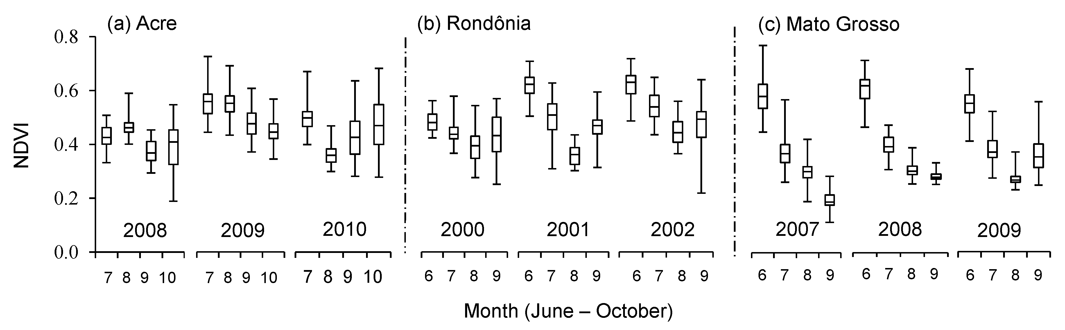
cold from these two approaches (Equations (5) and (6)), we first selected fifty 10 by 10-pixel sample polygons (300 m by 300 m) of NDVI from pasture areas at each one of the 36 Landsat images (
Table 3). Each sample was located no nearer to the pasture field edges than 90 m to avoid signal contamination within the thermal band during the subsequent processing. From these NDVI samples, the top 20% NDVI (10 samples) from each image was further selected as a representation of potential samples for the selection of the cold pixel. For the METRIC
1 procedure, a suitable cold pixel was selected from the top 20% NDVI samples for each image and Equation (4) was applied for complete METRIC processing. For the METRIC
2 approach, the ET
rF values (ET
rF
1) obtained from METRIC
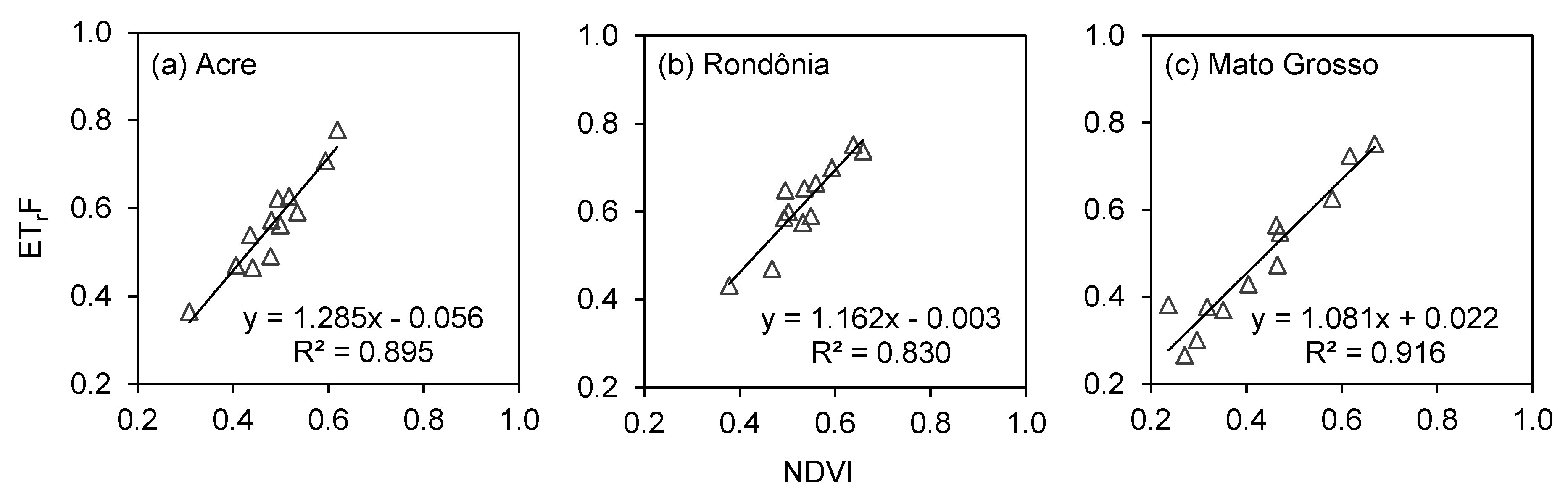
1 were integrated with the top 20% NDVI samples to develop linear regression equations at each Landsat scene. To generate this NDVI-ET
rF equation, the ET
rF
1 values corresponding to the top 20% NDVI samples were extracted and averaged for each image date (
Table 4). One image from each month was selected during the dry season months to cover the seasonal NDVI variations across the study sites. The linear relationship at each Landsat scene was developed using 12 data points (for 12 image dates). These new developed equations for each Landsat scene were applied for the complete processing of the METRIC
2 approach. While the cold pixel was the same for these two different METRIC approaches for the same image date, the ET
rF
cold values were different, depending on the equation used (Equations (5) and (6)). The unique set of cold and hot pixels was selected for each image date and iterative post-processing was completed until a suitable set of anchor pixels were identified.
For the application of METRIC in Amazonian forest, some adjustments were made such as improvements for the estimation of surface roughness length (zom) and surface temperature (T
s), as described in [
28]. To improve the zom estimation across multiple forest types, the zom estimation method by [
41] was used. The Perrier zom estimation is based on LAI, average tree height, and vertical canopy distribution. The zom values for multiple forest types such as primary forest, regenerated forest, and degraded forest (Mato Grosso only), were calculated. The heights of primary and regenerated forests were considered to be 30 m and 20 m, respectively, and degraded forests were 15 m. The canopy distribution was assumed to be uniform for primary and regenerated forests, and sparsely topped canopy for degraded forests. The maximum value of zom for each forest type was limited to 1.0 m. To account for the potential T
s reduction due to shadow impacts on albedo resulting from differences in the sun angle to that of the nadir-viewing satellite in tall vegetation, a linear adjustment on ET
rF based on the surface albedo, NDVI, T
s, and ET
rF of the hot and the cold pixels was made [
34]. However, due to a small impact of T
s adjustment (i.e., <2%) on the final forest ET, the standard method of T
s estimation within the METRIC procedure was followed in this study.
3.3. Comparison to Flux-Tower ET Estimates
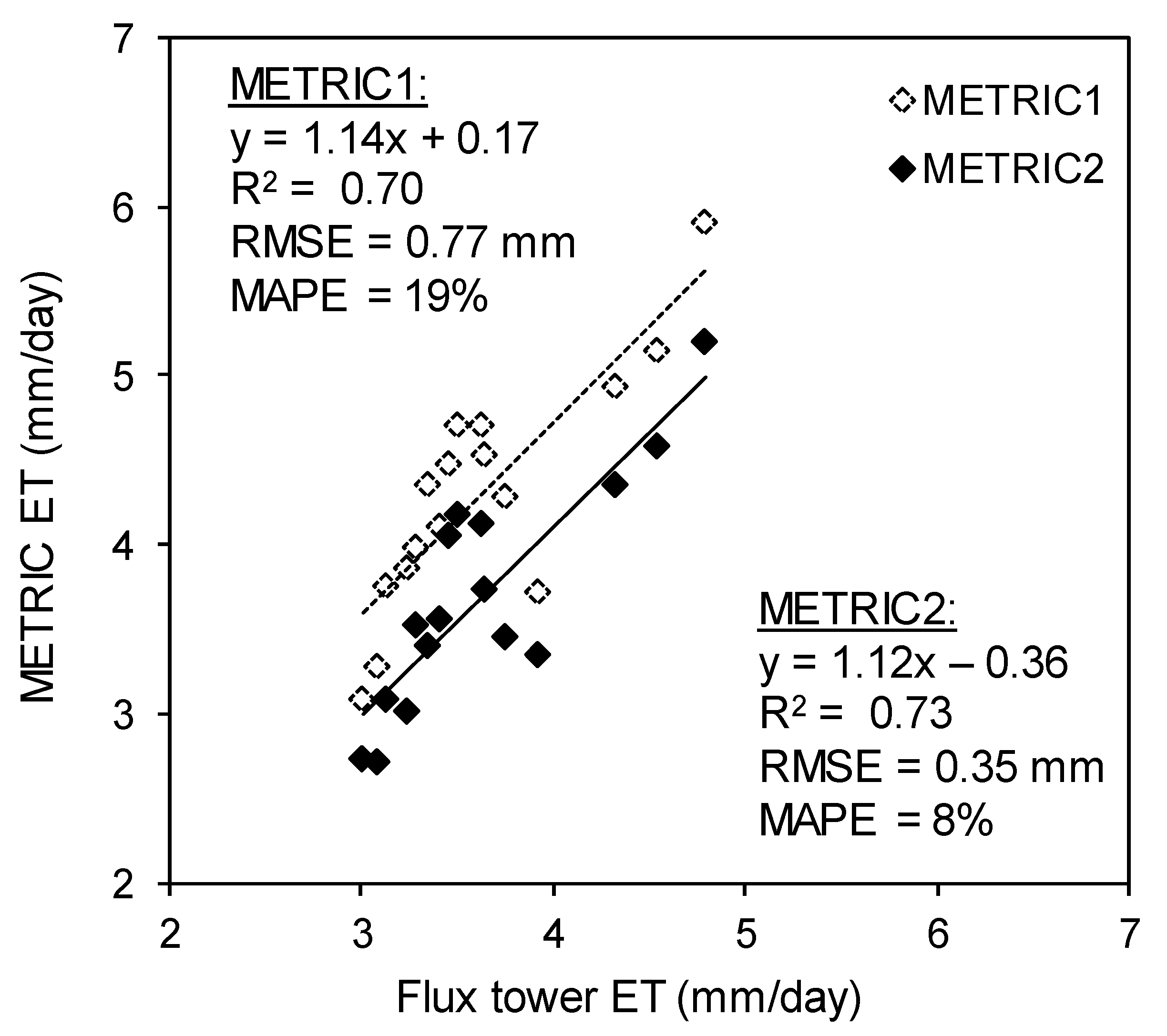
Daily forest ET data from the METRIC procedure (METRIC
1 and METRIC
2) were compared to flux tower ET data. A common challenge with flux tower ET is the lack of energy balance closure [
42,
43]; therefore, comparisons were only made with the energy balance closure (EBC) ratio (H + LE)/(R
n − G)) ≥0.80. In other words, METRIC and flux tower ET were only compared on days with an EBC error of less than 20%. For the comparable image days, energy balance closure errors (R
n − H − LE − G) in flux tower data were distributed between H and LE by applying the constant Bowen-ratio approach [
42] to compute the daily ET from the flux tower. ET data from METRIC were extracted by taking three different pixel window sizes (3 × 3, 5 × 5, and 9 × 9) centered on the flux tower location to identify the appropriate sampling area. The ET comparisons showed less (within 0.2 mm/day) variation among these sampling units, indicating homogeneous land covers around the flux towers; therefore, 3 × 3 pixel window was chosen for comparisons and analysis [
28].
The errors and accuracy estimation between the METRIC procedures (METRIC
1 and METRIC
2) and flux tower ET were made by computing the root mean square error (RMSE) and mean absolute percentage error (MAPE) as:
where METRIC ET is the ET estimated from METRIC and flux-tower ET from flux tower observations, and n is the number of days available for comparison. The agreement between the daily flux-tower ET and METRIC ET was tested by the coefficient of determination (R
2) of a linear regression line.
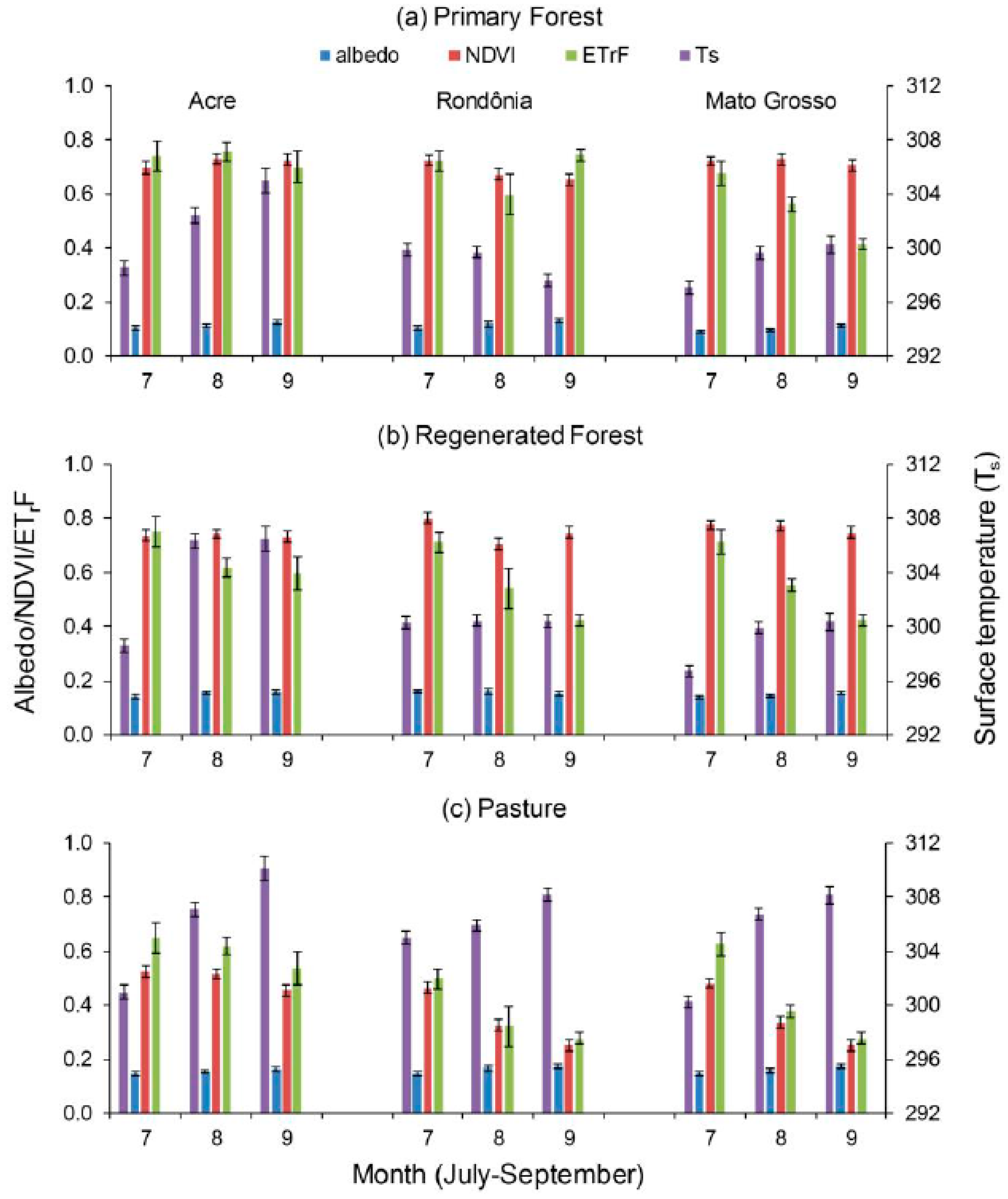
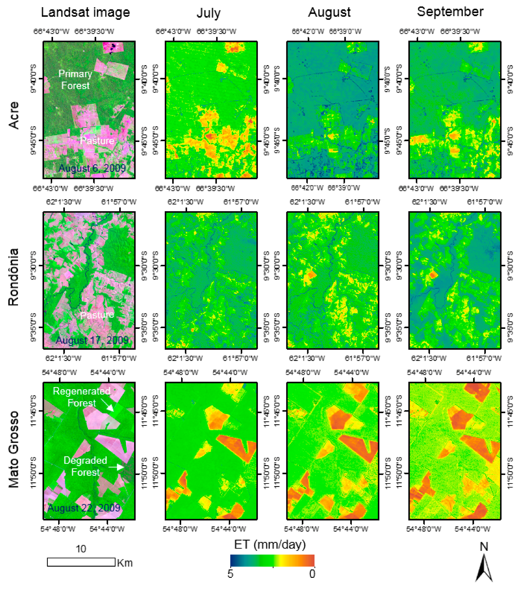
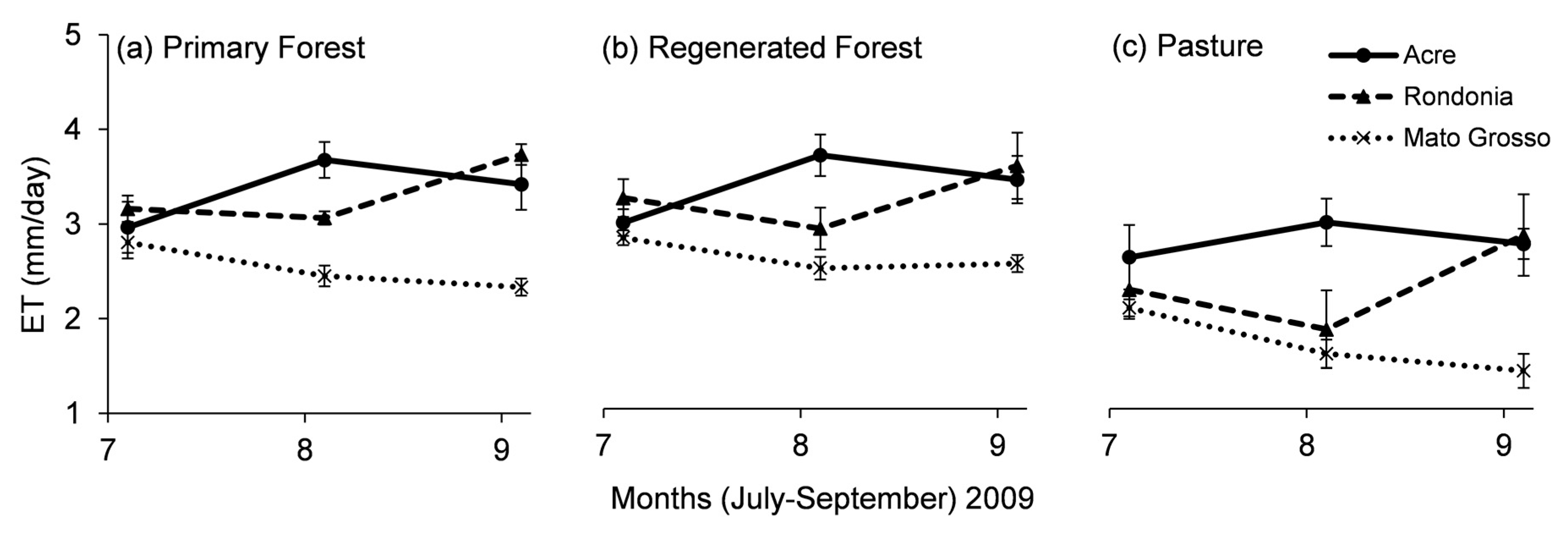
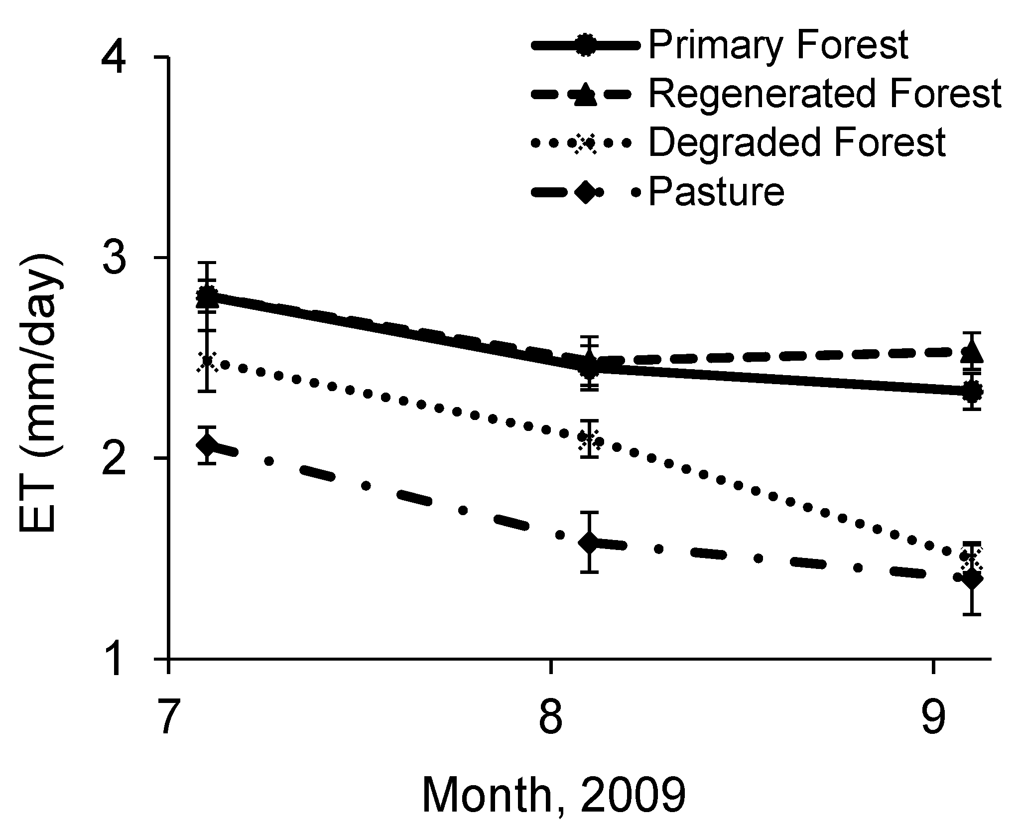
3.4. Characterization of Dry Season ET Patterns from Different Land Cover Types in the Southern Amazon
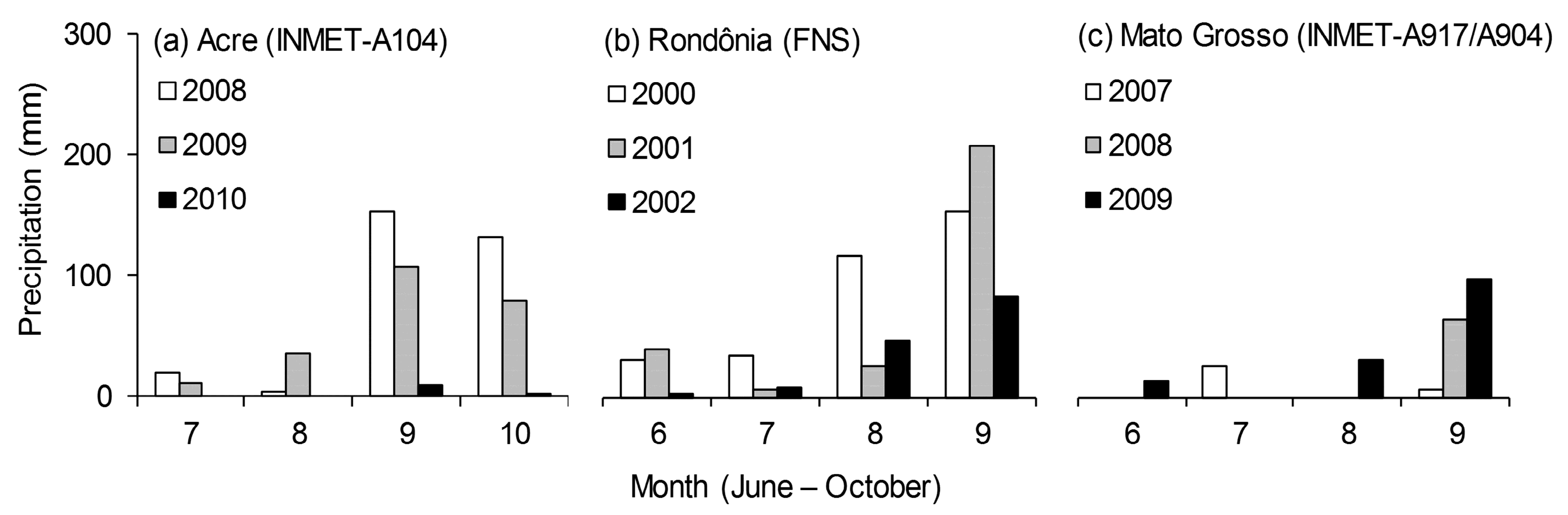
The METRIC2 approach was applied to estimate ET from different land cover types including intact forest, regeneration, degraded (burned forest) forest, and pasture to characterize their variation during the dry season of the year 2009 across three study sites as a further improvement of the NDVI-indexed ET estimation. Dry seasons at the study sites usually last for three to five months; however, the dry season ET comparison and analysis were made from July to September to be consistent with the time period across all study sites. Daily ET estimates were obtained as a product of daily ETrF2 (from EMTRIC2) and corresponding ETr. The ETrF2 values between the satellite overpass dates were obtained by spline interpolation. The average monthly ET was computed as a simple division of the monthly ET (sum of daily ET) by the number of days for the specific month. The average monthly ET rates from each land cover type were computed by taking averaged values of 10 samples from each land cover type within a Landsat scene. Each sample was 10 by 10 pixels and selected so as to cover the spatial distribution of each land cover type within an image.
Identification of primary forest, regenerated forest, degraded forest (only in Mato Grosso), and pasture land cover types within a satellite image was made with references from the land cover products “TerraClass” [
44] and forest degradation products by the Brazil’s National Institute for Space Research (INPE-DEGRAD) [
31]. The INPE TerraClass is available for 2008, 2010, and 2012 as of the time of our analysis (
http://www.inpe.br/cra/ingles/project_research/terraclass.php). To confirm the same land cover type for our study year 2009, we considered the TerraClass products of the years 2008 and 2010. For degraded forest (burned forests) in Mato Grosso, INPE DEGRAD data (INPE, 2016) was used for 2009.
Statistical analyses of dry season ET from different land covers were made by applying one-way analysis of variance (ANOVA) and student’s t-test at the 5% significance level.


