3.1. Dataset
Targeting the classification of tactile data, the use of the dataset collected in [
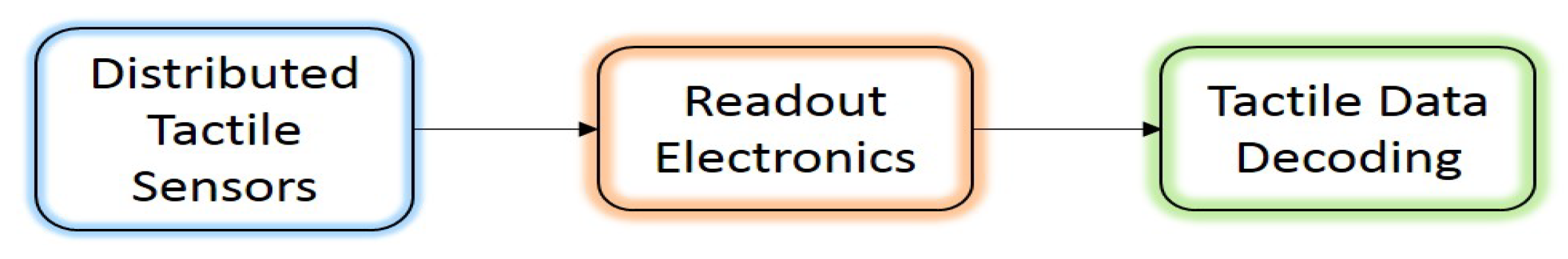
5] was considered. Tactile data were collected by a high resolution (1400 pressure taxels) tactile array, which was attached to the 6 DOF robotic arm AUBO Our-i5 [
5]. A set of piezoresistive tactile sensors was distributed with a density of 27.6 taxels/cm
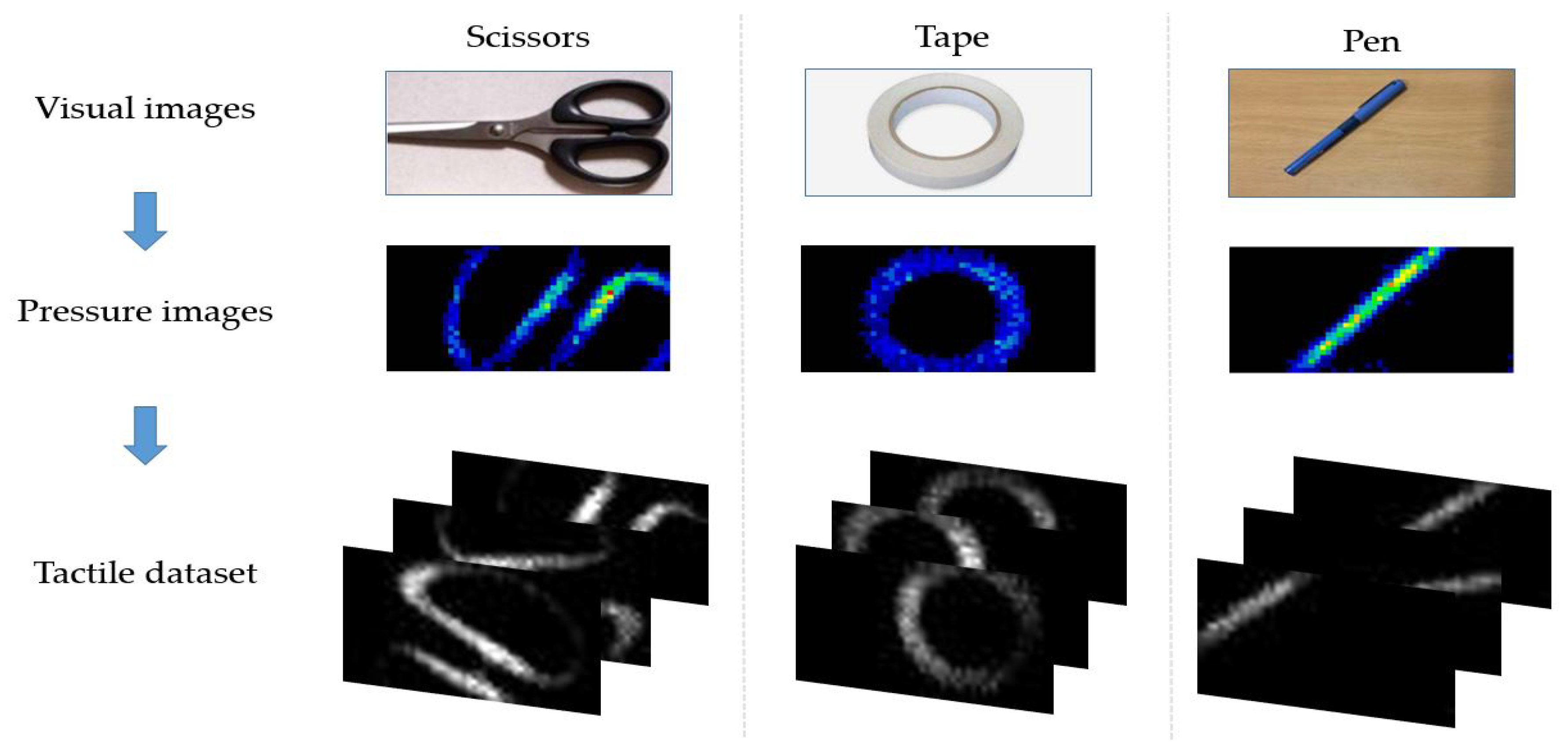
, forming a matrix of 28 rows by 50 columns. The dataset was composed of pressure images that presented the compliance of 22 objects with the tactile sensors. These images were divided into 22 classes labeled as adhesive, Allen key, arm, ball, bottle, box, branch, cable, cable pipe, caliper, can, finger, hand, highlighter pen, key, pen, pliers, rock, rubber, scissors, sticky tape, and tube.
Figure 2 shows an example of the tactile images of three objects used for the training of the CNN model. Each taxel in the tactile array presents a pixel in the pressure image; thus, each pressure image is 28 × 50 × 3 in size. Therefore, the color of the pixel presents the pressure applied at the corresponding taxel. The minimum pressure is presented by black color, and the maximum pressure is presented by red color. Pressure images were then transformed into grayscale images (image size = 28 × 50 × 1), forming the tactile dataset.
3.2. Tested Model
Due to computational and memory limitations in the embedded application, a light CNN model was required to perform classification tasks with high accuracy and fewer parameters. In this work, we chose to use one of the models implemented in [
5] as a base model to classify the objects in the aforementioned dataset. Among all the implemented networks, we chose to use the custom network TacNet4 because it was the best network that fit the embedded application (fewer parameters with high accuracy [
5]). The model was based on AlexNet, which is usually used in computer vision for object classification [
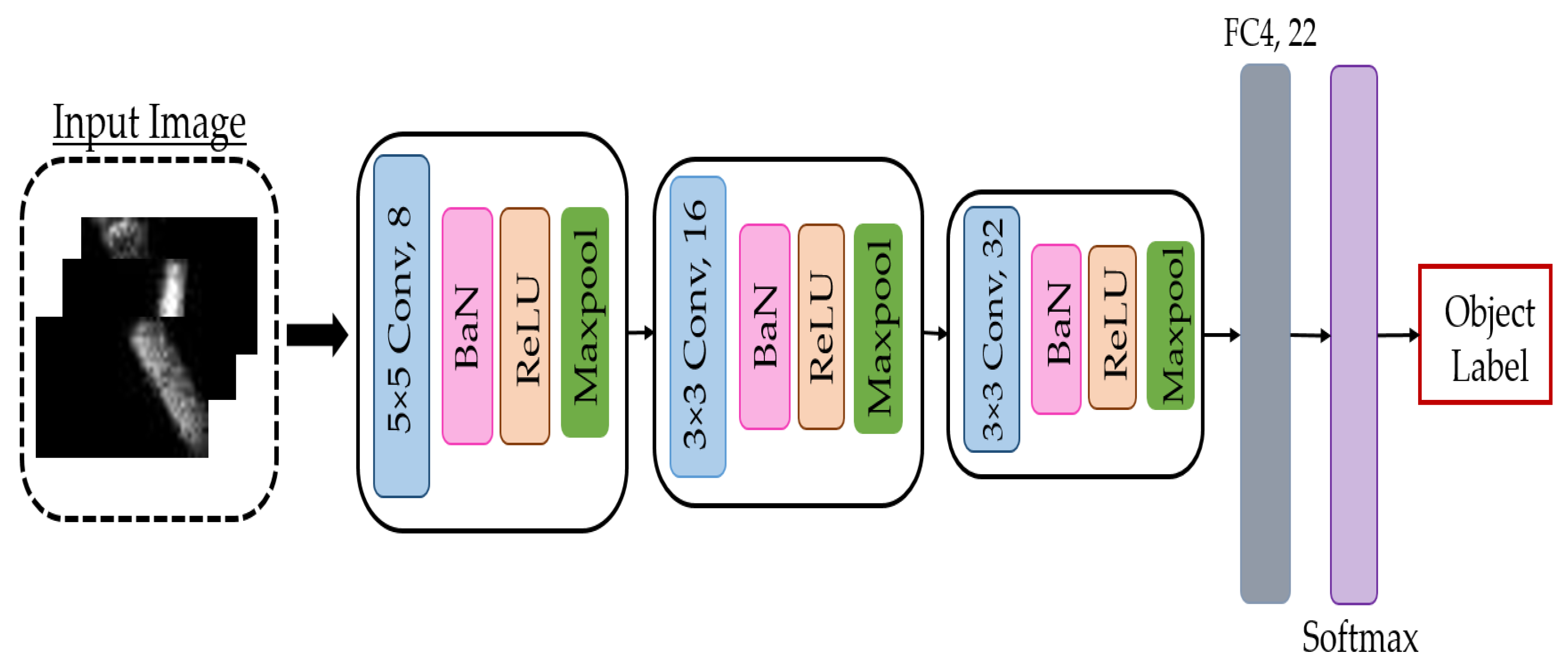
23]. The network was composed of 3 Convolutional layers (Conv1, Conv2, and Conv3) with filters sizes (5 × 5, 8), (3 × 3, 16), and (3 × 3, 32) respectively. Each convolutional layer was followed by a Batch Normalization (BaN), Activation (ReLU), and Maxpooling (Maxpool) layer, respectively, where all pooling layers used 2 × 2 maxpooling with a stride of two. A Fully Connected layer (FC = [fc4]) with 22 neurons followed by a softmax layer were used to classify the input tactile data and give the likelihood of belonging to each class (object). The input shape of the model was configured to the size of the collected tactile data.
Figure 3 shows the detailed structure of the network used.
The network was implemented in MATLAB R2019b using the Neural Network Toolbox. A total of 1100 tactile images were used to train the model. The learning process was implemented in MATLAB by dividing the tactile data into three sets: training, validation, and test sets.
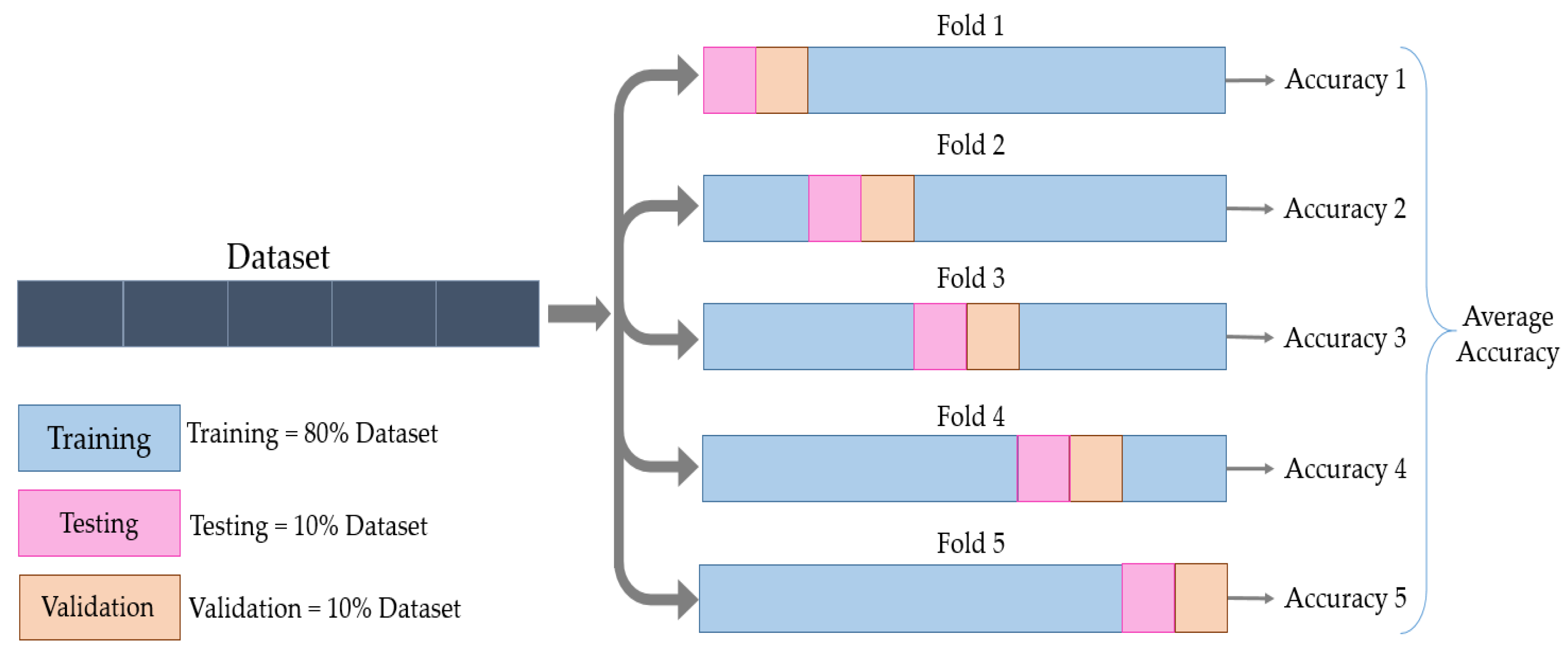
When having an adequate dataset, the validation set is expected to be a good statistical representation of the entire dataset. If not, the results of the training procedure highly depend on how the dataset is divided.
To avoid this, In this work, we used the cross-validation method. The data were partitioned into five folds, and each fold was divided into training, validation, and test sets. The training set formed 80% of the dataset, and the validation and test sets formed 10% each. This process was then repeated five times until all the folds were used, without having common elements across all folds for the validation and test sets, as shown in
Figure 4.
For each training process, the training set was composed of 880 images, 40 images for each label, whilst each of the validation and test sets was composed of 110 images. Training the model from scratch required a large dataset to achieve high accuracy. For that reason, data augmentation techniques, i.e., flipping, rotation, and translation in the X and Y axis, were applied to the dataset. Hence, the amount of tactile data available for training and validation was increased to 5280 and 660, respectively. The performance of the implemented model was evaluated based on the recognition rates achieved in a classification experiment of the test set composed of 110 original images (objects) from 22 classes.
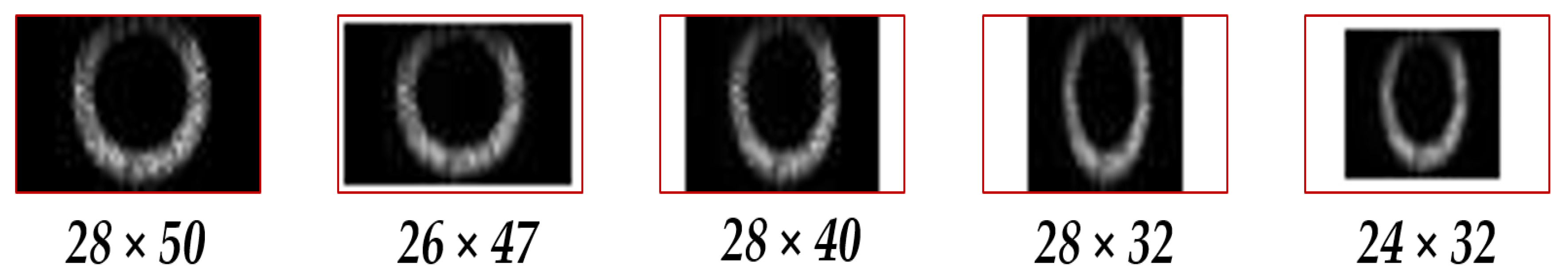
For embedded applications, with computational, memory, and energy constraints, it is necessary to decrease the number of trainable parameters in the CNN model. In this work, we chose to decrease the number of parameters of the trained model by decreasing the input image size (i.e., lower resolution images); an example is shown in
Figure 5. For that reason, several experiments were performed to choose the smaller size of the input data, keeping the same classification accuracy. The input shapes were chosen in a way that each shape resulted in a reduction of the number of parameters.
Table 1 shows how the number of parameters of the layers depended on the input shape. The change in the input shape affected only the number of parameters of the fully connected layer. This was due to the fact that the number of parameters in the convolutional layer depended only on the size and number of the filters assigned for each layer (((width of the filter × height of the filter) + 1) × No. of filters), while in the FC layer, the number of parameters ((No. of neurons in the FC layer × No. of neurons in the previous layer) + 1) was affected by the size of the input image and the output layer. The performance of the model was studied with five different input shapes, as shown in
Table 1. This resulted in five different models with different input shapes, each one trained from scratch 5 times (one time per fold), which output 25 trained NNs.
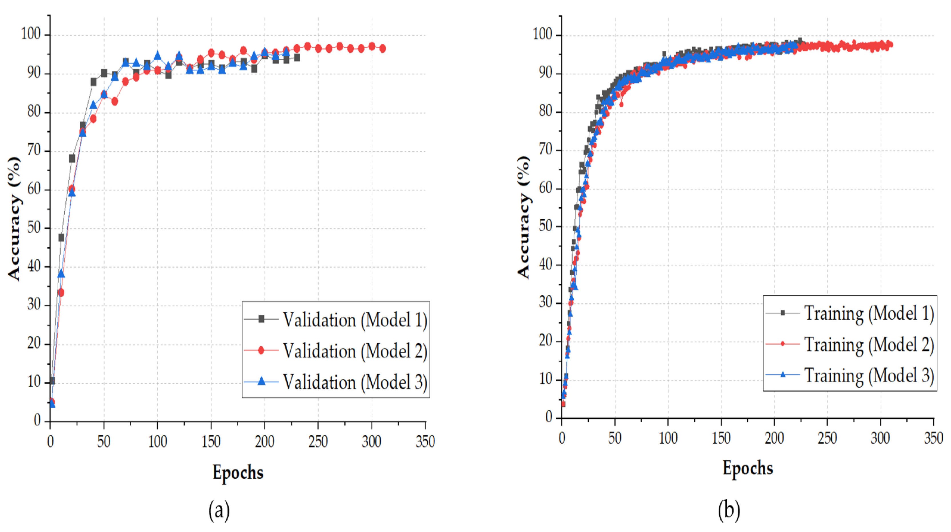
Figure 6 shows the training and validation accuracy over epochs, for the first three models among the five models. The figure shows that the accuracy achieved by the three models was close to 100%. Each model was evaluated with MATLAB by running a classification task on the test set.
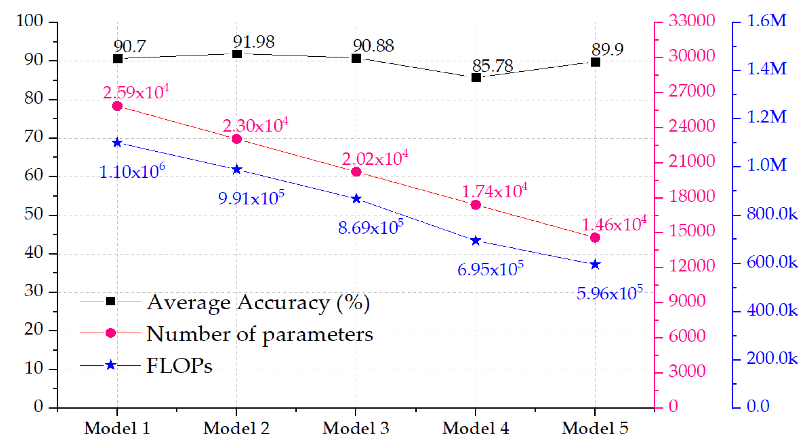
Figure 7 shows the change in the number of trainable parameters and the average classification accuracy, with respect to the change in the input shape, as well as the FLOPs. The classification accuracy presented the average test accuracy among the five folds. The figure shows that it was possible to decrease the input size from 28 × 50 × 1 to 26 × 47 × 1 or to 28 × 40 × 1 and achieve an increase in the classification accuracy from 90.70% to 91.98% and 90.88%, respectively. Decreasing the input size of the model resulted in a drop in the trainable parameters from 25,862 to 23,046 and 20,230 parameters, respectively, for the aforementioned models. This decrease in the number of parameters would also induce a decrease of the number of Floating Point Operations (FLOPs), as shown in
Figure 7; the average ratio of the decrease in the number of parameters with respect to the decrease in the number of FLOPs was 1/44 i.e., with each decrease in number of parameters, there was a 44 times decrease of the FLOPs. The number of FLOPS in
Figure 7 corresponds to the convolutional layers only, where most of the FLOPs were, and these FLOPs were calculated according to the following formula [
24]: FLOPs = n × m × k, where n is the number of kernels, k is the size of the kernel (width × height × depth), and m the size of output feature map (width × height), while the depth in the kernel size corresponds to the depth of the input feature map.


