The shape of the solder joint has a significant effect on the interface contact pressure, and a small size fluctuation will change the maximum contact pressure value at the interface of the solder joints, which will affect the interface crack initiation earlier or the expansion of the solder joint to generate a larger crack, which will ultimately lead to the failure of the solder joint. The objective of this section is not to limit the contact pressure at the critical points but to shift to the average contact pressure values in the zones prone to interface delamination (as analyzed in
Section 2). This not only reduces the contact pressure of the interface critical points, making it not easy to delaminate but also reduces the contact pressure of the nearby area, which can reduce the risk of further crack propagation even if cracks occur in the solder joint.
4.1. A Brief Review: Kriging Surrogate Model and EGO Method
Th Kriging surrogate model (which is more commonly called the Gaussian process in the emerging field of artificial intelligence) is a high-precision interpolated response surface model that uses the sum of regression functions and random processes to represent the functional relationship between design variables and response variables [
31]. The biggest difference between the Kriging surrogate and the traditional polynomial response surface model is that it uses statistical assumptions to interpret the results of the surrogate model. The expression of the Kriging model is:
where,
is the basic function of the Kriging surrogate, and the polynomial basis function is generally used.
is the regression coefficient;
represents the expectation of random function
;
is a static random process with a mean of 0 and a variance of
. Physically speaking, the first term
roughly represents the overall trend of the model, giving the general position of the real model at the prediction point. The second term
represents the spatial correlation of the relevant parameters in the design space, giving the local deviation of the model at the prediction point.
It is worth emphasizing that, compared with other surrogate models, such as polynomial response surface, Kriging can not only provide the prediction response but also provide the uncertainty of the prediction. This property can be very useful for adaptive optimization. Jones et al. proposed the Efficient Global Optimization (EGO) algorithm, which uses a so-called adaptive learning function (infill criterion) to achieve sequential optimization, i.e., the Kriging surrogate model can provide the predictive uncertainty measures, guide the newly generated sample points, update the surrogate model. Therefore, the EGO algorithm can greatly improve the efficiency of surrogate optimization. The core of the EGO algorithm is to add the training samples of the initial Kriging surrogate model according to the specific infill criterion and gradually improve the accuracy of the Kriging surrogate model near the optimal solution. The infill criterion plays a decisive role in the success or failure of the optimization and the efficiency of the optimization. Maximizing the expected improvement function, also known as the EI Criterion, is used in the EGO algorithm. Jones’ paper can be used for other details [
32].
According to the EI criteria, for a certain prediction point
x, the amount of improvement provided by the EI criterion can be expressed as:
where
is the optimal value of the true objective function for all sample points at the current iteration. Correspondingly, the EI function is defined as
Solving this integral gives the expression of the EI function as:
where,
and
represent the probability density function (PDF) and the cumulative distribution function (CDF) of the standard normal distribution. It can be seen that the EI function takes into account both the mean
of the predicted value of the Kriging model and the influence of the prediction point error
. Therefore, the new sample points determined by the EI criterion can be used for both a rough search of the whole design space and a fine search of local optimal points, which means the EGO algorithm can be more suitable for complex problem optimization.
4.2. IEGO: An Improved Adaptive Optimization Method
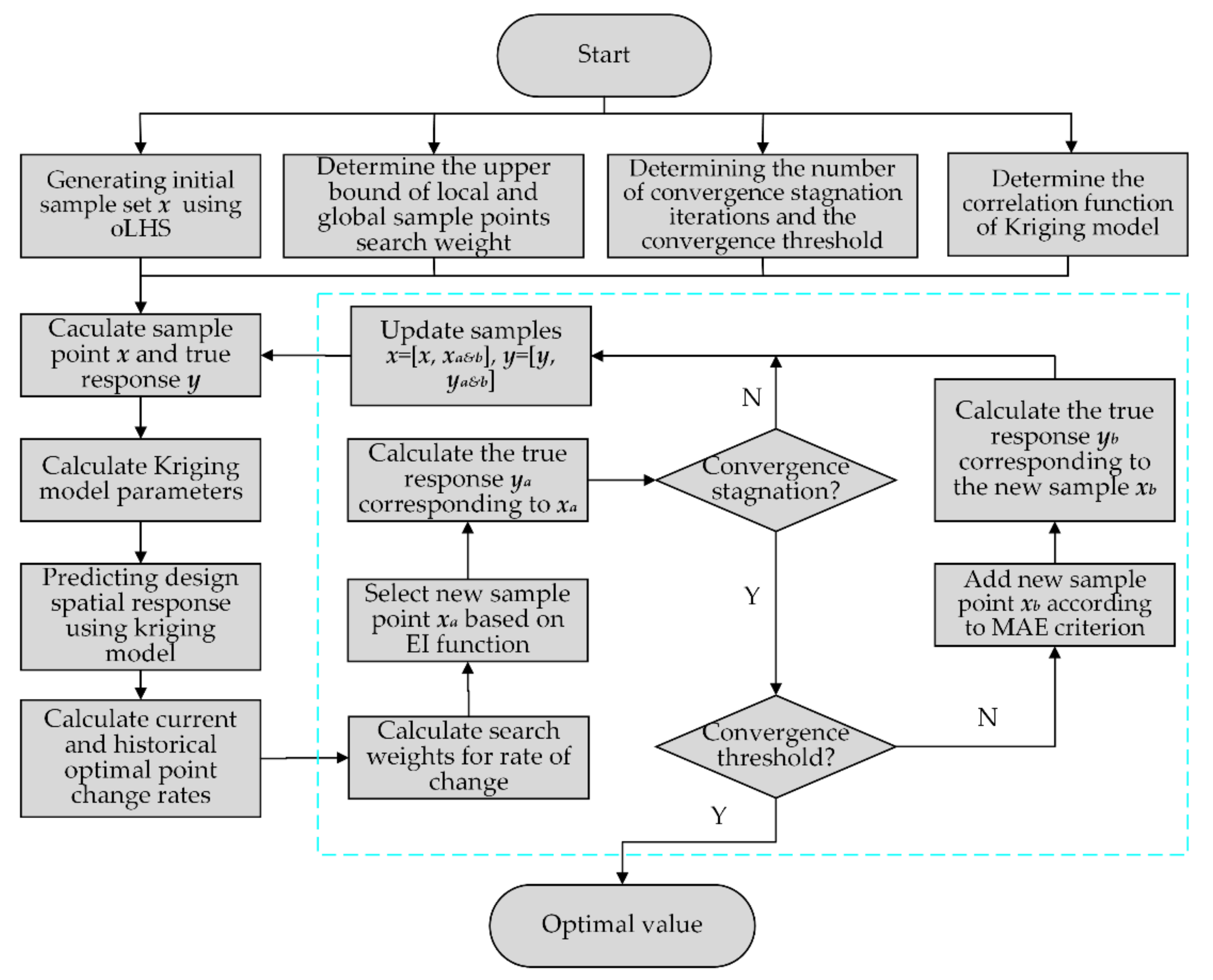
Equation (11) shows that the weight assigned by the traditional EGO algorithm to the first and second terms of the EI function is one, which means that during the whole optimization search process, when the current optimal point continues to converge, the EGO algorithm cannot determine whether the current optimal point is a global optimal point, so it may fall into the trap of local convergence or lead to very slow convergence later. Therefore, this paper presents an improved EGO (IEGO) algorithm: (1) at the beginning of the search to enhance the search of global sample points and expand the search scope; (2) in the search process, Kriging’s current optimal change range is associated with the search weights of local and global sample points, that is, when the change range is large, the global search weight will also increase, expanding the global search ability. When the optimal change range is small, it means that the IEGO algorithm may find the global optimum and need to refine the local search, so the global search weight will also decrease synchronously; (3) When the convergence stops, increase the sample points (marked as Minimize Absolute Error, MAE criterion) with a large error between the predicted and true values of the surrogate model to improve the accuracy of the Kriging surrogate model. The pseudo-code for IEGO is as follows, and the flow is shown in
Figure 14.
Step 1: Determining the upper search weight limits for local and global sample points, determining the stagnation convergence algebra and convergence threshold, and the correlation function of the Kriging surrogate model;
Step 2: Determine the initial sample points x (using Optimal Latin Hypercube Sampling) and the corresponding outputs y;
Step 3: Using the initial sample to generate the Kriging surrogate model, the parameters of the Kriging model, i.e., the weighting factor , are calculated. The DACE (Design and Analysis of Computer Experiments) toolbox is used to generate the Kriging surrogate model in this paper;
Step 4: Based on the EI criterion and the numerical optimization algorithm (e.g., DE), the Kriging surrogate model is used to determine the EI function in the design space;
Step 5: Calculate the current and historical average optimal change rates, and determine the corresponding search weight. The corresponding relationship between the two can be set as linear; that is, when the change rate is greater than the set stagnation threshold, the search weight is reset to the maximum. When the change rate decreases, the search weight decreases synchronously. When the change rate is close to 0, the search weight is reset to the minimum value of 0; that is, the RMSE infill criterion is adopted, the optimum model of the RMSE infill criterion is:
Step 6: Determine the new sample point xa and calculate the corresponding true output ya;
Step 7: Determine if the result iteration is stalled. If convergence occurs, skip step (8), otherwise skip Step 10;
Step 8: Determine if the convergence threshold is met. If satisfied, skip step (11), otherwise skip Step 9;
Step 9: Add a new sample point xb according to the MAE criterion and calculate the corresponding real output yb;
Step 10: Update the sample set x = [x, xa&b], y = [y, ya&b], and then skip Step 3;
Step 11: Output the optimal solution and the true value.
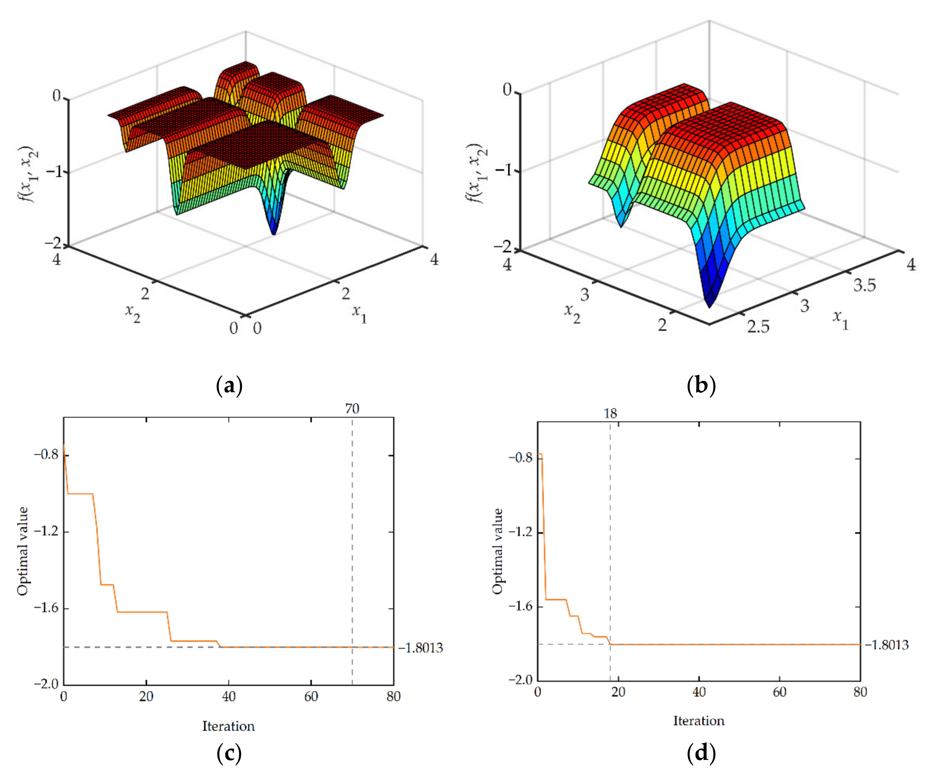
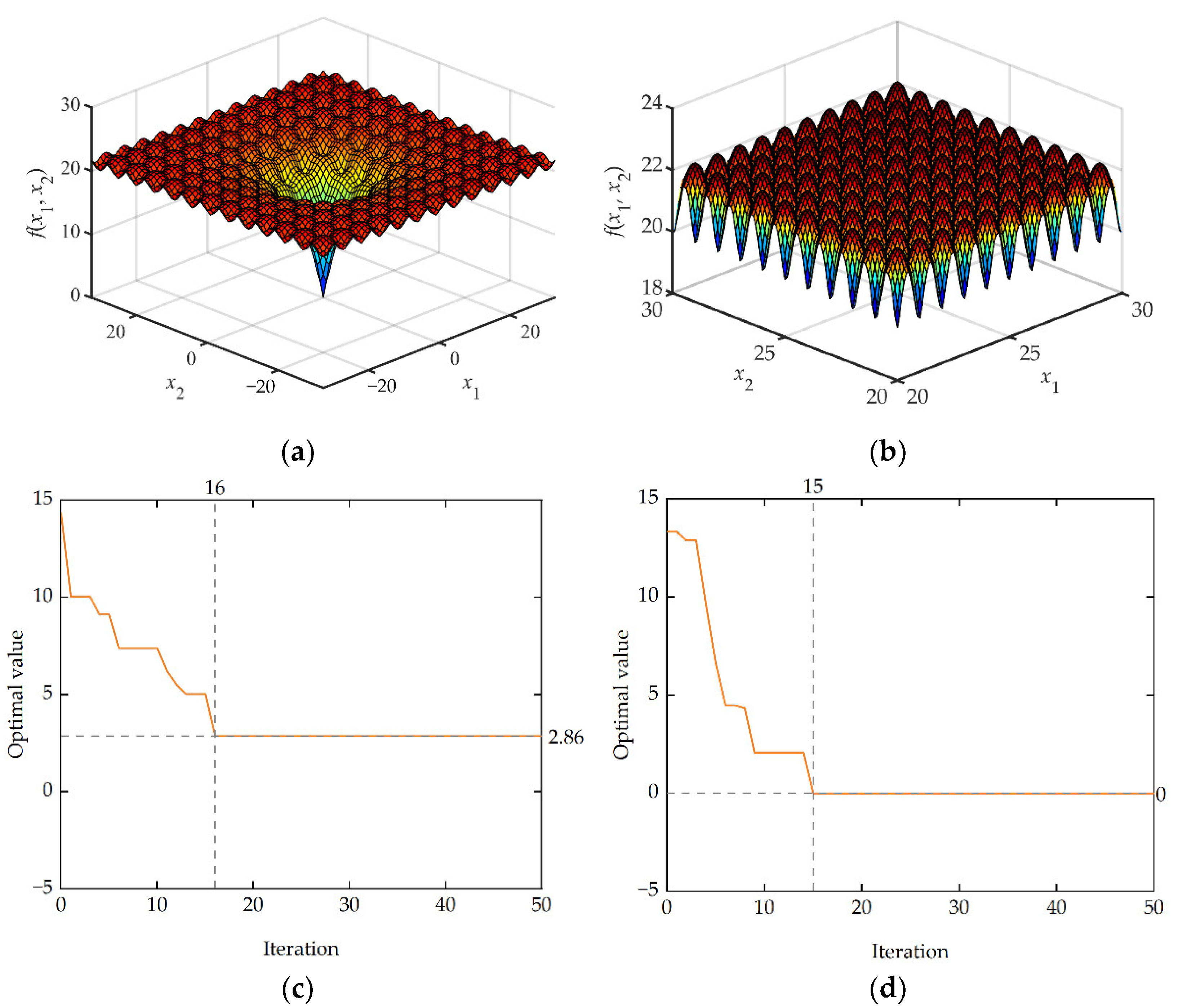
This paper uses two benchmark functions, Michalewicz (
Figure 15a,b) and Ackley (
Figure 16a,b), to test and verify the efficiency and accuracy of IEGO. The specific expressions for benchmark functions, test characteristics, and algorithm settings for this article are given in
Appendix B.
For the Michalewicz function, both the traditional EGO algorithm and the IEGO algorithm have found the global optimal. However, since the Michalewicz function is multimodal and has several local minima, the iteration curve of the algorithm shows that the traditional EGO algorithm has been trapped in the local minima several times and hovered in it, resulting in a very slow convergence rate until the 70th iteration reaches the global optimal (
Figure 15c). In contrast, because the IEGO algorithm proposed in this paper has strong resistance to the local optimum, its convergence rate is significantly faster than that of traditional EGO and finally converges to a global optimum (
Figure 15d).
As mentioned in
Appendix B, the Ackley function has special properties (a deep hole in the center of a nearly flat outer region, with a large number of local minima distributed at the same time). The Ackley function value under the traditional EGO algorithm can approach the global optimum at the early stage of the optimization phase (
Figure 16c), which is almost impossible for the hill-climbing algorithm to complete, but it will converge locally after several iterations and cannot jump out of local minima. After falling into local convergence, the Ackley function value under the IEGO algorithm can further improve the accuracy of the Kriging surrogate model by adjusting the global search weight and using the RMSE infill criterion, jump out of local convergence quickly, and finally, reach the global optimal (
Figure 16d).
From the above numerical examples, it can be seen that the IEGO method proposed in this paper has the advantages of fast optimization speed and strong global optimization ability compared with the traditional EGO algorithm.
4.3. Optimization of Interface Contact Pressure
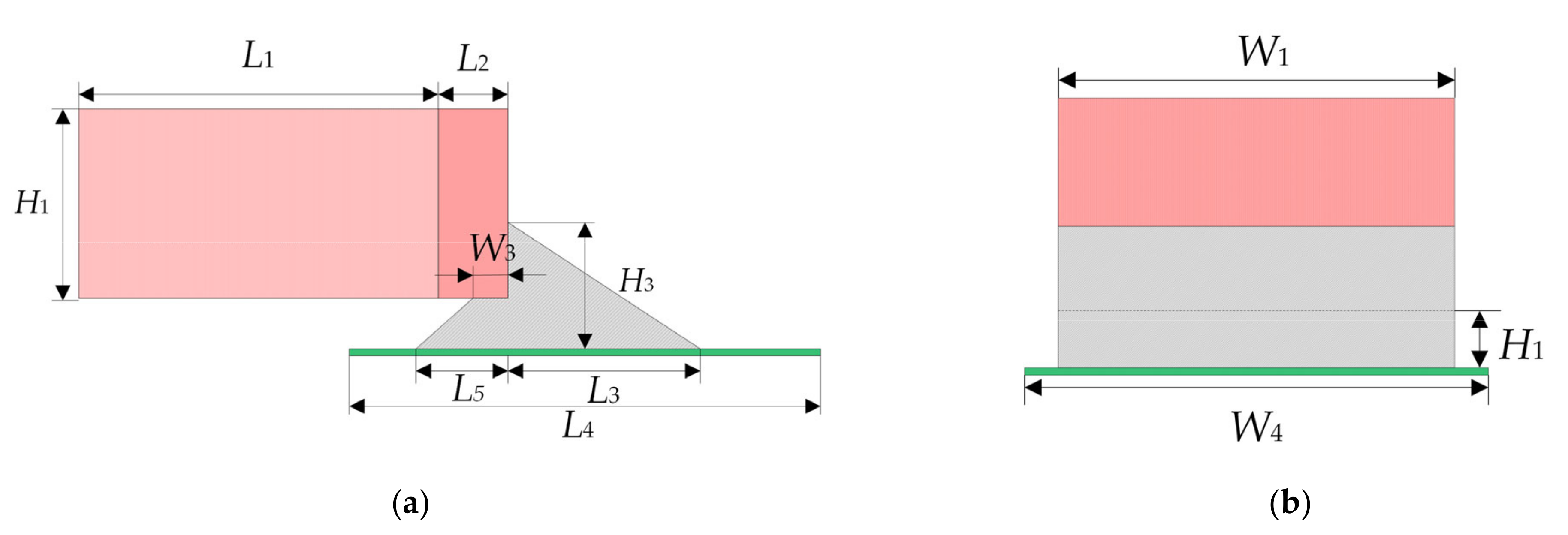
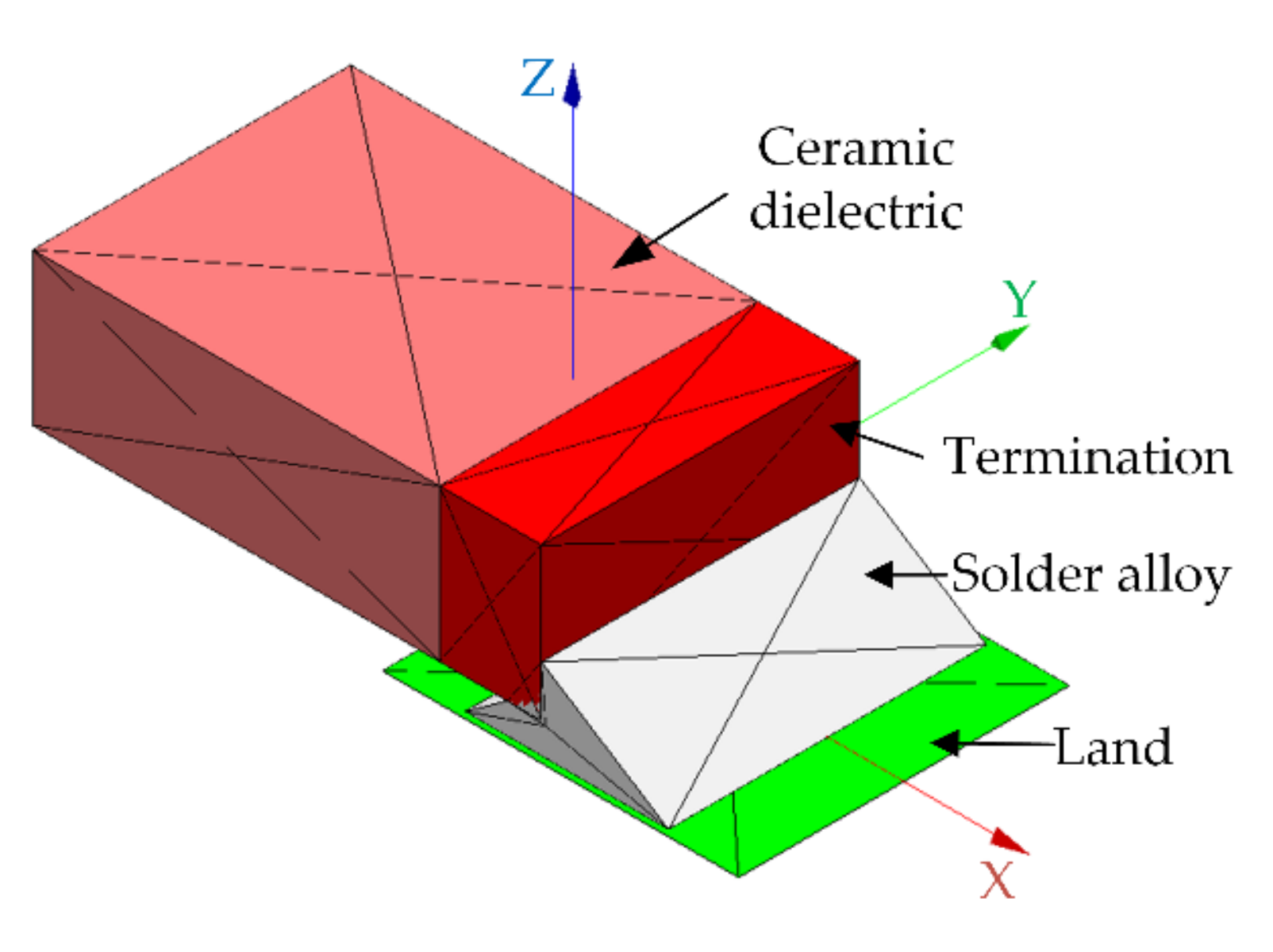
SMT solder joints are easy to be delaminated between pins and lands of components under the thermal load in a service environment. The shape of solder joints has a significant and complex effect on the interface delamination. Therefore, the optimum variables in this paper are the height of solder joints
, the wetting length
and the gap
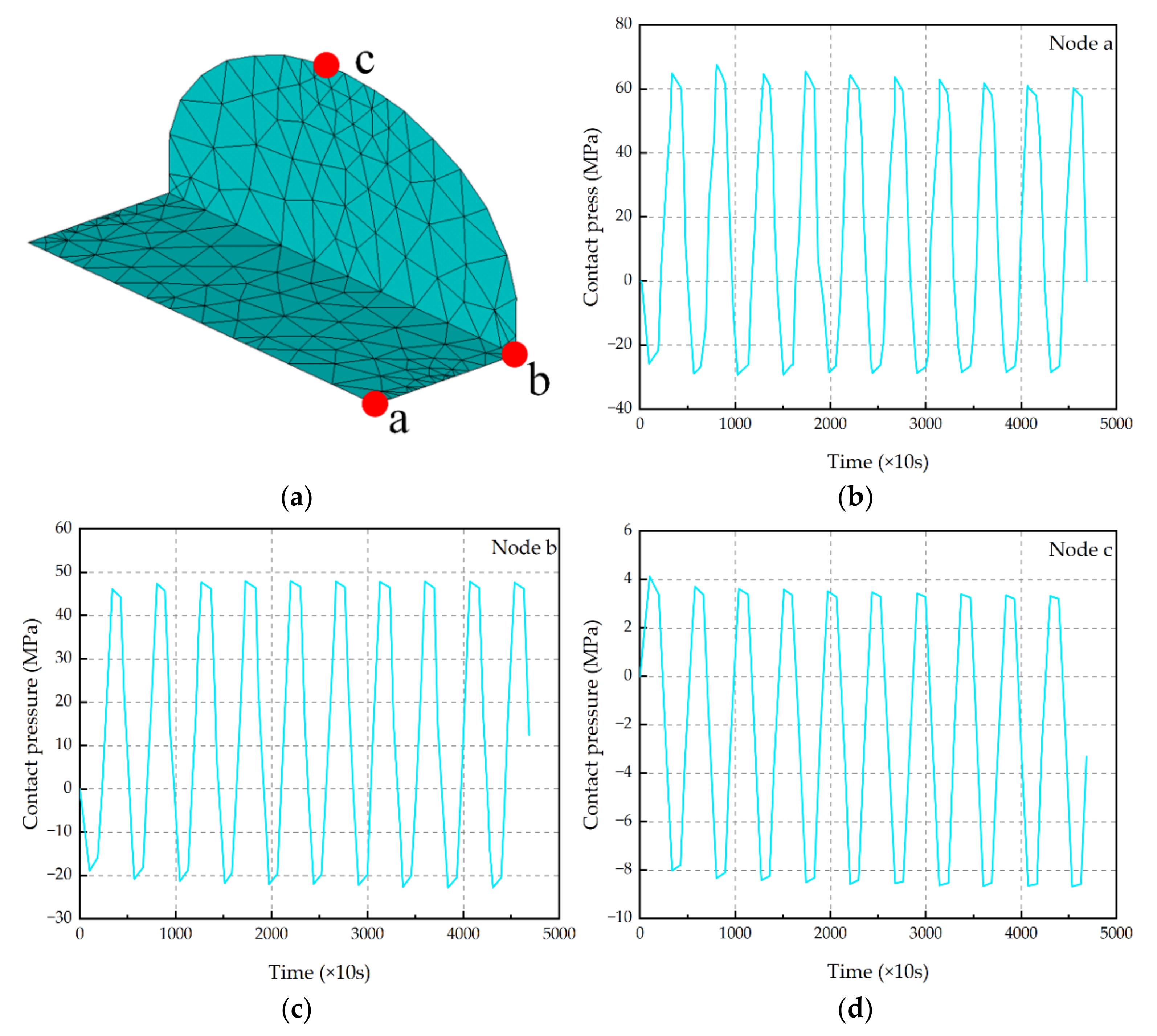
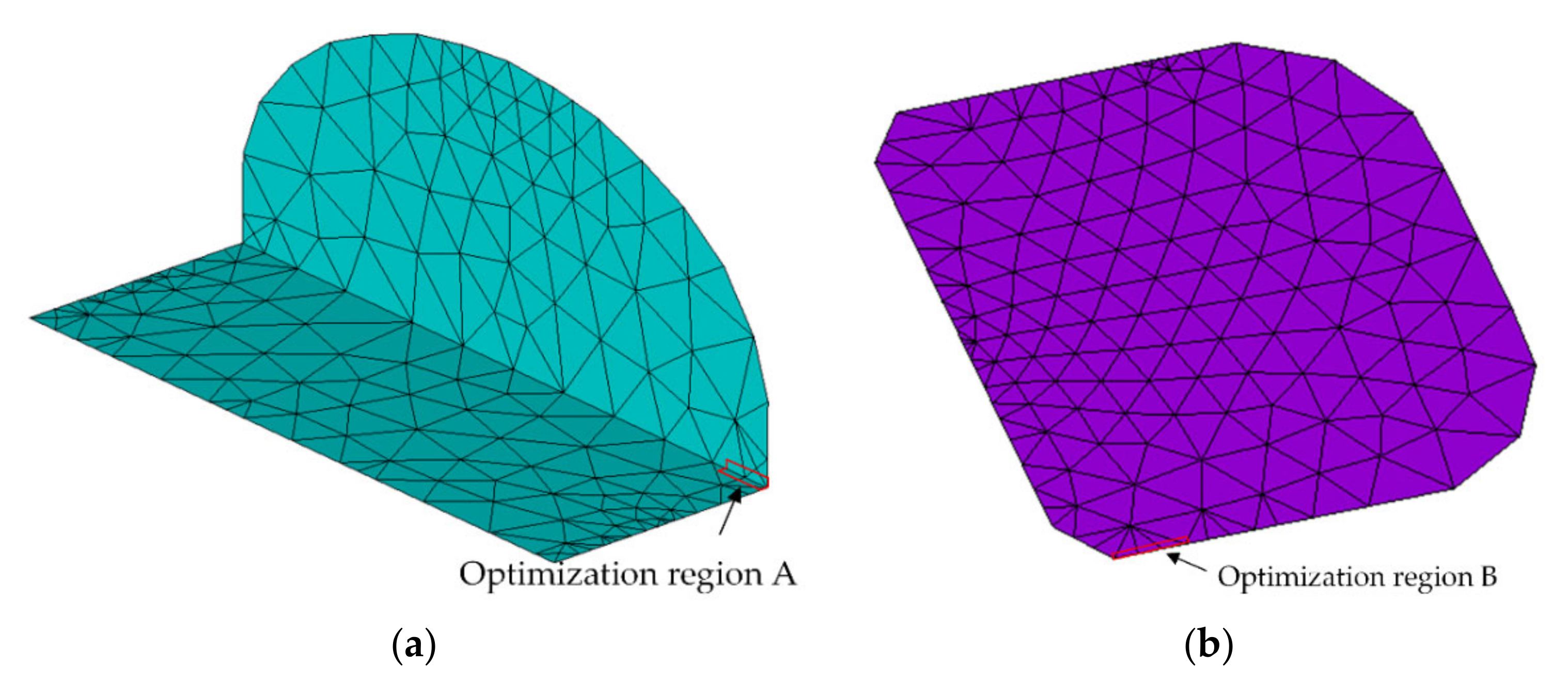
. The interface contact pressure can directly reflect the difficulty of interface delamination, so the interface contact pressure is the optimization target. At the same time, this paper optimizes not only for dangerous points but also for dangerous areas. According to the analysis in
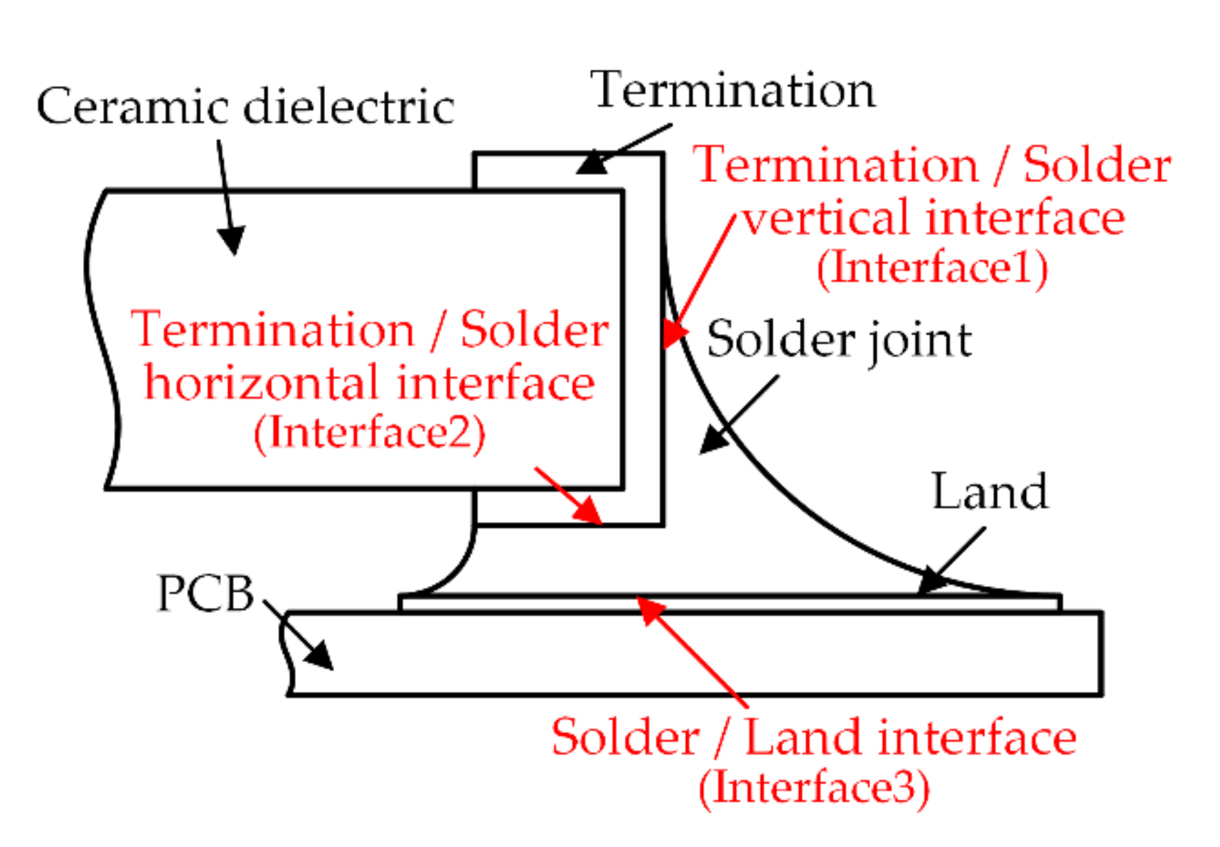
Section 2, for interface 1 and interface 2, it is easier for solder joints to be delaminated at the interface between the two interfaces and the terminations. In this paper, the maximum contact pressure at the solder of interface 1 and interface 2 and the average contact pressure of all nodes with a width of 0.02 mm and a depth of less than 0.06 mm are predicted. The optimization range is shown in
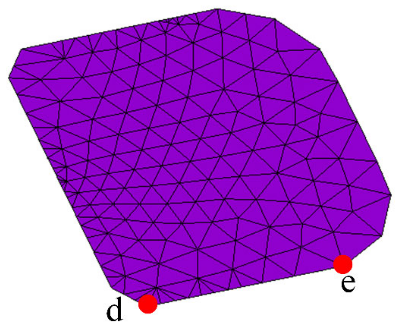
Figure 17a. At the same time, for interface 3, solder joints are most easily stratified on both sides of interface 3 and the land. The maximum contact pressure on both sides of interface 3 and the average contact pressure of all nodes with a width of less than 0.1 mm are also optimized in this paper. The optimization region is shown in
Figure 17b.
Therefore, the target of optimization is not only the contact pressure
and
of nodes b and d, but also the average contact pressure
and
of all nodes in delaminated area A and B. Because the four indexes have different degrees of influence on the SMT solder delamination, the weighting coefficients
,
,
and
are introduced, and the sum of the weighting coefficients is 1, based on the analysis of contact pressure of dangerous nodes in
Section 2, the weighting coefficients of each item are set to
,
,
,
, respectively. Establish optimization model:
where
and
represent the extreme value of the interval of the solder height, respectively.
and
represent the extreme values of the wetting length of the solder joints, respectively.
and
represent the extreme values of the interval between the gap of the solder joints, respectively.
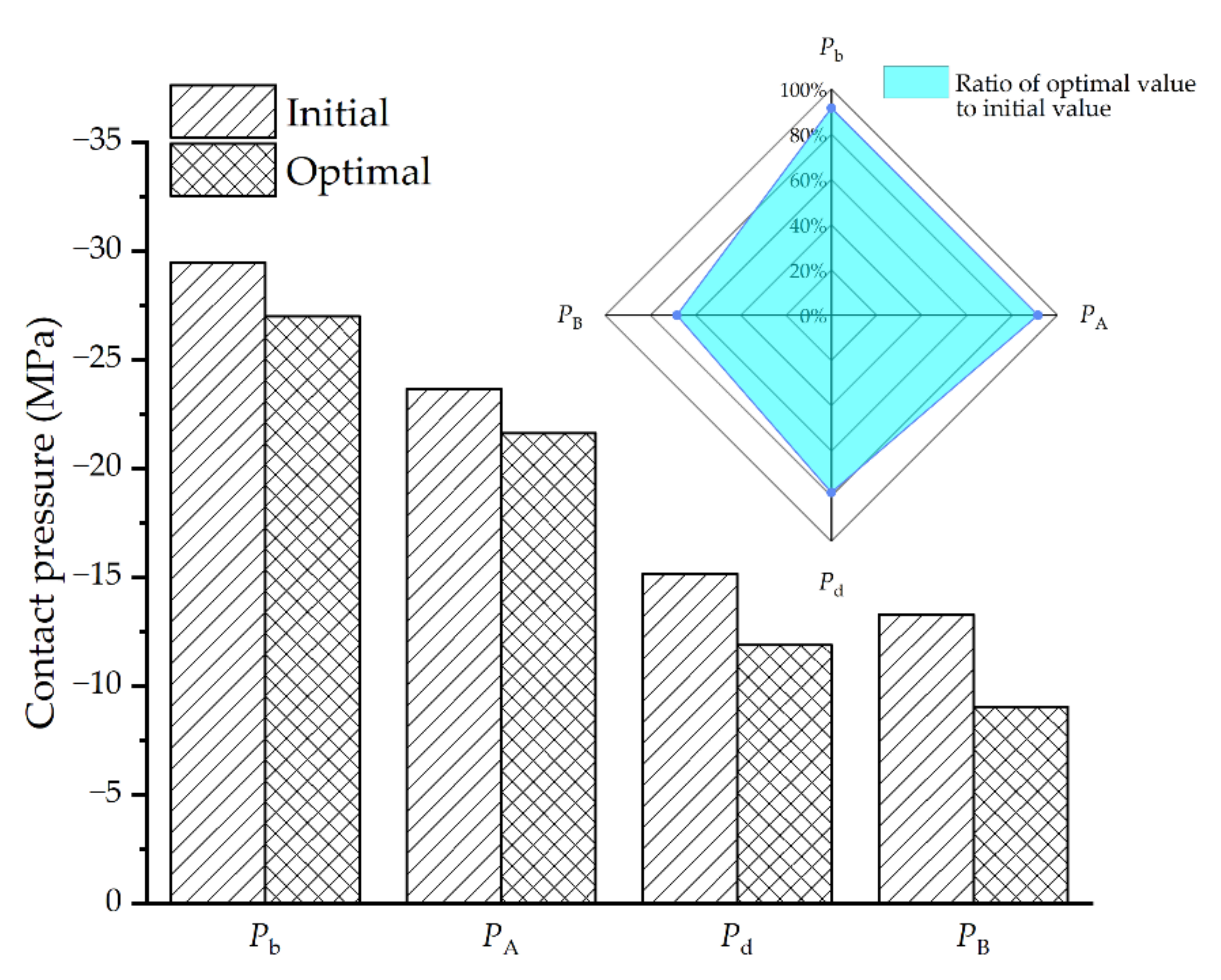
Based on the IEGO algorithm proposed in this paper, the above optimization model is solved, and the contact pressure values of each node and critical region in the optimization model are obtained by the high-cost FEA described above. The optimum geometric parameters of the solder joint are shown in
Table 6. Correspondingly, the contact pressure of each critical point and critical region under this optimal combination of parameters is shown in
Figure 18. Specifically, the contact pressure of
is −27.01 MPa,
is −21.63 MPa,
is −11.89 MPa,
is −9.06 MPa, compared with the initial geometric parameters, the contact pressure of
decreases by 8.38%, that of
by 8.62%, that of
by 21.6%, and that of
by 31.7%.


 ,
, 

