Biomimetic-Based Output Feedback for Attitude Stabilization of Rigid Bodies: Real-Time Experimentation on a Quadrotor

Abstract

The present paper deals with the development of bounded feedback control laws mimicking the strategy adopted by flapping flyers to stabilize the attitude of systems falling within the framework of rigid bodies. Flapping flyers are able to orient their trajectory without any knowledge of their current attitude and without any attitude computation. They rely on the measurements of some sensitive organs: halteres, leg sensilla and magnetic sense, which give information about their angular velocity and the orientation of gravity and magnetic field vectors. Therefore, the proposed feedback laws are computed using direct inertial sensors measurements, that is vector observations with/without angular velocity measurements. Hence, the attitude is not explicitly required. This biomimetic approach is very simple, requires little computational power and is suitable for embedded applications on small control units. The boundedness of the control signal is taken into consideration through the design of the control laws by saturation of the actuators’ input. The asymptotic stability of the closed loop system is proven by Lyapunov analysis. Real-time experiments are carried out on a quadrotor using MEMS inertial sensors in order to emphasize the efficiency of this biomimetic strategy by showing the convergence of the body’s states in hovering mode, as well as the robustness with respect to external disturbances.

1. Introduction

Flapping flyers perform different types of maneuvers during their flight based on information provided by their sensitive organs. This information allows the animal to control its own equilibrium, to orient itself in its environment and to interact with it, as well as to perform tasks. The sensitive organs of an insect, for example, comprise visual sensors, such as the ocelli and the compound eyes, besides other biological sensors, such as halteres, sensilla and magnetic sense [1,2,3].

Specialists claim that flight control commands involved in insect flight originate in the fly’s brain, which has 3000 nerve cells, or neurons [3]. However, these three thousand neurons, each interpreted as an on-off (binary) transistor, give no more computational power than possessed by a toaster [4]. Despite the above-mentioned aspects, insects are more agile than modern aircraft equipped with super-fast digital computers. Consequently, and as is proposed in [4], flight control from the insect flight perspective represents a paradigm change with respect to conventional flight control, used by manned and unmanned aircraft systems. Currently, conventional flight controls use few measurements and many computations, whereas insects flight control does the opposite: many measurements issued from multiple sensors and little computation.

Adopting this strategy, the insect determines its trajectory and adapts its body’s velocity and attitude to track it. Given the maneuverability of flying insects, it is natural to look to biology to get inspiration from their attitude control strategies and to mimic them. Attitude control concerns a wide variety of robotic applications in scenarios aiming to ensure orientation stabilization or trajectory tracking. Moreover, it is a major step that helps to guarantee the position stabilization of underactuated systems where the translational and rotational degrees of freedom must be coupled in order to achieve movement in 3D space. Some illustrative examples for the application include micro-satellites, unmanned aerial vehicles (UAVs), autonomous underwater vehicles (AUVs), etc.

Many approaches have been reported in the literature to develop attitude stabilizing control laws for various applications [5,6,7,8,9,10,11,12,13]. The list is far from being exhaustive. Although the aforecited strategies have solved the attitude stabilization problem, they are based on state feedback: the attitude, represented by the Euler angles in ${\mathbb{R}}^3$, the quaternion in ${\mathbb{S}}^3\subset {\mathbb{R}}^4$ or the rotation matrix in SO(3) [14] and the angular velocity in ${\mathbb{R}}^3$, which are supposed to be known. Since a direct measurement of the attitude is not possible, the information about attitude is obtained through adequate observers (attitude estimators) that combine sensor measurements (see [15,16,17,18] and the references therein). The sensors used for attitude determination can be classified into two main categories: (i) the angular velocity sensors (i.e., rate gyros) that give the measurement of the angular velocity; and (ii) the reference vector sensors (i.e., magnetometers, accelerometers, star trackers, sun sensors) that give the projection, in their local frame, of a fixed vector in space. This projection is known as “vector observation”. Nowadays, there exist many commercial attitude units that are based on these type of sensors and attitude estimators. However, the attitude estimator algorithms require powerful computing capacities, which makes them inconvenient for embedded applications with weight or computer power restrictions. Moreover, these strategies are not inspired by natural flight, which is based directly on sensor measurements.

In recent years, a considerable amount of effort has been dedicated to solving the problem of rigid body attitude stabilization by means of inertial pointing, where, similarly to the present work, the control laws are based on direct measurements of the vector reference sensors (e.g., no attitude representation is needed). This problem has been studied under various assumptions and scenarios; for instance, requiring angular velocity measurements as in [19,20,21,22,23,24], in the absence of angular velocity measurements in an aerospace framework [25] and in an aerial-robotics framework [26]. On the other hand, the aerodynamic forces developed by the flapping flyer’s wings are bounded because of the boundedness of the flapping wings’ angles. Technically, it is well known that for a system that operates over a wide range of conditions, it may happen that the control law reaches the actuator limits, deteriorating the control performance or even leading to instability [27,28]. As evidenced by the above reviewed literature, very little attention has been dedicated to the attitude stabilization problem using bounded control with different bounds for each axis.

Among possible applications, a quadrotor mini-aircraft is used in the present work to test the biologically-inspired control torque computed over sensor measurements that mimic the sensitive organs used by insects. The quadrotor is an under-actuated nonlinear dynamic system having four input forces (delivered by the four propellers (see Figure 3)) and six output coordinates (attitude and position). Mathematically, it gives rise to two cascaded subsystems: rotational and translational ones. The longitudinal and lateral movements cannot be performed without a coupling to the rotational degrees of freedom. Therefore, an efficient attitude control is crucial to maintaining a desired attitude in order to reach a desired position despite the external disturbance. Some linear and nonlinear control techniques have been applied for the attitude stabilization of the quadrotor mini-helicopter, for example [29,30,31,32,33,34,35]. Actually, the control laws previously mentioned assume that the system states are available, i.e., attitude (e.g., Euler angles, quaternion, rotation matrix) and angular velocity, which is not the case of the present work.

The present paper deals with the development of biomimetically-inspired control laws aiming to stabilize the attitude of systems falling within the framework of rigid bodies. The inputs of the control laws are the direct measurements of onboard sensors, equivalent to those that an insect is equipped with, without the need for an explicit attitude reconstruction (angles, quaternions or rotation matrix). Hence, unlike conventional approaches, the computational cost used for the attitude estimation/reconstruction is avoided. First, a bounded, continuous and static control law is developed using the measurements of the angular velocity (e.g., halteres) and the attitude error via direct measurement of the reference vector sensors (e.g., leg sensilla and magnetic sense). A second bounded, continuous and dynamic control law is proposed based only on the measurements of the reference vector sensors: information about the angular velocity comes from at least two non-collinear vector observations, without any reconstruction of it. This control law spares the measurements of the angular velocity (halteres) in case this sensitive organ is no longer working. Although the control laws are a function of the vector observations, the stability analysis is carried out on the configuration space SO(3) of the physical rigid body, in order to avoid any reinterpretation. The asymptotic stability of the rigid body subject to the control laws is proven by means of Lyapunov analysis in both cases. The proposed approach is applied to the real-time attitude stabilization of a quadrotor aircraft in hover mode. The angular velocity is obtained using three rate gyros mounted orthogonally (equivalent to the halteres), and the vector observations are obtained from a triaxial accelerometer and a triaxial magnetometer (equivalent respectively to the leg sensilla and the magnetic sense). The two control law capabilities are tested to ensure the stabilization in a desired constant orientation. They show an expected performance in terms of stabilization time and robustness relative to sensor noise and external disturbances. The rest of the paper is structured as follows. Some mathematical preliminaries and the problem statement are presented in Section 2 and Section 3. The control laws are addressed in Section 4 with the stability proofs. The application to quadrotor UAVs is proposed in Section 5, and experimental results are shown in Section 6. Finally, conclusions are addressed in Section 7.

2. Mathematical Background

Consider two orthogonal right-handed coordinate frames: the body coordinate frame, ${\mathbf{E}}^b=[{\overrightarrow{e}}_1^b,{\overrightarrow{e}}_2^b,{\overrightarrow{e}}_3^b]$, located at the center of mass of the rigid body, and the inertial coordinate frame, ${\mathbf{E}}^f=[{\overrightarrow{e}}_1^f,{\overrightarrow{e}}_2^f,{\overrightarrow{e}}_3^f]$, located at some point in space. The rotation of the body frame ${\mathbf{E}}^b$ with respect to the fixed frame ${\mathbf{E}}^f$ is represented by the attitude matrix $R\in \text{SO}(3)=\{R\in {\mathbb{R}}^{3\times 3}:R^{T}R=I,\det R=1\}$. Denoting by $\omega ={\left[{\omega }_1{\omega }_2{\omega }_3\right]}^T$ the angular velocity vector of the body frame ${\mathbf{E}}^b$ relative to the inertial frame ${\mathbf{E}}^f$, expressed in ${\mathbf{E}}^b$, the rotational kinematic and dynamic equations of the rigid body are given by [14]:

$$\begin{array}{ccc}\hfill \dot{R}& =& -{\left[\omega \right]}^{\times }R\hfill \end{array}$$

(1)

$$\begin{array}{ccc}\hfill J\dot{\omega }& =& -{\left[\omega \right]}^{\times }J\omega +\mathrm{\Gamma }\hfill \end{array}$$

(2)

where ${\left[\xi \right]}^{\times }$ is the skew symmetric matrix associated to the axial vector $\xi ={\left[{\xi }_1{\xi }_2{\xi }_3\right]}^T$:

$${\left[\xi \right]}^{\times }=\left[\begin{array}{ccc}0& -{\xi }_3& {\xi }_2\\ {\xi }_3& 0& -{\xi }_1\\ -{\xi }_2& {\xi }_1& 0\end{array}\right]$$

It is worth remembering that ${\left[\xi \right]}^{\times }\chi =\xi \times \chi$, for all $\chi ,\xi \in {\mathbb{R}}^3$. $J\in {\mathbb{R}}^{3\times 3}$ represents the positive-definite constant inertia matrix of the rigid body expressed in the frame ${\mathbf{E}}^b$, and $\mathrm{\Gamma }\in {\mathbb{R}}^3$ is the vector of control torques in ${\mathbf{E}}^b$. These torques depend on the couples generated by the actuators, aerodynamic couples, such as gyroscopic couples, gravity gradient, etc. In this paper, it is assumed that these torques are only generated by the actuators. Equations (1) and (2) describe the rotational motion of a rigid body that has dynamics evolving on the tangent bundle $T\text{SO}(3)$ [36,37].

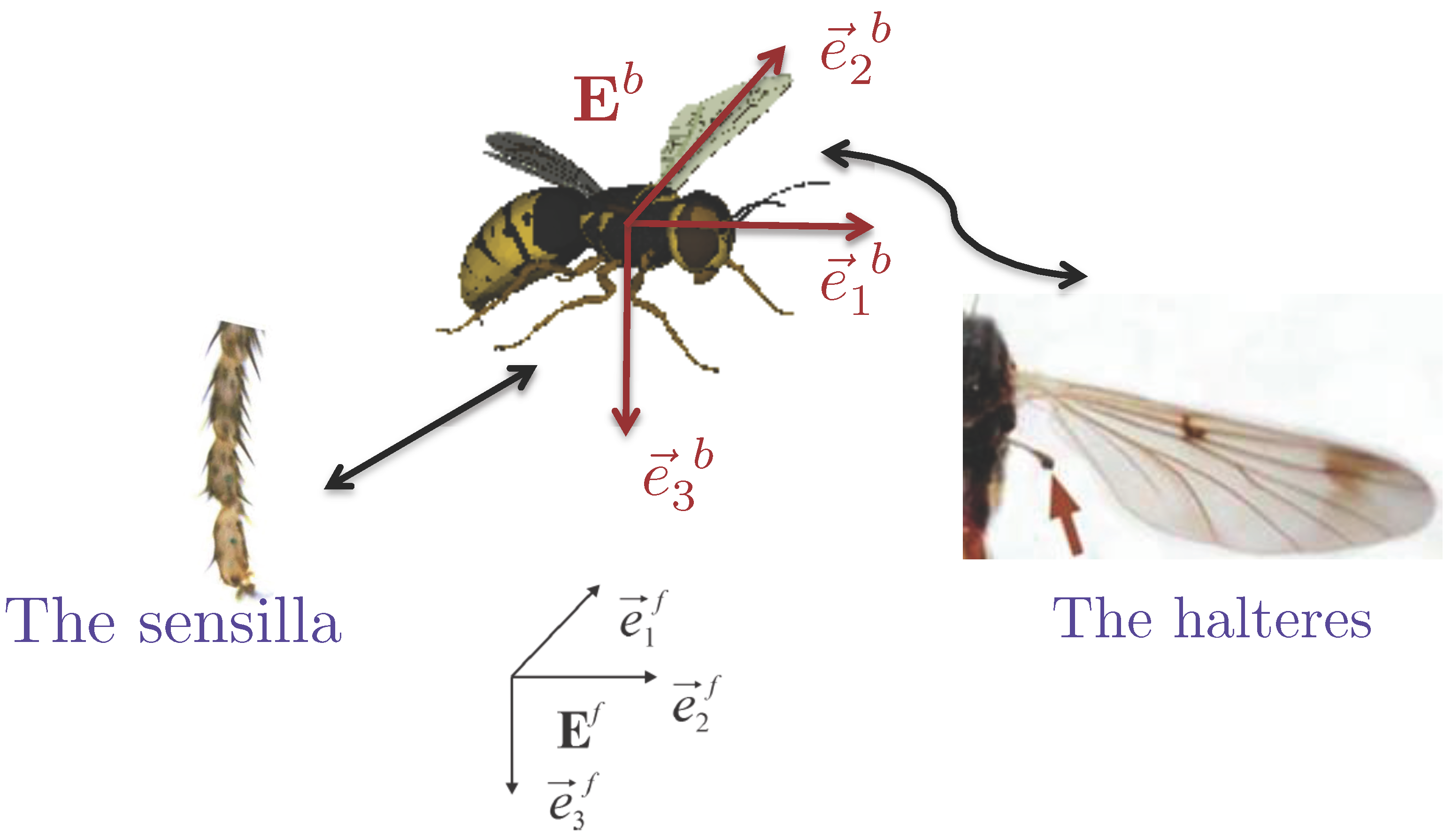
As mentioned in the Introduction, the flapping flyer is provided with information, from multiple sensitive organs. For insects, one can cite the following:

• The halteres: They are gyroscopic biological sensors, located at the wing bases. They allow the detection of the rotational movement of the body and the determination of its angular velocity along the three axes [1,3].
• The sensilla: Located on the antenna, wings and legs, these cuticular sense hairs detect chemical or mechanical stimuli. Particularly, the leg sensilla determine the direction of the gravity field vector with respect to the insect’s body frame [1,3].
• The magnetic sense: This determines the direction of the Earth’s magnetic field vector with respect to the insect’s body frame [1,3].

These three sensitive organs have some technological equivalents: rate gyros, accelerometers and magnetometers, respectively, and they can be divided into two main kinds:

• The angular velocity sensors: These sensors give the measurement of the angular velocity ω. They are assumed to be perfect: problems caused by bias or limited measurement range are not treated in the present work.
• The reference vector sensors: Consider a unit vector ${\overrightarrow{s}}_k$; its representation $s_k^f$ in the fixed frame ${\mathbf{E}}^f$ and $s_k^b$ in the body frame ${\mathbf{E}}^b$. Assume that $s_k^f$ is constant. These two representations are linked up through the rotation matrix R:

  $$s_k^b=R{s}_k^f$$

  (3)

  In attitude control applications, the vectors $s_k^f$ are also called reference vectors and are generally quite accurately known. The body vectors $s_k^b$ are known as “vector observations” and are obtained from on-board sensors (accelerometers, magnetometers, sun sensors, star trackers, etc.). $k\in \{1,2,\dots ,n\}$ represents the number of on-board reference vector sensors. Sensor imperfections are not taken into account in this work.

Vector observations and angular velocity are related through the kinematic Equation:

$${\dot{s}}_k^b={[s_k^b]}^{\times }\omega =-{[\omega ]}^{\times }{s}_k^b$$

(4)

Extending to n vector observations and defining $S^b={(s_1^b{s}_2^b\dots s_n^b)}^T$, it gives:

$$\begin{array}{cc}\hfill {\dot{S}}^b:=\left[\begin{array}{c}{\dot{s}}_1^b\\ ⋮\\ {\dot{s}}_n^b\end{array}\right]& =\left[\begin{array}{c}{\left[s_1^b\right]}^{\times }\\ ⋮\\ {\left[s_n^b\right]}^{\times }\end{array}\right]\omega =:M\omega \hfill \end{array}$$

(5)

The error between the current attitude, defined by a rotation matrix R of the inertial frame ${\mathbf{E}}^f$ axes, and the desired attitude, defined by a rotation matrix $R_d$ of ${\mathbf{E}}^f$’s axes, is quantified by [14]:

$$R_e=R{R}_d^T$$

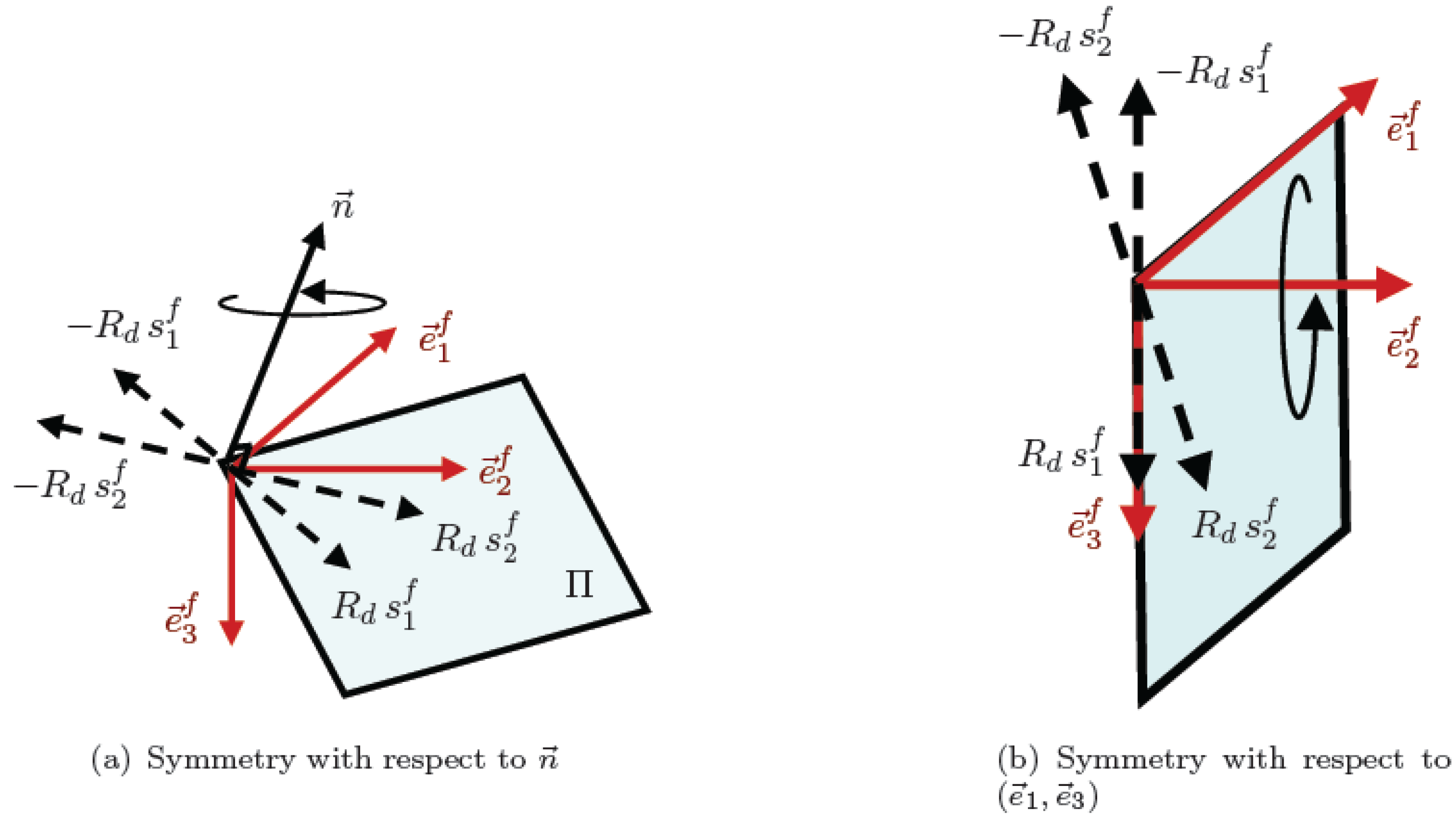
Alternatively, information about the attitude error can be defined as the error between the sensor measurements in the body frame ${\mathbf{E}}^b$ and the desired values of the reference vectors projected in ${\mathbf{E}}^b$. The vector of attitude error γ is defined by:

$$\gamma =\frac{1}{n}\sum _{k=1}^n{[R{s}_k^f]}^{\times }(R_d{s}_k^f)=\frac{1}{n}\sum _{k=1}^n{[s_k^b]}^{\times }{R}_d{s}_k^f$$

(6)

From the perspective of the attitude estimation/determination framework, it is well known that at least two different vector observations at each measurement instant are required in order to obtain complete attitude information [15]. Therefore, to bring the rigid body to a desired orientation, one should nullify the attitude error by forcing γ to zero using at least two non-collinear vectors at each measurement instant, i.e., $n\ge 2$.

Remark 1. 

If only one vector observation is available ($n=1$), this vector is linked to the reference vector, through the rotation matrix R: $s_1^b=R{s}_1^f$. This equation provides a two-dimensional constraint over the three-dimensional rotation matrix. Therefore, a single vector observation does not provide the complete attitude information. In this case, it is impossible to identify a rotation about the axis $s_1^b$ in the body coordinate frame or, equivalently, about the axis $s_1^f$ in the inertial coordinate frame.

Define a scalar saturation function ${\text{sat}}_N(·)$ bounded between $\pm N$, with $N>0$, as:

$${\text{sat}}_N(x)=min(N,max(-N,x)),\forall x\in \mathbb{R}$$

(7)

Define also a vector saturation function for $N=[N_1{N}_2\cdots N_n]$ as:

$${\text{sat}}_N(X)={[{\text{sat}}_{N_1}(x_1)\dots {\text{sat}}_{N_j}(x_j)\dots {\text{sat}}_{N_n}(x_n)]}^T,\forall X=[x_1,\dots ,x_n]\in {\mathbb{R}}^n$$

(8)

with $j\in \{1,\dots ,n\}$ and n is the vector dimension.

3. Problem Statement

The main purpose of the present paper is to design control strategies that would be able to ensure the stabilization of a rigid body’s attitude by mimicking the strategy adopted by flapping flyers to stabilize their attitude. These strategies are based on the use of direct measurements of some sensitive organs, that is the attitude is not explicitly required. Furthermore, the proposed feedback controls take into account the physical constraints and limitations of the body’s structure and actuation. This is ensured by a saturation of the control torque and actually allows the system to avoid unwanted damage and to maximize its effectiveness. This can be mathematically formulated as:

$${\mathrm{\Gamma }}_j\in [-{\overline{\mathrm{\Gamma }}}_j,{\overline{\mathrm{\Gamma }}}_j],j\in \{1,2,3\}$$

where ${\overline{\mathrm{\Gamma }}}_j$ represents the bound of the control torque component ${\mathrm{\Gamma }}_j$ and corresponds to the actuators’ saturation bounds equivalent to the bounds of the aerodynamic torques developed by the flapping flyer’s wings because of the boundedness of the flapping wing angles.

The classical attitude stabilization problem is defined as driving the body’s orientation from any initial condition to a desired constant orientation and maintaining it thereafter. As a consequence, the angular velocity vector is also brought to zero and remains null once the desired attitude is reached.

$$\left\{\begin{array}{cc}R\hfill & \to R_d\\ \omega \hfill & \to 0\end{array}\right.\text{as}t\to \infty$$

The desired and the actual attitudes, $R_d$ and R, are identical if for all $k\in \{1,\cdots ,n\}$ with $n\ge 2$, $s_k^b=R{s}_k^f=R_d{s}_k^f$, and therefore, from Equation (6), $\gamma =0$. However, the reverse is not true, and γ is also minimized for:

$$s_k^b=-R_d{s}_k^f$$

(9)

Analyzing Equality (9) with respect to the number of non-collinear reference vectors n:

• If $n\ge 3$, this identity defines a symmetry with respect to the frame’s origin and can be expressed as $s_k^b=-R_d{s}_k^f$. $-R_d$, however, does not belong to SO(3) and, as a consequence, is not a rotation matrix. Consequently, Equality (9) defines a physically non-feasible configuration. Hence, a null attitude error $\gamma =0$ makes sense only if $s_k^b=R_d{s}_k^f$.
• If $n=2$, there exists a plane Π that contains the vectors $R_d{s}_1^f$ and $R_d{s}_2^f$. The configurations $s_k^b=-R_d{s}_k^f$, $k\in \{1,2\}$, can be reached by a rotation of $180{}^{\circ }(\pi rad)$ about the normal vector $\overrightarrow{n}$ to the plane Π at the vectors’ intersection (Figure 1). Some specific cases of $s_k^f$ allow the definition of symmetry with respect to the separate axes ${\overrightarrow{e}}_1^f,{\overrightarrow{e}}_2^f$, and ${\overrightarrow{e}}_3^f$ if $s_k^f,k\in \{1,2\}$, belong respectively to the planes (${\overrightarrow{e}}_2^f,{\overrightarrow{e}}_3^f$), (${\overrightarrow{e}}_1^f,{\overrightarrow{e}}_3^f$), (${\overrightarrow{e}}_1^f,{\overrightarrow{e}}_2^f$) (Figure 1). In this case, $s_k^b=-R_d{s}_k^f$ is equivalent to $s_k^b=R_s{R}_d{s}_k^f$ with $R_s$ a symmetric matrix that belongs to SO(3) and has a trace $Tr(R_s)=-1$:

  $$R_s\in \{\mathbf{diag}(1,-1,-1),\mathbf{diag}(-1,1,-1),\mathbf{diag}(-1,-1,1)\}$$

  (10)

  defining a symmetry with respect to ${\overrightarrow{e}}_1^f,{\overrightarrow{e}}_2^f$ and ${\overrightarrow{e}}_3^f$, respectively. One should emphasize that it would be therefore more judicious to choose the reference sensors so that the reference vectors belong to one of the three planes (${\overrightarrow{e}}_1^f,{\overrightarrow{e}}_2^f$), (${\overrightarrow{e}}_1^f,{\overrightarrow{e}}_3^f$) or (${\overrightarrow{e}}_2^f,{\overrightarrow{e}}_3^f$), which has been adopted in the present work. If such reference sensors do not exist, another approach would be the definition of the fixed frame with respect to the reference sensors, such that an orthogonalization of the reference vectors is used to construct an ortho-normal basis (${\overrightarrow{e}}_1^f,{\overrightarrow{e}}_2^f,{\overrightarrow{e}}_3^f$).

  Figure 1. Symmetry with respect to the normal vector $\overrightarrow{n}$ to the plane Π (a); the symmetry with respect to the plane (${\overrightarrow{e}}_1^f,{\overrightarrow{e}}_3^f$) (b).

  Figure 1. Symmetry with respect to the normal vector $\overrightarrow{n}$ to the plane Π (a); the symmetry with respect to the plane (${\overrightarrow{e}}_1^f,{\overrightarrow{e}}_3^f$) (b).
• If $n=1$, the symmetry is defined with respect to a plane. This case is not considered in the present work.

As a conclusion, there exist two sets by which the angular velocity ω and the attitude error γ are equal to zero, namely $(\omega ,R)=(0,R_d)$ and $(\omega ,R)=(0,R_s{R}_d)$. Define $\mathcal{E}$ as the union of these two sets:

$$\mathcal{E}=\{(\omega ,R)\in T\text{SO}(3):\omega =0,R=P{R}_d,P\in \mathcal{P}\}$$

(11)

with:

$$\mathcal{P}:=\{\mathbf{diag}(1,1,1),\mathbf{diag}(1,-1,-1),\mathbf{diag}(-1,1,-1),\mathbf{diag}(-1,-1,1)\}$$

(12)

Note that $\mathcal{P}$ forms a subgroup of the group of orthogonal matrices $O(3)$.

4. Biologically-Inspired Attitude Stabilization

In this section, two bounded control laws aiming to stabilize the orientation of a rigid body given by Equations (1) and (2) are proposed. Both control laws (i) are based on an output feedback using on-board sensor measurements and (ii) respect the actuators’ limitation by bounding the developed torque (see Section 2 and Section 3). Vector observations, defining the attitude error, besides the measurement of the angular velocity, are the basis for the first control law computation. This corresponds to the case of accessibility of the halteres, leg sensilla and magnetic sense measurements for an insect (see Figure 2). In the second one, the three rate gyros mounted orthogonally are spared, i.e., the measurements of the halteres are not accessible, and only vector observations are available. This case corresponds, for example, to applications that are limited in terms of aircraft payload or sensor failure. To establish the conditions that guarantee an asymptotic convergence, the geometric configuration of the vector observations is required to satisfy the following assumption.

Assumption 1. 

There are at least two non-collinear vector observations at each measurement instant i.e., $s_k^b$ with $k\in \{1,2,\dots ,n\}$ and $n\ge 2$. The case of the non-existence of these two vectors is admittedly considered beyond the scope of this paper.

Figure 2. Biologically-inspired attitude stabilization.

Figure 2. Biologically-inspired attitude stabilization.

4.1. Bounded Attitude Control with Vector Observations and Angular Velocity Measurements

Theorem 1. 

Consider the rigid body rotational dynamics described by Equations (1) and (2). The attitude error between current and desired orientations is defined by Equation (6) with $n\ge 2$. It is assumed that the body’s angular velocity $\omega ={\left[{\omega }_1{\omega }_2{\omega }_3\right]}^T$ is measured by three rate gyros mounted orthogonally. Define the bounded control $\mathrm{\Gamma }={\left[{\mathrm{\Gamma }}_1{\mathrm{\Gamma }}_2{\mathrm{\Gamma }}_3\right]}^T$ by:

$${\mathrm{\Gamma }}_j=-sa{t}_{N_j}\left({\lambda }_j{\omega }_j\right)-\rho {\gamma }_j,j\in \{1,2,3\}$$

(13)

where ${\overline{\mathrm{\Gamma }}}_j=N_j+\rho$ is the bound of the control torque component ${\mathrm{\Gamma }}_j$, $sa{t}_{N_j}(·)$ is the classical saturation function defined by Equation (7) and ${\lambda }_j,\rho \in {\mathbb{R}}_{>0}$ are tuning parameters, such that $N_j>\rho$ with $\Lambda =diag({\lambda }_j)$. Then, the control torque defined in Equation (13) asymptotically stabilizes the rigid body at $(\omega ,R)=(0,R_d)$ with a domain of attraction equal to $T\text{SO}(3)\backslash \left\{(0,R_s{R}_d)\right\}$.

Before giving the proof of Theorem 1, an analysis of the closed loop system’s equilibrium, using the control law defined in Equation (13), is given:

$$\begin{array}{ccc}\hfill 0& =& -{\left[\omega \right]}^{\times }R\hfill \\ \hfill 0& =& -{\left[\omega \right]}^{\times }J\omega +\mathrm{\Gamma }\hfill \end{array}$$

which yields $\omega =0$ and $\mathrm{\Gamma }=0$, and therefore, $\gamma =0$. Following the analysis given in Section 3, the closed loop system’s equilibrium is given by the set $\mathcal{E}$ defined in Equation (11).

Proof. 

Consider the candidate Lyapunov function V defined by:

$$V(\omega ,R)=\frac{1}{2}{\omega }^{T}J\omega +\frac{\delta }{n}\sum _{k=1}^n[1-{(R{s}_k^f)}^T{R}_d{s}_k^f]$$

(14)

$V(\omega ,R)$ is a continuous and positive definite function on $T\text{SO}(3)$, since $V(\omega ,R)>0$ for all $(\omega ,R)\in T\text{SO}(3)\backslash (0,R_d)$ and $V(\omega ,R)=0$ if and only if $(\omega ,R)=(0,R_d)$.

Note that $s_k^b=R{s}_k^f$, and $s_k^f$ is constant. The derivative of the Lyapunov Function (14) along a solution of the closed loop system is given by:

$$\begin{array}{cc}\hfill \dot{V}(\omega ,R)& ={\omega }^{T}J\dot{\omega }-\frac{\delta }{n}\sum _{k=1}^n{\dot{s}}_k^{b^T}{R}_d{s}_k^f\hfill \\ & ={\omega }^T(-{[\omega ]}^{\times }J\omega +\mathrm{\Gamma })-\frac{\delta }{n}\sum _{k=1}^n{({[s_k^b]}^{\times }\omega )}^T{R}_d{s}_k^f\hfill \\ & ={\omega }^T\mathrm{\Gamma }+\frac{\delta }{n}\sum _{k=1}^n{\omega }^T({[s_k^b]}^{\times }{R}_d{s}_k^f)\hfill \end{array}$$

Replacing in Equation (6), one has:

$$\dot{V}=\sum _{j=1}^3[{\omega }_j(-{\text{sat}}_{N_j}\left({\lambda }_j{\omega }_j\right)-\rho {\gamma }_j)+\delta {\omega }_j{\gamma }_j]$$

Choosing $\delta =\rho$ and since ${\lambda }_j>0$, $j\in \{1,2,3\}$, it follows that:

$$\dot{V}(\omega ,R)=-{\omega }_1{\text{sat}}_{N_1}({\lambda }_1{\omega }_1)-{\omega }_2{\text{sat}}_{N_2}({\lambda }_2{\omega }_2)-{\omega }_3{\text{sat}}_{N_3}({\lambda }_3{\omega }_3)=-{\omega }^T{\text{Sat}}_N(\Lambda \omega )\le 0$$

(15)

Thus, the derivative of the Lyapunov function along a solution of the closed loop system is negative semidefinite.

It is worth remembering that SO(3) is compact. Hence, for any $(\omega (0),R(0))\in T\text{SO}(3)$, the set:

$$\mathrm{\Omega }=\{(\omega ,R)\in T\text{SO}(3):V(\omega ,R)\le V(\omega (0),R(0))\}$$

is a compact, positively-invariant set of the closed loop.

Let E be the set of all of the points for which $\dot{V}(\omega ,R)\equiv 0$. From La Salle’s invariance principle, it follows that all solutions that start in Ω converge to the largest invariant set in E contained in Ω. From Equation (15), $\dot{V}(\omega ,R)\equiv 0$ implies that $\omega \equiv 0$. Then, substituting this last identity into the closed loop system defined by Equations (1) and (2) with the feedback given in Equation (13), one has:

$$E=\{(\omega ,R)\in T\text{SO}(3):\omega \equiv 0,\gamma \equiv 0\}$$

with γ defined in Equation (6).

Thus, following the analysis of the closed loop system’s equilibria, the largest invariant set in E is given by Equation (11), i.e., $E=\mathcal{E}$. The four points given in Equations (11) and (12) correspond to the equilibria of the closed loop system in $T\text{SO}(3)$. Consequently, all trajectories of the closed loop system converge to one of the equilibrium solutions in $\mathcal{E}$. Furthermore, if at $t_0=0$, the solution of the closed loop system lies in $\mathcal{E}$, it remains there for $t>t_0$.

Now, consider separately each equilibrium point of $\mathcal{E}$ defined by Equations (11) and (12). Evaluating the Lyapunov function defined in Equation (14) at these points, one obtains:

$$V(0,R_d)=0\text{and}V(0,R_s{R}_d)=2\delta$$

Actually, the points $(0,R_d)$ and $(0,R_s{R}_d)$ correspond respectively to a minimum $\left(V(0,R_d)=0\right)$ and a local maximum $\left(V(0,R_s{R}_d)=2\delta \right)$ of the Lyapunov function of Equation (14). The derivative $\dot{V}(\omega ,R)$ is equal to zero at these points.

Next, consider any initial condition $(0,{(R_s{R}_d)}^{*})$ different from $(0,R_s{R}_d)$. Then, evaluating the Lyapunov function at these points trivially gives:

$$(0,{(R_s{R}_d)}^{*})\ne (0,R_s{R}_d)\Rightarrow V(0,{(R_s{R}_d)}^{*})<2\delta$$

Since $\dot{V}<0$ outside $\mathcal{E}$, any initial condition outside $\mathcal{E}$ will lead to a decrease of the Lyapunov function and a convergence to an equilibrium point, where V vanishes (as well as $\dot{V}$), that is $(0,R_d)$. Hence, solutions of the closed loop system whose initial conditions are different from $(0,R_s{R}_d)$ converge asymptotically to $(\omega ,R)=(0,R_d)$.

4.2. Attitude Stabilization with Vector Observations and without Angular Velocity Measurements

In this section, a control law free of velocity measurements is developed. It is based only on the vector observations $s_k^b$ and their derivatives with $k\in \{1,2,\dots ,n\}$ and $n\ge 2$. Practically, this solution corresponds to applications where only a triaxial accelerometer (used as an inclinometer) and a triaxial magnetometer are on-board. Then, one has the following result:

Theorem 2. 

Consider the rigid body rotational dynamics described by Equations (1) and (2). The attitude error between current and desired orientations γ is computed through Equation (6). Define the bounded control torque $\mathrm{\Gamma }={\left[{\mathrm{\Gamma }}_1{\mathrm{\Gamma }}_2{\mathrm{\Gamma }}_3\right]}^T$ as:

$$\begin{array}{cc}\hfill \mathrm{\Gamma }& =-\lambda M^{T}Sa{t}_N(v_m)-\rho \gamma \hfill \\ \hfill \dot{\zeta }& =-a{v}_m\hfill \\ \hfill v_m& =\zeta +b{S}^b\hfill \end{array}$$

(16)

with $a,b\in {\mathbb{R}}_{>0}$ the filter parameters and $\lambda ,\rho \in {\mathbb{R}}_{>0}$ the tuning parameters. $Sat(·)$ is defined in Equation (8). The $3n$ vector N is composed by adding n times a vector of strictly-positive saturation levels $\overline{N}=\left[{\overline{N}}_1{\overline{N}}_2{\overline{N}}_3\right]$, that is $N_i:={\overline{N}}_j$ for $i=3(k-1)+j$, $j\in \{1,2,3\}$, $k\in \{1,\cdots ,n\}$. With the above definitions, the dynamic control law defined in Equation (16) asymptotically stabilizes the rigid body at $(\omega ,R,v_m)=(0,R_d,0)$ with a domain of attraction equal to $T\text{SO}(3)\times {\mathbb{R}}^{3n}\backslash \left\{(0,R_s{R}_d,0)\right\}$. Furthermore, the control torque ${\mathrm{\Gamma }}_j$ remains bounded by ${\overline{\mathrm{\Gamma }}}_j$ along each axis.

Before giving the proof of Theorem 2, the idea behind the construction of the feedback defined in Equation (16) is explained. It is assumed that the angular velocity is not measured (no rate gyros are used). Then, one way is to use Equation (5) to reconstruct the angular velocity by means of $\omega =M^{†}{\dot{S}}^b$, where $M^{†}={(M^{T}M)}^{-1}{M}^T$ is the pseudo-inverse matrix of M, and to use it in Theorem 1. This approach has two main drawbacks. First, it requires relatively heavy computations because of the pseudo-inverse matrix. Furthermore, the numerical stability becomes an issue in the case that the sensors’ number increases. Secondly, it also requires the derivation of the vector observations, known to be very sensitive to noise. This problem can be avoided by taking the difference between the signal and its low-pass filtered version, which approximates the derivative for low frequencies [38]. In the present case, this filter is given by the last two Equations of (16) in its state-space realization. The filter’s output is $v_m$, which is one of the arguments of the control torque defined in Equation (16). In fact $v_m$ and the matrix M provide the required damping to achieve asymptotic stabilization. Furthermore, exact knowledge of the angular velocity is not required. Note that the dynamic control law defined in Equation (16) is similar to the one proposed in [39] for attitude tracking. However, in the aforementioned work, the knowledge of the quaternion is necessary, contrary to the proposed feedback.

The state of the system defined by Equations (1) and (2) subject to the control described in Equation (16), in a closed loop, evolves in $T\text{SO}(3)\times {\mathbb{R}}^{3n}$. The analysis of the equilibrium point of this closed loop system yields $\omega =0$ and $\mathrm{\Gamma }=0$. Then, from Equation (5), one obtains ${\dot{S}}^b=0$. The second and third Equations of (16) can be written as ${\dot{v}}_m=-a{v}_m+b{\dot{S}}^b$; then $v_m=0$, and consequently, $\gamma =0$. Using the same arguments of the previous control law, there exist two sets of equilibrium points for the closed loop system, namely $(\omega ,R,v_m)=(0,R_d,0)$ and $(\omega ,R,v_m)=(0,R_s{R}_d,0)$. Given $R_d$ and $s_k^f$, let $\overline{\mathcal{E}}$ denote the set of equilibrium solutions for the closed loop system:

$$\begin{array}{cc}\hfill \overline{\mathcal{E}}=& \{(\omega ,R,v_m)\in T\text{SO}(3)\times {\mathbb{R}}^{3n}:\omega =0,v_m=0,R=P{R}_d,P\in \mathcal{P}\}\hfill \end{array}$$

(17)

with $\mathcal{P}$ defined in Equation (12).

Note that the low-pass filter given by the last two Equations of (16) is equivalent to ${\dot{v}}_m=-a{v}_m+b{\dot{S}}^b$, but does not necessitate the computation of ${\dot{S}}^b$.

Proof. 

Consider the candidate Lyapunov function L:

$$\begin{array}{cc}\hfill L& =\frac{1}{2}{\omega }^{T}J\omega +\frac{\delta }{n}\sum _{k=1}^n[1-{(R{s}_k^f)}^T{R}_d{s}_k^f]+\alpha b^{-1}\sum _{i=1}^{3n}{\int }_0^{v_{m_i}}{\text{sat}}_{N_i}(\sigma )d\sigma \hfill \end{array}$$

(18)

L is a continuous, proper and positive definite function. $\text{sat}(·)$ is the classical saturation function defined in Equation (7) and is obviously Lipschitz. $L(\omega ,R,v_m)>0$ for all $(\omega ,R,v_m)\in T\text{SO}(3)\times {\mathbb{R}}^{3n}$ and $L(\omega ,R,v_m)=0$ if and only if $(\omega ,R,v_m)=(0,R_d,0)$. Since $s_k^f$ is constant and $R{s}_k^f=s_k^b$, the derivative of L along the solutions of the closed loop system, using γ defined in Equation (6), is given by:

$$\begin{array}{lll}\dot{L}& =& {\omega }^{T}J\dot{\omega }-\frac{\delta }{n}\sum _{k=1}^n{\dot{s}}_k^{b^T}{R}_d{s}_k^f+\alpha b^{-1}{\text{Sat}}_N^T(v_m){\dot{v}}_m\hfill \\ & =& {\omega }^T\mathrm{\Gamma }+{\omega }^T\delta \gamma -\alpha a{b}^{-1}{\text{Sat}}_N^T(v_m)v_m+\alpha {\text{Sat}}_N^T(v_m){\dot{S}}^b\hfill \\ & =& {\omega }^T\mathrm{\Gamma }+{\omega }^T\delta \gamma -\alpha a{b}^{-1}{\text{Sat}}_N^T(v_m)v_m+\alpha {\text{Sat}}_N^T(v_m)M\omega \hfill \\ & =& \underset{{\dot{L}}_1\le 0}{\underbrace{-\alpha a{b}^{-1}{\text{Sat}}_N^T(v_m)v_m}}+\underset{{\dot{L}}_2}{\underbrace{{\omega }^T\mathrm{\Gamma }+{\omega }^T\delta \gamma +\alpha {\omega }^T{M}^T{\text{Sat}}_N(v_m)}}\hfill \end{array}$$

Analyzing ${\dot{L}}_2$, it follows from Γ defined in Equation (16) that:

$${\dot{L}}_2=-\lambda {\omega }^T{M}^T{\text{Sat}}_N(v_m)-{\omega }^T\rho \gamma +{\omega }^T\delta \gamma +\alpha {\omega }^T{M}^T{\text{Sat}}_N(v_m)$$

Choosing $\delta =\rho$ and $\alpha =\lambda$, one obtains:

$${\dot{L}}_2=0$$

Consequently, the derivative of the Lyapunov function defined in Equation (18) is given by:

$$\dot{L}={\dot{L}}_1+{\dot{L}}_2=-\alpha a{b}^{-1}{\text{Sat}}_N^T(v_m)v_m\le 0$$

Thus, the derivative of the Lyapunov function along the solutions of the closed loop system is negative semidefinite.

Recall that SO(3) is compact. Hence, for any $(\omega (0),R(0),v_m(0))\in T\text{SO}(3)\times {\mathbb{R}}^{3n}$, the set:

$$\begin{array}{cc}\hfill \mathrm{\Omega }& =\{(\omega ,R,v_m)\in T\text{SO}(3)\times {\mathbb{R}}^{3n}:L(\omega ,R,v_m)\le L(\omega (0),R(0),v_m(0))\}\hfill \end{array}$$

is a compact, positively-invariant set of the closed loop. From La Salle’s invariance principle, it follows that all solutions that start in Ω converge to the largest invariant set in $\overline{\mathcal{E}}$ contained in Ω. $\dot{L}(\omega ,R,v_m)\equiv 0$ implies that $v_m\equiv 0\Rightarrow {\dot{S}}^b\equiv 0\Rightarrow \omega \equiv 0$. Then, substituting this last identity into the closed loop system defined by Equations (1), (2) and (16), one has:

$$\overline{\mathcal{E}}=\{(\omega ,R,v_m)\in T\text{SO}(3)\times {\mathbb{R}}^{3n}:\omega \equiv 0,v_m\equiv 0,\gamma \equiv 0\}$$

with γ defined in Equation (6). Following the same arguments of the proof of Theorem 1, it results that $\dot{L}<0$ outside $\overline{\mathcal{E}}$ given in Equation (17), and the control law acts to ensure the convergence of the solutions of the closed loop system to the equilibrium point $(\omega ,R,v_m)=(0,R_d,0)$ where $L=\dot{L}=0$.

Finally, it is still necessary to check that the control satisfies the saturation constraints. In the following, for two vectors ${\vartheta }_1$ and ${\vartheta }_2$ of the same dimension, ${\vartheta }_1\le {\vartheta }_2$ will mean that for each component i, ${\vartheta }_{1_i}\le {\vartheta }_{2_i}$. Using Equation (16) and the fact that γ is unitary, it follows that:

$$\begin{array}{ccc}\hfill \mathrm{\Gamma }& =& -\lambda M^T{\text{Sat}}_N(v_m)-\rho \gamma \hfill \\ & \le & \lambda \sum _{k=1}^n\left[\begin{array}{c}\left[\begin{array}{cc}|s_{k_3}^b|& |s_{k_2}^b|\end{array}\right]\left[\begin{array}{c}{\overline{N}}_2\\ {\overline{N}}_3\end{array}\right]\\ \left[\begin{array}{cc}|s_{k_3}^b|& |s_{k_1}^b|\end{array}\right]\left[\begin{array}{c}{\overline{N}}_1\\ {\overline{N}}_3\end{array}\right]\\ \left[\begin{array}{cc}|s_{k_2}^b|& |s_{k_1}^b|\end{array}\right]\left[\begin{array}{c}{\overline{N}}_1\\ {\overline{N}}_2\end{array}\right]\end{array}\right]+\left[\begin{array}{c}\rho \\ \rho \\ \rho \end{array}\right]\le \lambda n\left[\begin{array}{ccc}0& 1& 1\\ 1& 0& 1\\ 1& 1& 0\end{array}\right]\left[\begin{array}{c}{\overline{N}}_1\\ {\overline{N}}_2\\ {\overline{N}}_3\end{array}\right]+\left[\begin{array}{c}\rho \\ \rho \\ \rho \end{array}\right]=\left[\begin{array}{c}{\overline{\mathrm{\Gamma }}}_1\\ {\overline{\mathrm{\Gamma }}}_2\\ {\overline{\mathrm{\Gamma }}}_3\end{array}\right]\hfill \end{array}$$

The vector of saturation levels $\overline{N}$ is given as a function of the torque saturation ${\overline{\mathrm{\Gamma }}}_i$ on each axis by:

$$\left(\begin{array}{c}{\overline{N}}_1\\ {\overline{N}}_2\\ {\overline{N}}_3\end{array}\right)=\frac{1}{2\lambda n}\left(\begin{array}{ccc}-1& 1& 1\\ 1& -1& 1\\ 1& 1& -1\end{array}\right)\left(\begin{array}{c}{\overline{\mathrm{\Gamma }}}_1-\rho \\ {\overline{\mathrm{\Gamma }}}_2-\rho \\ {\overline{\mathrm{\Gamma }}}_3-\rho \end{array}\right)$$

(19)

with the following constraint inequality in order to keep the levels real and strictly positive:

$$\left({\overline{\mathrm{\Gamma }}}_i-\rho \right)<\sum _{j\in \{1,2,3\},j\ne i}\left({\overline{\mathrm{\Gamma }}}_j-\rho \right)$$

(20)

Inequality (20) is always fulfilled taking identical ${\overline{\mathrm{\Gamma }}}_j$ on each axis. Note, however, that it is also fulfilled with two identical bounds and a smaller one (which is the case of quadrotor helicopters addressed in Section 5 and Section 6). Therefore, if the torque physical bounds do not satisfy the inequality, it is always possible to artificially change one control bound to obtain an admissible solution.

5. Application to Quadrotor Helicopter

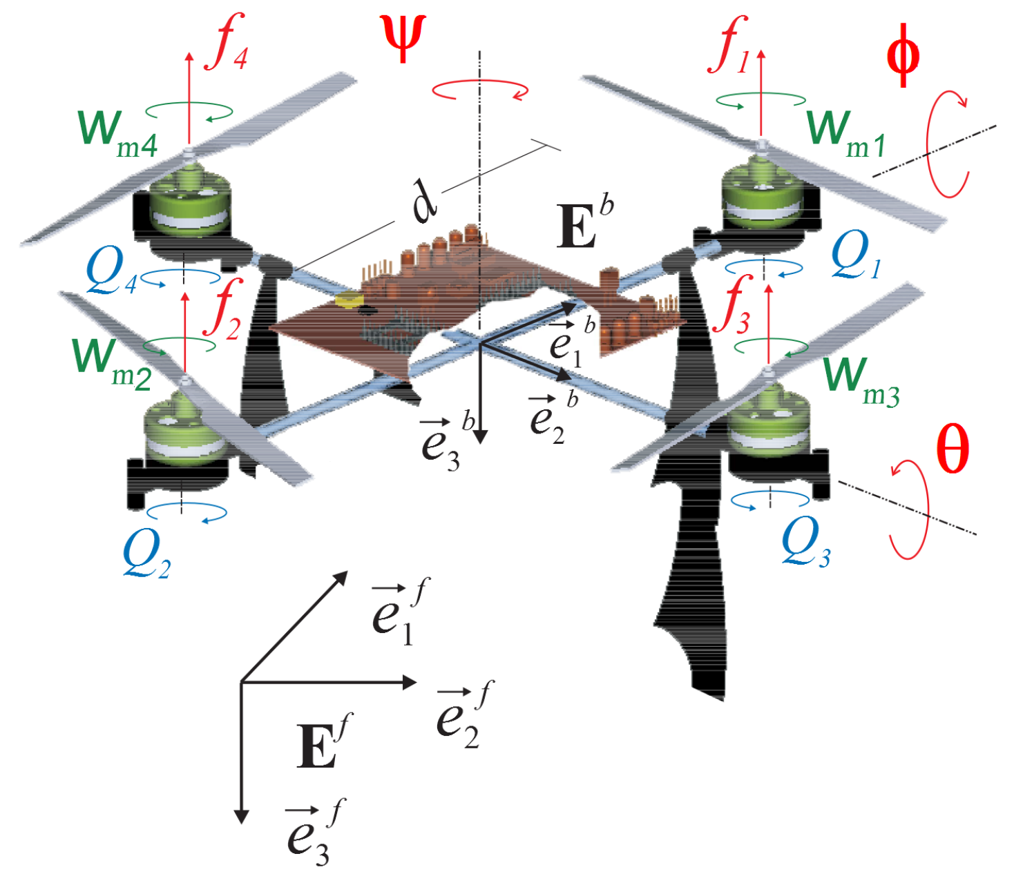
In this section, a quadrotor mini-aircraft is used to test the biologically-inspired control torque proposed in the earlier section. The quadrotor is a small aerial vehicle that belongs to the VTOL (vertical taking-off and landing) class of aircraft, which gives rise to great interest because of its high maneuverability, its payload capacity and its ability to hover. Furthermore, owing to symmetry, it is relatively simple to design and construct. Quadrotors are lifted and propelled, forward and laterally, by controlling the rotational speed of four blades mounted at the four ends of a simple cross and driven by four brushless DC motors (BLDC). On this platform (see Figure 3 and Figure 4), given that the front and rear motors rotate counter-clockwise while the other two rotate clockwise, gyroscopic effects and aerodynamic torques tend to cancel each other out in trimmed flight. The rotation of the four rotors generates a vertical force, called the thrust T, equal to the sum of the thrusts of each rotor ($T=f_1+f_2+f_3+f_4$). The pitch movement θ is obtained by increasing/decreasing the speed of the rear motor while decreasing/increasing the speed of the front motor. The roll movement ϕ is obtained similarly using the lateral motors. The yaw movement ψ is obtained by increasing/decreasing the speed of the front and rear motors while decreasing/increasing the speed of the lateral motors. In order to avoid any linear movement of the quadrotor, these maneuvers should be achieved while maintaining a value of the total thrust T that balances the aircraft weight. In order to model the system’s dynamics, two frames are defined: a fixed frame in the space ${\mathbf{E}}^f=[{\overrightarrow{e}}_1^f,{\overrightarrow{e}}_2^f,{\overrightarrow{e}}_3^f]$ and a body-fixed frame ${\mathbf{E}}^b=[{\overrightarrow{e}}_1^b,{\overrightarrow{e}}_2^b,{\overrightarrow{e}}_3^b]$, attached to the quadrotor at its center of gravity, as shown in Figure 3.

Figure 3. Quadrotor: fixed frame ${\mathbf{E}}^f=[{\overrightarrow{e}}_1^f,{\overrightarrow{e}}_2^f,{\overrightarrow{e}}_3^f]$ and body-fixed frame ${\mathbf{E}}^b=[{\overrightarrow{e}}_1^b,{\overrightarrow{e}}_2^b,{\overrightarrow{e}}_3^b]$.

Figure 3. Quadrotor: fixed frame ${\mathbf{E}}^f=[{\overrightarrow{e}}_1^f,{\overrightarrow{e}}_2^f,{\overrightarrow{e}}_3^f]$ and body-fixed frame ${\mathbf{E}}^b=[{\overrightarrow{e}}_1^b,{\overrightarrow{e}}_2^b,{\overrightarrow{e}}_3^b]$.

According to [40], the six degrees of freedom model (position and orientation) of the system can be separated into translational and rotational motions, represented respectively by ${\Sigma }_T$ and ${\Sigma }_R$ in Equation (21). The quadrotor model can be expressed as:

$${\Sigma }_T:\left\{\begin{array}{c}\begin{array}{cc}\hfill \dot{p}& =v\hfill \\ \hfill \dot{v}& =g{e}_3-\frac{1}{m}{R}^{T}T{e}_3\hfill \end{array}\hfill \end{array}\right.{\Sigma }_R:\left\{\begin{array}{c}\begin{array}{cc}\hfill \dot{R}& =-{\left[\omega \right]}^{\times }R\hfill \\ \hfill J_h\dot{\omega }& =-{\left[\omega \right]}^{\times }{J}_h\omega -{\mathrm{\Gamma }}_G+\mathrm{\Gamma }\hfill \end{array}\hfill \end{array}\right.$$

(21)

where m denotes the mass of the quadrotor and $J_h$ its inertial matrix expressed in ${\mathbf{E}}^b$. g is the gravity acceleration, and $e_3={\left[001\right]}^T$. $p={\left[xyz\right]}^T$ represents the position of the quadrotor’s center of gravity, which coincides with the origin of the frame ${\mathbf{E}}^b$, with respect to the frame ${\mathbf{E}}^f$, $v={\left[v_x{v}_y{v}_z\right]}^T$ its linear velocity in ${\mathbf{E}}^f$, and ω denotes the angular velocity of the quadrotor expressed in ${\mathbf{E}}^b$. ${\mathrm{\Gamma }}_G\in {\mathbb{R}}^3$ contains the gyroscopic torques created by the rotational motion of the quadrotor and the four rotors; $\mathrm{\Gamma }\in {\mathbb{R}}^3$ is the vector of the control torques, and $-T{e}_3$ is the total thrust expressed in ${\mathbf{E}}^b$. Note that the attitude model (rotational motion) of the quadrotor differs from the general rigid body model by means of the gyroscopic torques ${\mathrm{\Gamma }}_G$. R is the rotational transformation from ${\mathbf{E}}^f$ to ${\mathbf{E}}^b$.

The reactive torque $Q_i$ due to the i-th rotor drag, $i\in \{1,2,3,4\}$, and the total thrust T generated by the four rotors can be approximated by an algebraic relationship with the pulse width-modulated (PWM) control signal applied to the BLDC-drivers:

$$Q_i=k_m{u}_{mi}$$

$$T=b_m\sum _{i=1}^4{u}_{mi}=\sum _{i=1}^4{f}_i$$

(22)

where the input signals $u_{mi}$ are expressed in seconds, i.e., the time during which the PWM control signal applied to the motor i is in the high state. $k_m>0$ and $b_m>0$ are two parameters that depend on the air density, the dynamic pressure, the lift coefficient, the radius and the angle of attack of the blades and are experimentally obtained.

Gyroscopic torque ${\mathrm{\Gamma }}_G$ is given by:

$${\mathrm{\Gamma }}_G=\sum _{i=1}^4{J}_r({\left[\omega \right]}^{\times }{e}_3){(-1)}^{i+1}{\omega }_{mi}$$

where ${\omega }_{mi}$ is the rotational speed of rotor i and $J_r$ is the equivalent inertia of the DC motor, the blades and the gear. The components of the control torque vector $\mathrm{\Gamma }={\left[{\mathrm{\Gamma }}_1{\mathrm{\Gamma }}_2{\mathrm{\Gamma }}_3\right]}^T$ generated by the rotors are given by:

$$\begin{array}{l}\begin{array}{ll}{\mathrm{\Gamma }}_1& =d(f_3-f_4)=d{b}_m(u_{m3}-u_{m4})\\ {\mathrm{\Gamma }}_2& =d(f_1-f_2)=d{b}_m(u_{m1}-u_{m2})\hfill \\ {\mathrm{\Gamma }}_3& =-Q_1+Q_2-Q_3+Q_4=k_m(-u_{m1}+u_{m2}-u_{m3}+u_{m4})\hfill \end{array}\end{array}$$

(23)

with d being the distance from one rotor to the center of mass of the quadrotor. Combining Equations (22) and (23), the forces and torques applied to the quadrotor are written as:

$$\begin{array}{c}\hfill \begin{array}{cc}\hfill \left(\begin{array}{c}\mathrm{\Gamma }\\ T\end{array}\right)& =\left(\begin{array}{cccc}0& 0& d{b}_m& -d{b}_m\\ d{b}_m& -d{b}_m& 0& 0\\ -k_m& k_m& -k_m& k_m\\ b_m& b_m& b_m& b_m\end{array}\right)\left(\begin{array}{c}{u}_{m1}\\ u_{m2}\\ u_{m3}\\ u_{m4}\end{array}\right)\hfill \\ & =N{U}_m\hfill \end{array}\end{array}$$

(24)

where $U_m={\left[u_{m1}{u}_{m2}{u}_{m3}{u}_{m4}\right]}^T$. Since N is an invertible matrix, the signals; control is easily obtained.

The specification and parameters of the quadrotor prototype are depicted in Table 1.

Table 1. The specification and parameters of the quadrotor.

Parameter	Description	Value	Units
m	Mass	0.986	kg
d	Distance	0.23	m
$J_{h_{xx}}$	Inertia about ${\overrightarrow{e}}_1^b$	8.13 × 10−3	kg·m2
$J_{h_{yy}}$	Inertia about ${\overrightarrow{e}}_2^b$	8.13 × 10−3	kg·m2
$J_{h_{zz}}$	Inertia about ${\overrightarrow{e}}_3^b$	10.89 × 10−3	kg·m2
$b_m$	Proportionality Constant	5106.8	N/s
$k_m$	Proportionality Constant	342.4	N·m/s

Table 1. The specification and parameters of the quadrotor.

Parameter	Description	Value	Units
m	Mass	0.986	kg
d	Distance	0.23	m
$J_{h_{xx}}$	Inertia about ${\overrightarrow{e}}_1^b$	8.13 × 10−3	kg·m2
$J_{h_{yy}}$	Inertia about ${\overrightarrow{e}}_2^b$	8.13 × 10−3	kg·m2
$J_{h_{zz}}$	Inertia about ${\overrightarrow{e}}_3^b$	10.89 × 10−3	kg·m2
$b_m$	Proportionality Constant	5106.8	N/s
$k_m$	Proportionality Constant	342.4	N·m/s

5.1. Sensors Modeling

The quadrotor is equipped with a sensor suite (MAG-suite) composed of a triaxial magnetometer, a triaxial accelerometer and three rate gyros mounted orthogonally. The MAG-suite represents the sensory system of the insects that is used for their attitude stabilization, i.e., halteres, leg sensilla and magnetic sense.

The MAG-suite’s components are carefully collocated, so that their sensitive axes coincide with the body’s frame ${\mathbf{E}}^b$. The inertial coordinate frame ${\mathbf{E}}^f$ is chosen to be the NED (north, east, down) coordinate frame. In this case, the reference vectors are the gravitational and magnetic vectors. The vector observations, i.e., the gravitational and magnetic vectors expressed in the body frame ${\mathbf{E}}^b$, are obtained from the triaxial accelerometer and the triaxial magnetometer. The angular velocity of the quadrotor is obtained from the three rate gyros. For control purposes, a simple measurement model that does not include a bias term, calibration errors or limited measurement range is considered. As will be shown within the experimental results, the control law is robust with respect to the noise present in these sensor measurements and to external perturbations.

5.1.1. Rate Gyros

The angular velocity $\omega ={\left[{\omega }_1{\omega }_2{\omega }_3\right]}^T$ is measured by three rate gyros mounted orthogonally. That is:

$${\omega }_G=\omega +{\eta }_G$$

where ω is the true angular velocity of the quadrotor and ${\eta }_G$$\in {\mathbb{R}}^3$ is the vector of zero-mean noise supposed bounded.

5.1.2. Accelerometers

The accelerometers measure the difference between the inertial acceleration and gravity expressed in the body frame ${\mathbf{E}}^b$. Then, the triaxial accelerometer’s output can be written as:

$$s_1^b=R(a-g{e}_3)+{\eta }_s$$

where $a\in {\mathbb{R}}^3$ is the projection, in the inertial frame ${\mathbf{E}}^f$, of the acceleration vector $\overrightarrow{a}$ of the body. $g=9.81$ m·s⁻² denotes the gravity acceleration and ${\eta }_s\in {\mathbb{R}}^3$ is the vector of bounded zero-mean noise. If the absolute acceleration of the quadrotor is small relative to the gravity acceleration ($|a|\ll |g{e}_3|$), the “vector observation” given by the accelerometer is:

$$s_1^b=-R{s}_1^f+{\eta }_A$$

(25)

with $s_1^f=g{e}_3/|g{e}_3|={[001]}^T$ and ${\eta }_A={\eta }_s+{\eta }_a$, where ${\eta }_a$ represents the vibrations and small accelerations of the quadrotor.

Remark 2. 

In absence of motion reaction forces exerted by the environment, the quadrotor (or any VTOL vehicle in general) only experiencesacceleration along the body-fixed direction ${\overrightarrow{e}}_3^b$ for the taking-off and horizontal translational movements. In the present case, only the attitude stabilization is studied. Therefore, $|a|\ll |g{e}_3|$ and the triaxial accelerometer can be used as a reference vector sensor where the gravity vector is the reference vector and the acceleration itself is considered as a disturbance. In the case where the translational movements are considered, velocity sensors embedded on the quadrotor can be used to determine the vertical force or thrust and to compute the acceleration subsequently. A compensation of this acceleration in the measurements delivered by the accelerometer can be considered in order to obtain only the projection of the gravity vector in the body’s frame.

5.1.3. Magnetometers

The magnetic field vector expressed in the frame ${\mathbf{E}}^f$ is supposed to be modeled by the unit vector $s_2^f={[0.7100.69]}^T$, which represents the direction of the magnetic field vector in Puebla city, Mexico (GPS: 19°01′41.78′′ N, 98°11′16.81′′ W) where the experiments have been carried out. Since the measurements are relative to the body frame ${\mathbf{E}}^b$, they are given by:

$$s_2^b=R{s}_2^f+{\eta }_M$$

where ${\eta }_M\in {\mathbb{R}}^3$ denotes the perturbing magnetic field supposed to be modeled by zero-mean bounded noise.

Remark 3. 

The quadrotor evolves in a limited space characterized by a constant magnetic field vector.

5.2. Determination of the Unstable Equilibrium

Given the accelerometer sensor measurement $s_1^f={[001]}^T$ and the magnetometer sensor measurement $s_2^f={[0.7100.69]}^T$ (Figure 1), one can easily notice that the two vectors belong to the plane (${\overrightarrow{e}}_1^f,{\overrightarrow{e}}_3^f$). The identity $s_k^b=-R_d{s}_k^f=R_s{R}_d{s}_k^f$ is defined by a symmetry relative to the axis ${\overrightarrow{e}}_2^f$; therefore, $R_s=\text{diag}(-1,1,-1)$, which characterizes a rotation of angle 180° about the axis ${\overrightarrow{e}}_2^f$.

5.3. Bounded Output Feedback for Quadrotor Attitude Stabilization

In order to stabilize the attitude of the quadrotor UAV, the subsystem ${\Sigma }_R$ of Equation (21) is used. The rotational motion of the helicopter responds to the control torques arising from the linear combination of the blades’ rotational speed given in Equation (24). Hence, the maximum airframe control torque depends on the highest rotational speed of the actuators that are used.

Consequently, the maximum torques that can be applied to control the quadrotor’s rotational motion are given by:

$$\begin{array}{ccc}{\overline{\mathrm{\Gamma }}}_1=0.15\mathrm{N}·\mathrm{m},& {\overline{\mathrm{\Gamma }}}_2=0.15\mathrm{N}·\mathrm{m},& {\overline{\mathrm{\Gamma }}}_3=0.09\mathrm{N}·\mathrm{m}\end{array}$$

(26)

In order to avoid unwanted damages to the actuators, the bounded attitude control presented in the previous section is applied to the subsystem ${\Sigma }_R$ of Equation (21).

Corollary 1. 

Consider the quadrotor UAV rotational dynamics described by the subsystem ${\Sigma }_R$ of Equation (21). The bounded control input defined in Equation (13) asymptotically stabilizes the quadrotor at the equilibrium $(\omega ,R)=(0,R_d)$ with a domain of attraction equal to $T\text{SO}(3)\backslash \left\{(0,R_s{R}_d)\right\}$.

Proof. 

The steps of the proof are identical to those of Theorem 1. The only difference lies in the vector ${\mathrm{\Gamma }}_G$, which adds a term that is canceled because of the relation:

$${\omega }^T{\mathrm{\Gamma }}_G={\omega }^T({\left[\omega \right]}^{\times }{e}_3)\sum _{i=1}^4{J}_r{(-1)}^{i+1}{\omega }_{m_i}=0$$

where $J_r$ is the inertia of the rotor.

In the case where the angular velocity is not available, the control law proposed in Theorem 2 can be applied to the quadrotor described by the subsystem ${\Sigma }_R$ of Equation (21). Then, one claims the following result:

Corollary 2. 

Consider the quadrotor mini-helicopter rotational dynamics described by the subsystem ${\Sigma }_R$ of Equation (21). The bounded control input defined in Equation (16) asymptotically stabilizes the quadrotor at the equilibrium $(\omega ,R,v_m)=(0,R_d,0)$ with a domain of attraction equal to $T\text{SO}(3)\times {\mathbb{R}}^{3n}\backslash \left\{(0,R_s{R}_d,0)\right\}$.

Proof. 

The steps of the proof are identical to those of Theorem 2 and Corollary 1.

Remark 4. 

Corollaries 1 and 2 state that the quadrotor can be theoretically asymptotically stabilized from any initial condition belonging to $T\text{SO}(3)\backslash \left\{(0,R_s{R}_d)\right\}$ and $T\text{SO}(3)\times {\mathbb{R}}^{3n}\backslash \left\{(0,R_s{R}_d,0)\right\}$, respectively. However, the stabilization depends on the actuator dynamics. Actually, a quadrotor with sufficient speed and power can fly in a loop without any problem. Nevertheless, hovering or flying in a straight line upside down is quite impossible, since the profile of the blades would not allow this to happen.

6. Experimental Results

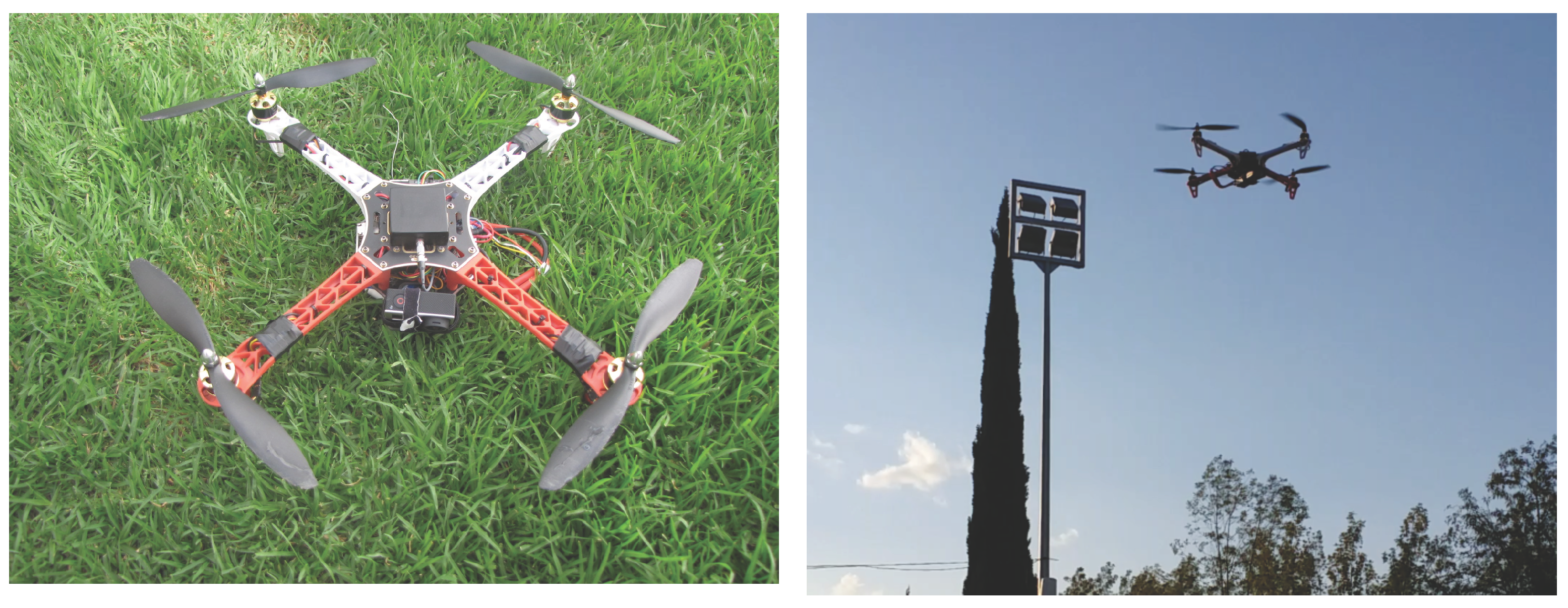
This section is devoted to showing the effectiveness of the proposed control approaches. Experiments on the quadrotor prototype (Figure 4) by the “Dynamical Systems and Control” group of the Autonomous University of Puebla (BUAP) are carried out in real time.

Figure 4. The quadrotor mini-helicopter in flight.

Figure 4. The quadrotor mini-helicopter in flight.

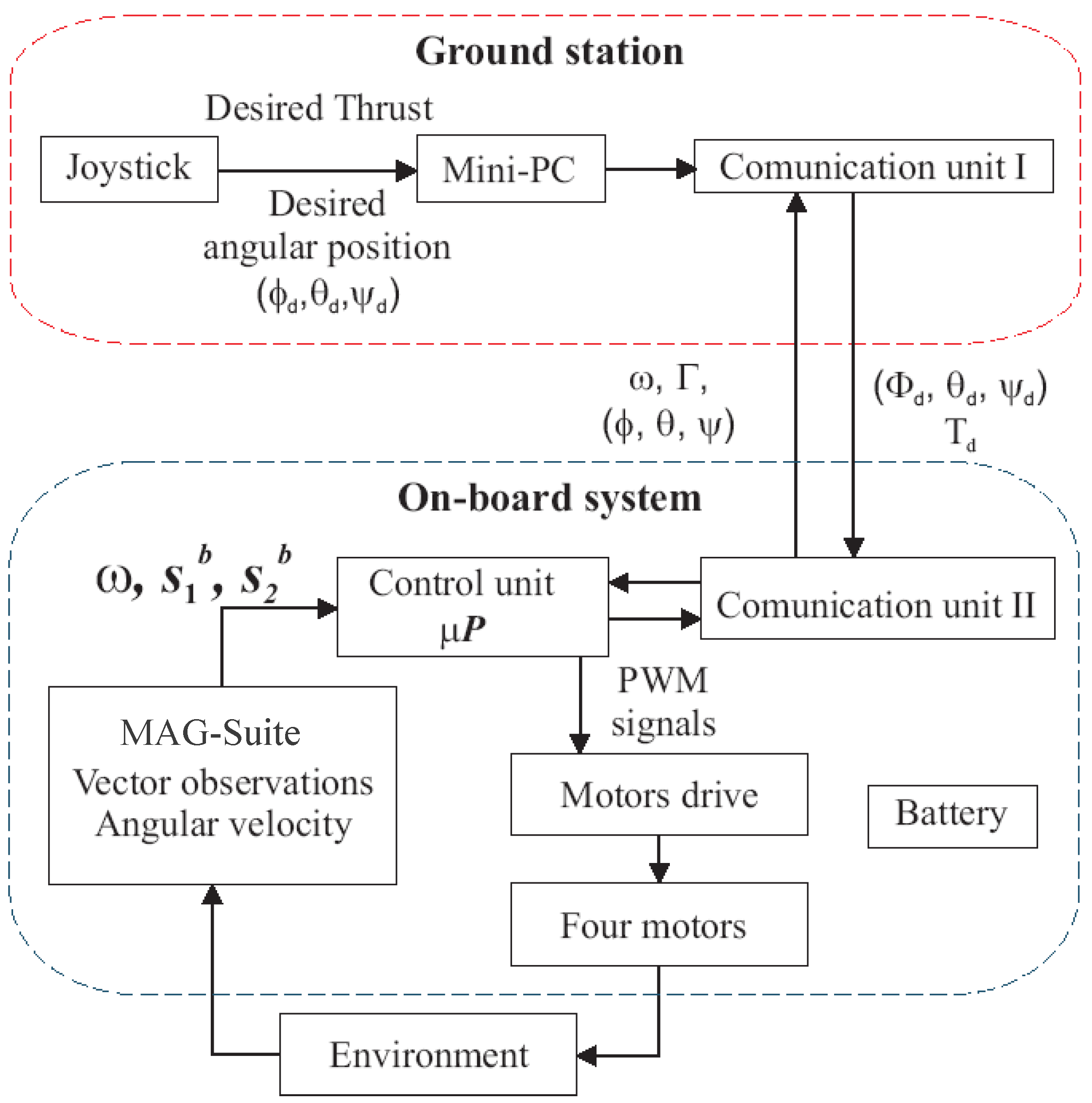
The control laws are executed on a Spartan-6 FPGA LX9 MicroBoard. The Spartan-6 has the ability to implement a “MicroBlaze” soft processor running at 66.7 MHz. Furthermore, the Spartan-6 has the advantage of being able to develop custom modules, such as PWM generators and Universal Synchronous/Asynchronous Receiver/Transmitter (USART) ports. A sensor suite composed of a triaxial magnetometer, a triaxial accelerometer and three rate gyros mounted orthogonally is used to obtain the vector observations and angular velocity by means of a serial communication (RS-232 ). A Bluetooth modem linked to a PC is used to exchange the processed data. The desired attitude can be provided also by means of a five-channel Radio-Control Spektrum DX5e with 2.4-GHz radio technology. Four power modules are used to drive the motors by means of a PWM signal. The frequency of the PWM signal is fixed at 500 Hz. The power for all system is supplied by a 11.1 Volt Li-Po battery, and the total weight is 0.986 kg.

The FPGA inputs are the angular velocity and the vector observations (magnetic and gravity field vectors) provided by the MAG-suite, alongside with the desired attitude provided by the ground station by means of the Bluetooth modem or the Spektrum receiver (in the latter, case a timer detects and measures the width of the pulses coming in from the receiver, which are proportional to the desired angles and desired thrust). Since the desired attitude is provided by the pilot in terms of Euler angles, the on-board processor computes the desired rotational matrix $R_d$ in order to evaluate the attitude error defined in Equation (6). Then, the attitude control law is computed, and the PWM signals used to control the four motors rotational velocities are updated. Optionally, the embedded system can provide the processed data to a ground station, in order to monitor the experiment. The attitude control loop runs at 75 Hz, fixed by the MAG-suite constraints. The block diagram of the overall system is shown in Figure 5.

Figure 5. The block diagram of the quadrotor’s attitude control system.

Figure 5. The block diagram of the quadrotor’s attitude control system.

Two experiments are performed using the control torques defined in Corollaries 1 and 2, respectively, and respecting the motors characteristics given in Equation (26). The objective of the experiments is to bring the quadrotor from any initial orientation to the desired attitude defined by null roll, pitch and yaw angles and to hold it there by maintaining the angular velocity at zero. The desired thrust is taken as $T\ge mg$ = 8.19 N, such that it guarantees a balance of the quadrotor’s weight. Note that the vectors ${\overrightarrow{s}}_1^f$ and ${\overrightarrow{s}}_2^f$ are non-collinear. Furthermore, the direction of ${\overrightarrow{s}}_1^f$ coincides with the direction of the z-axis of the inertial coordinate frame ${\mathbf{E}}^f$.

6.1. Stabilization Using the Control Law of Corollary 1

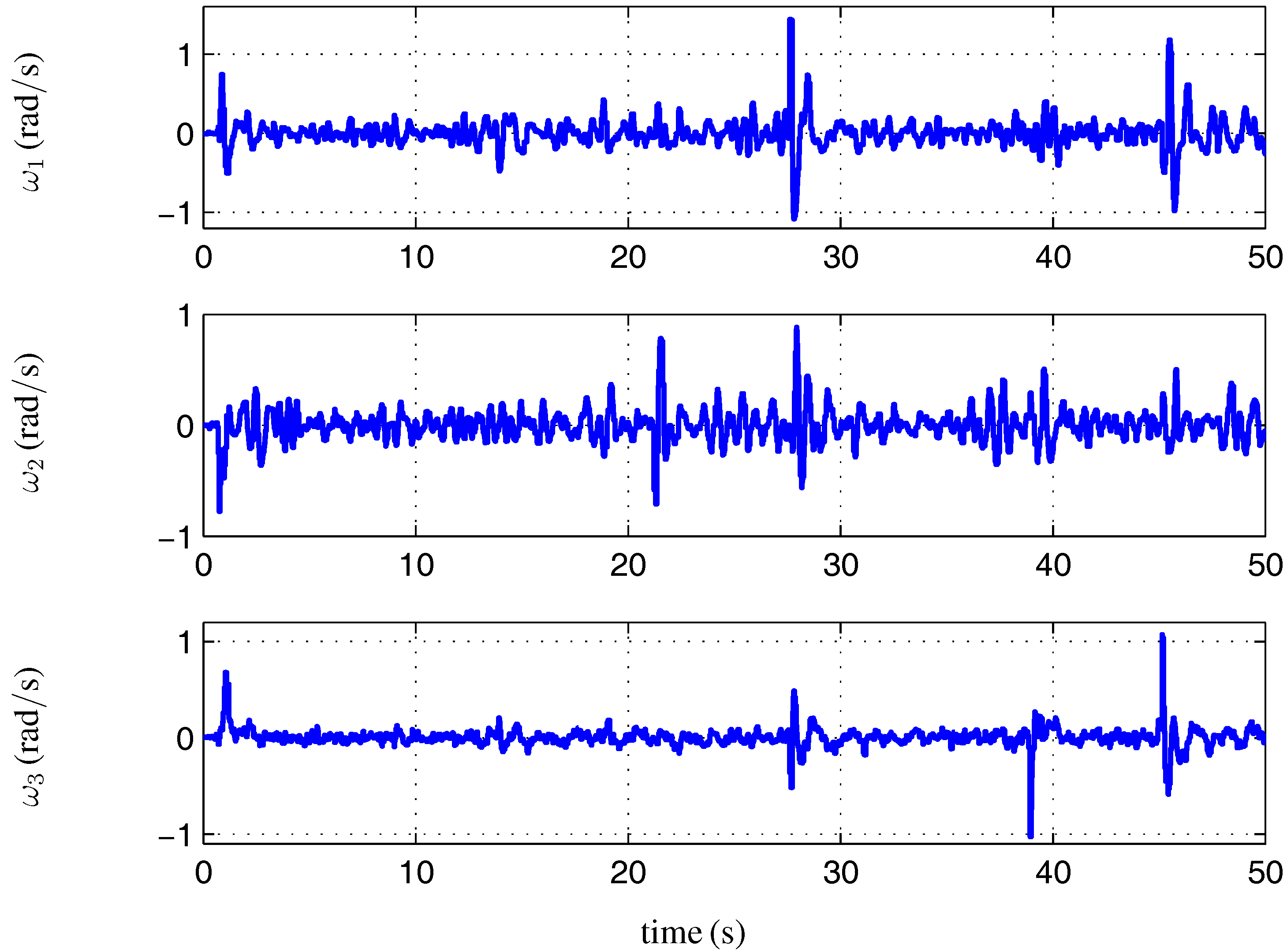
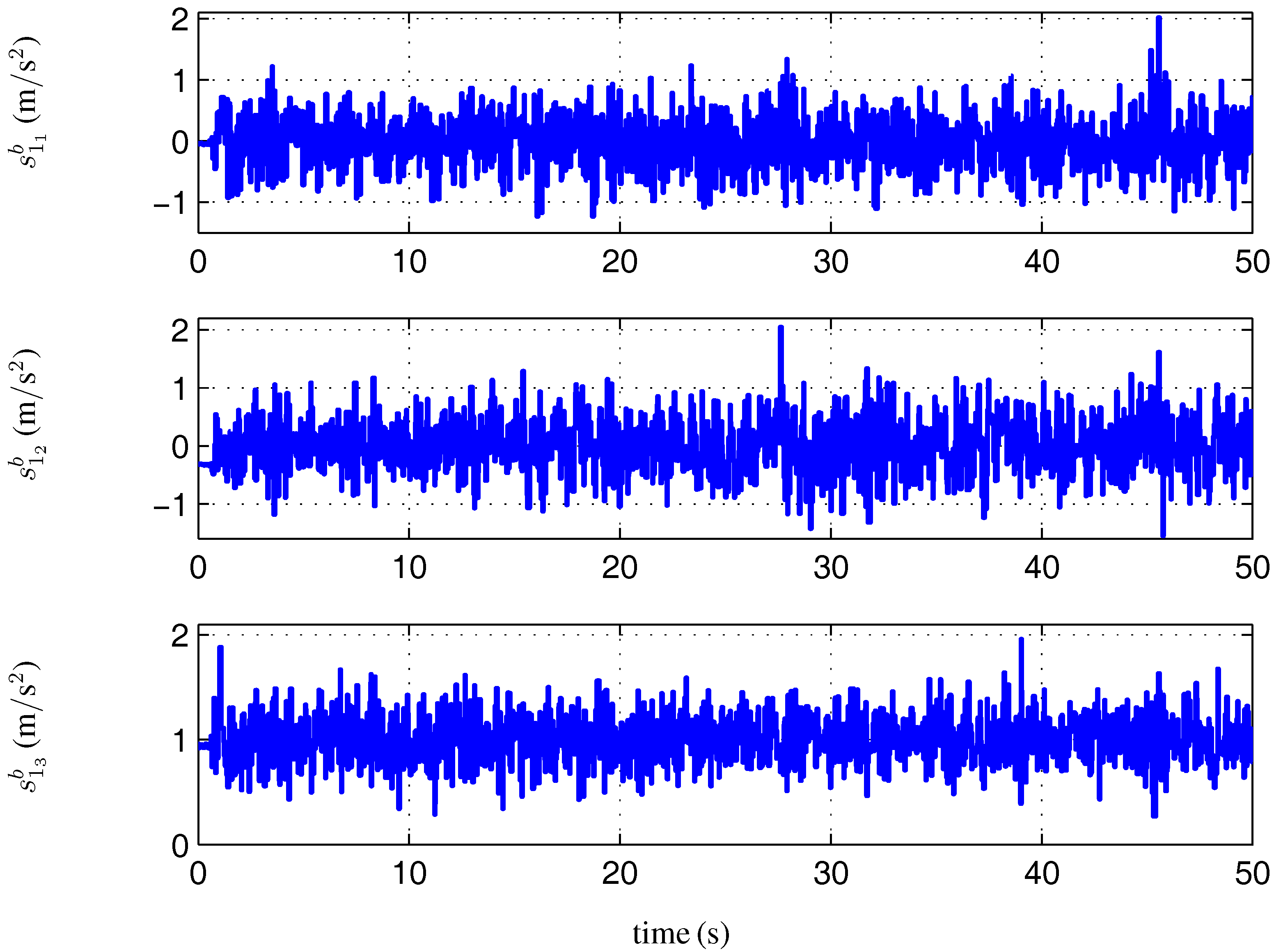
The tuning parameters of the control input are set to $N_{1,2}$ = 0.11, $N_3$ = 0.05, λ = 0.05 and ρ = 0.04. The initial conditions are $(\varphi$ = 18°, θ = −19° and ψ=−44°) for the roll, pitch and yaw angles, respectively, with a null angular velocity. The evolution of the the roll, pitch and yaw angles is shown in Figure 6. Note that the angles are not used to compute the control torque; they are presented only to show the attitude evolution, because they are more intuitive. The angular velocities, the vector observations (accelerometer and magnetometer measurements), the control torques and the pulse width of the motor control signals are presented in Figure 7, Figure 8, Figure 9, Figure 10 and Figure 11, respectively. The convergence of the angles and angular velocities is reached in an acceptable time (1.5 s). As can be seen in Figure 6 and Figure 7, the initial conditions produce a large error in the yaw angle and angular velocity. 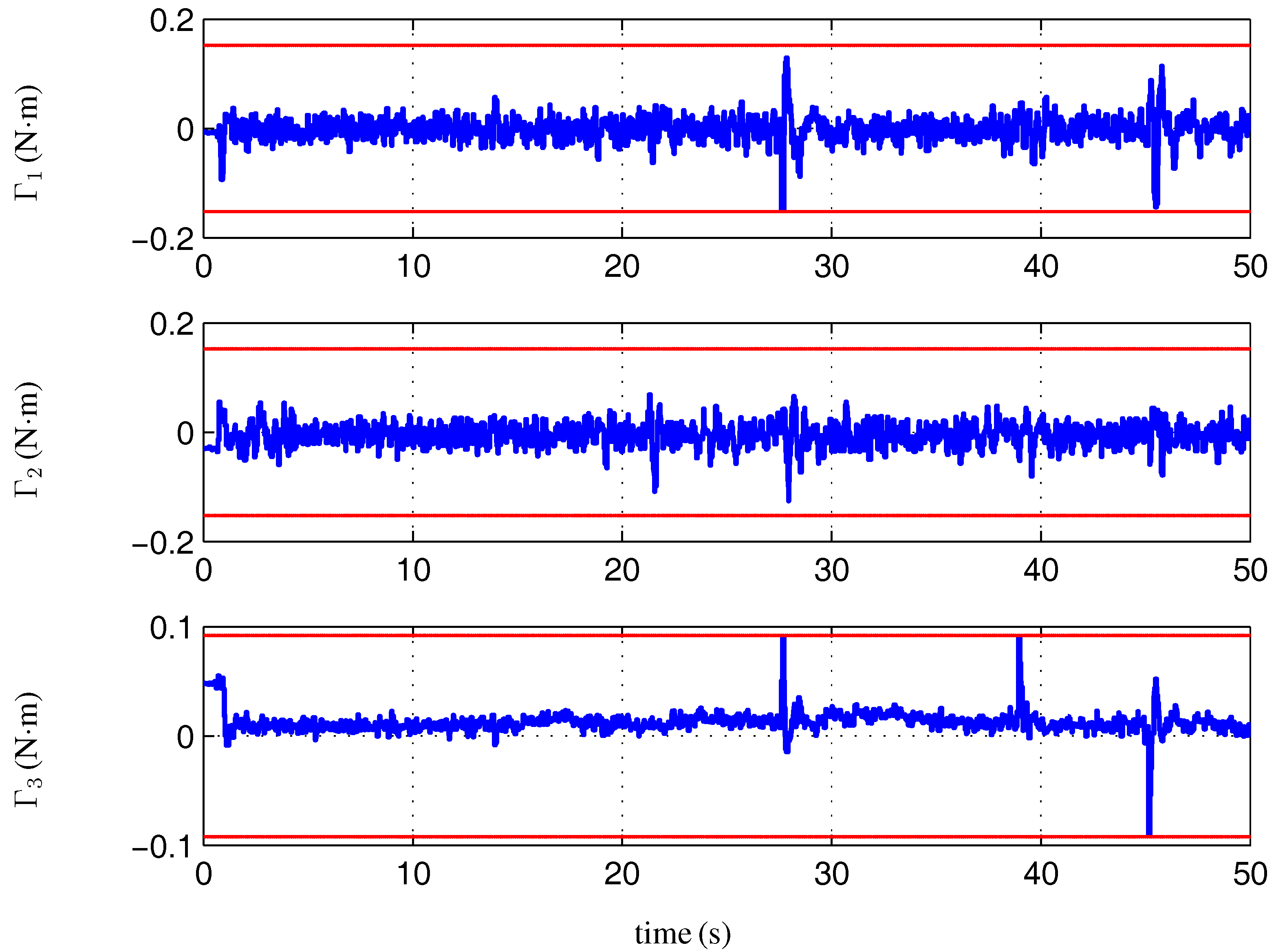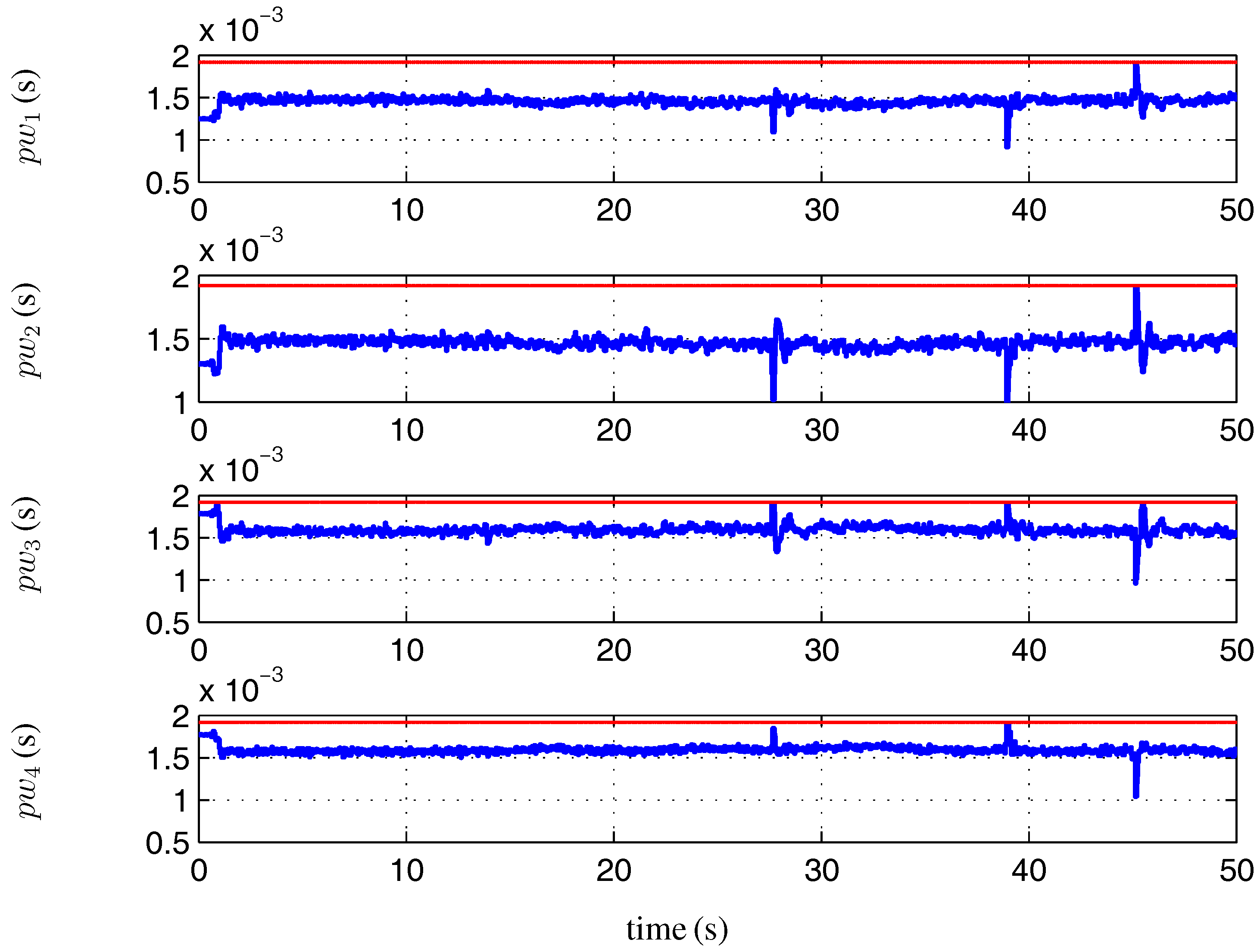Consequently, the control signal ${\mathrm{\Gamma }}_3$ reaches its bound of ±0.09 N·m (see Figure 10 and Figure 11) and takes action on the system to stabilize it. Note that there exists a slight deviation of the yaw angle. This is principally due to the disturbance in the magnetic field induced by the motors. In spite of the aforementioned deviations, the system behavior remains very acceptable.

The control law of Corollary 1 is also tested in the presence of disturbances applied successively to the three axes (roll, pitch and yaw). These disturbances can characterize some winds facing the engine. During experiments, the disturbances have been applied manually as a flick on the quadrotor body for less than one second. Note that the disturbance produces a large error of the yaw angle and the corresponding angular velocity, the control signal Γ₃ reaches its bound once more. Evidently, the control acts to bring the quadrotor to the desired attitude while respecting the motor constraints.

Figure 6. Control law of Corollary 1: the evolution of the roll, pitch and yaw angles.

Figure 6. Control law of Corollary 1: the evolution of the roll, pitch and yaw angles.

Figure 7. Control law of Corollary 1: the evolution of the body’s angular velocity.

Figure 7. Control law of Corollary 1: the evolution of the body’s angular velocity.

Figure 8. Control law of Corollary 1: the evolution of the accelerometer measurement $s_1^b$.

Figure 8. Control law of Corollary 1: the evolution of the accelerometer measurement $s_1^b$.

Figure 9. Control law of Corollary 1: the evolution of the magnetometer measurement $s_2^b$.

Figure 9. Control law of Corollary 1: the evolution of the magnetometer measurement $s_2^b$.

Figure 10. The bounded control torques of Corollary 1. The red dashed lines define the bounds of the control torques.

Figure 10. The bounded control torques of Corollary 1. The red dashed lines define the bounds of the control torques.

Figure 11. Control law of Corollary 1: the pulse width of the four motors’ control signals. The red dashed lines define the bounds of the pulse width.

Figure 11. Control law of Corollary 1: the pulse width of the four motors’ control signals. The red dashed lines define the bounds of the pulse width.

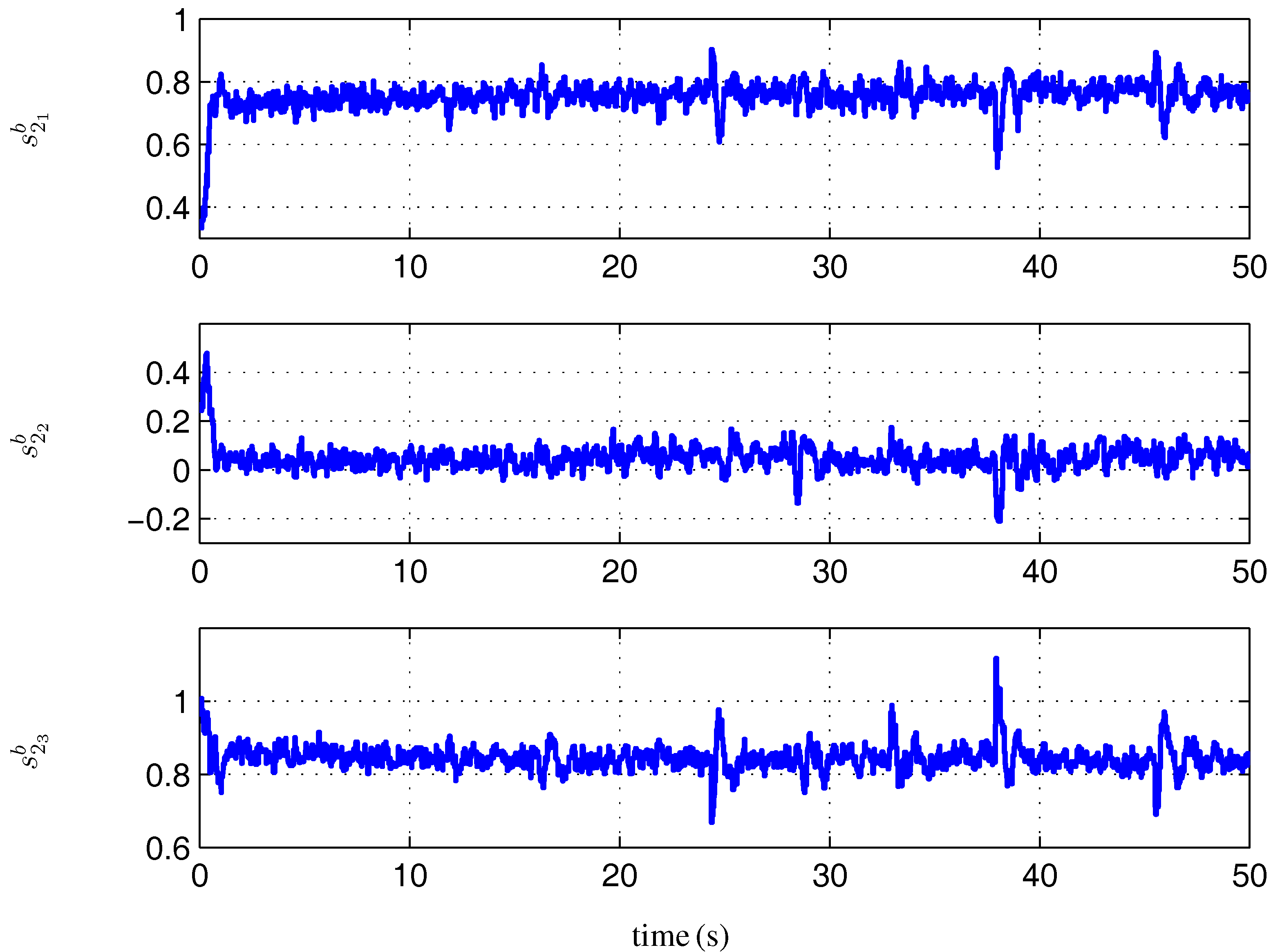
6.2. Stabilization Using the Control Law of Corollary 2

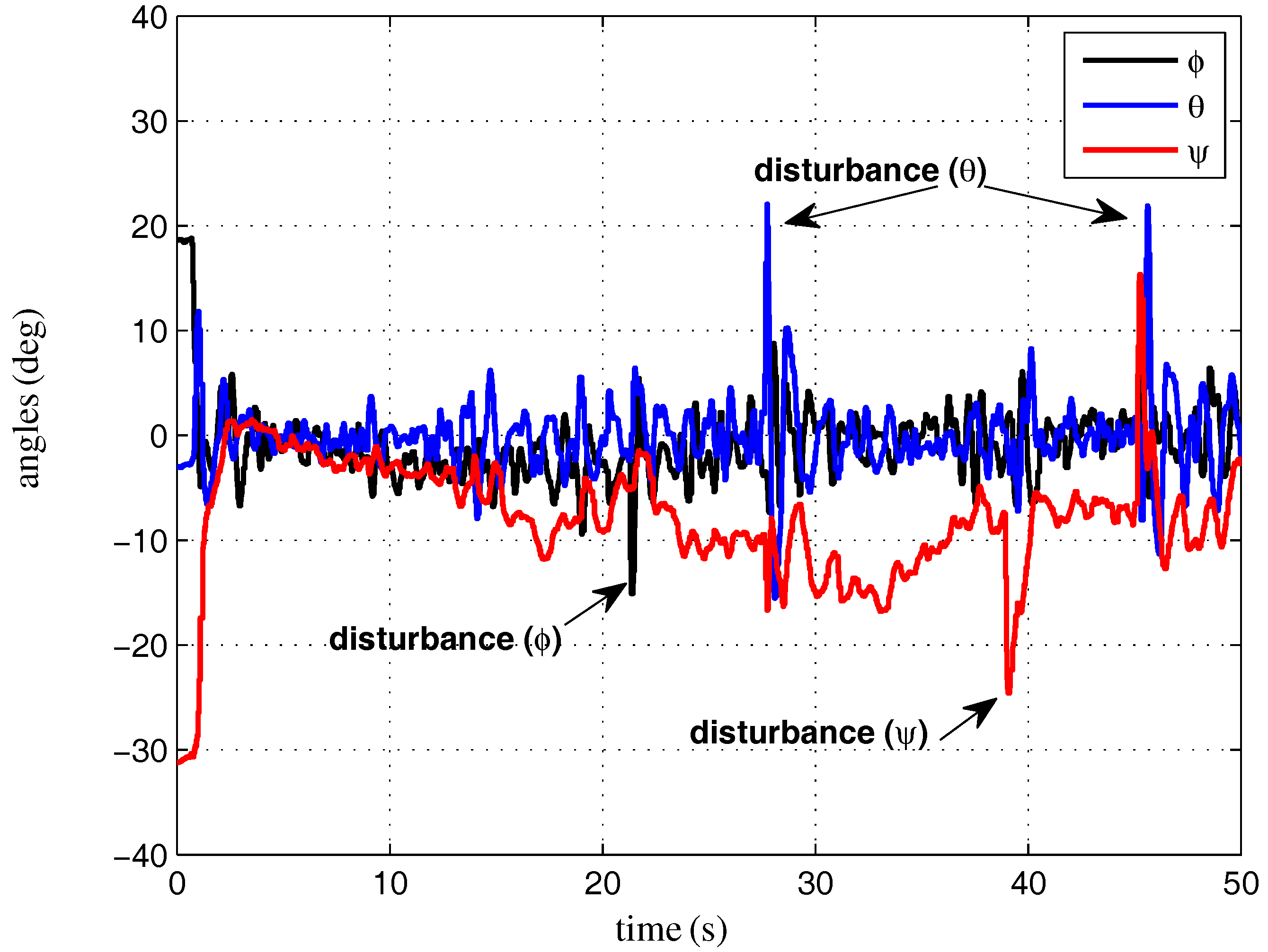
The control law presented in Corollary 2 is applied. The tuning parameters of the control input are set to ${\overline{N}}_{1,2}$ = 0.29, ${\overline{N}}_3$ = 0.866, λ = 0.06, ρ = 0.04, a = 25 and b = 5, in order to respect the constraint (20). The initial conditions are (ϕ = 19°, θ = −4° and ψ = −31°) for the roll, pitch and yaw angles, respectively, with a null angular velocity. One should be careful with setting the initial condition of the two last Equations of (16). A simple way is to set $\zeta (0)=v_m(0)-b{S}^b(0)$, when $v_m(0)=0$. 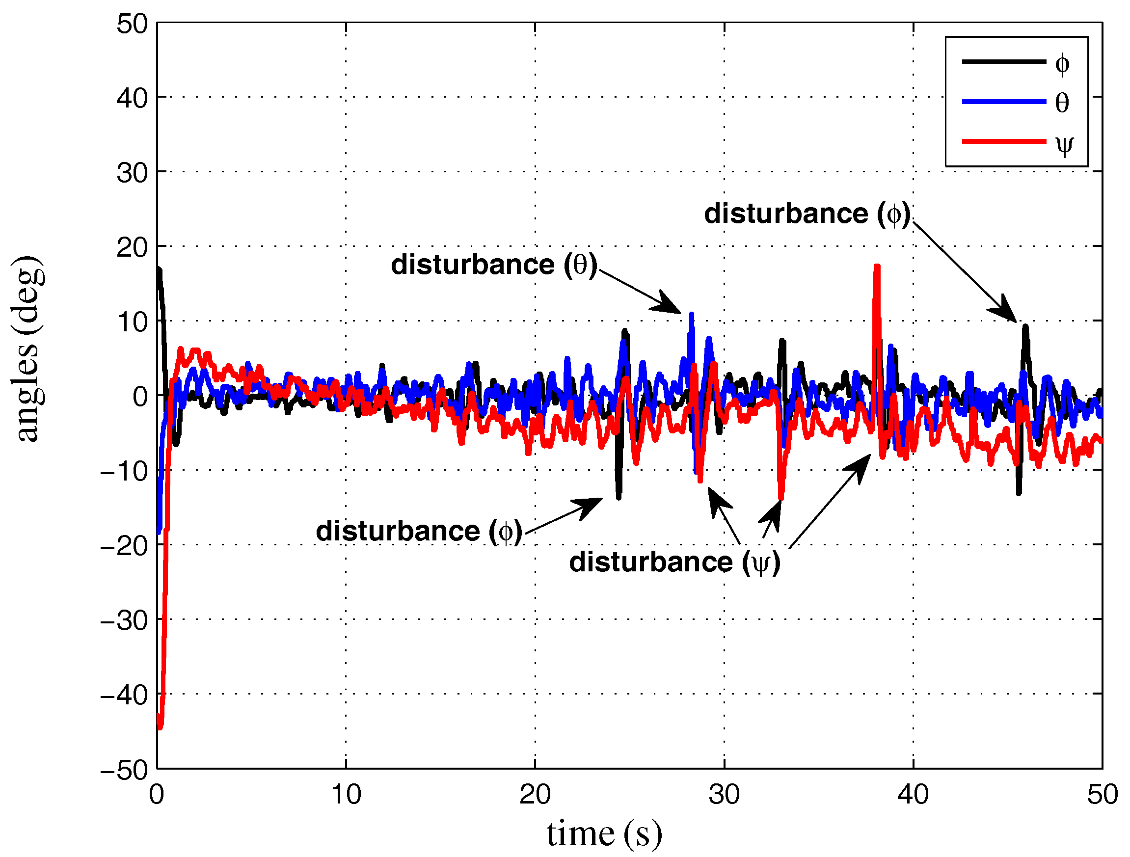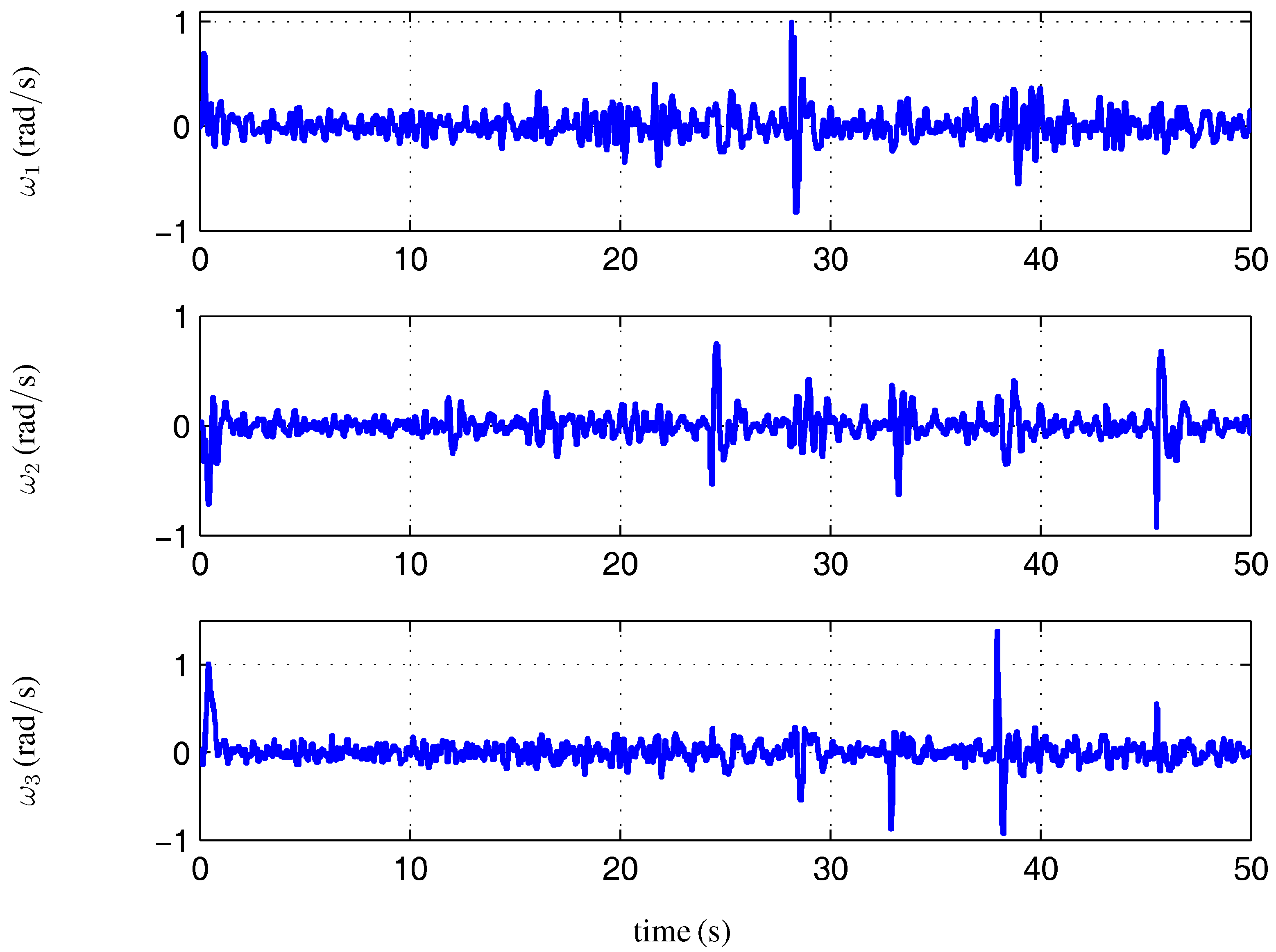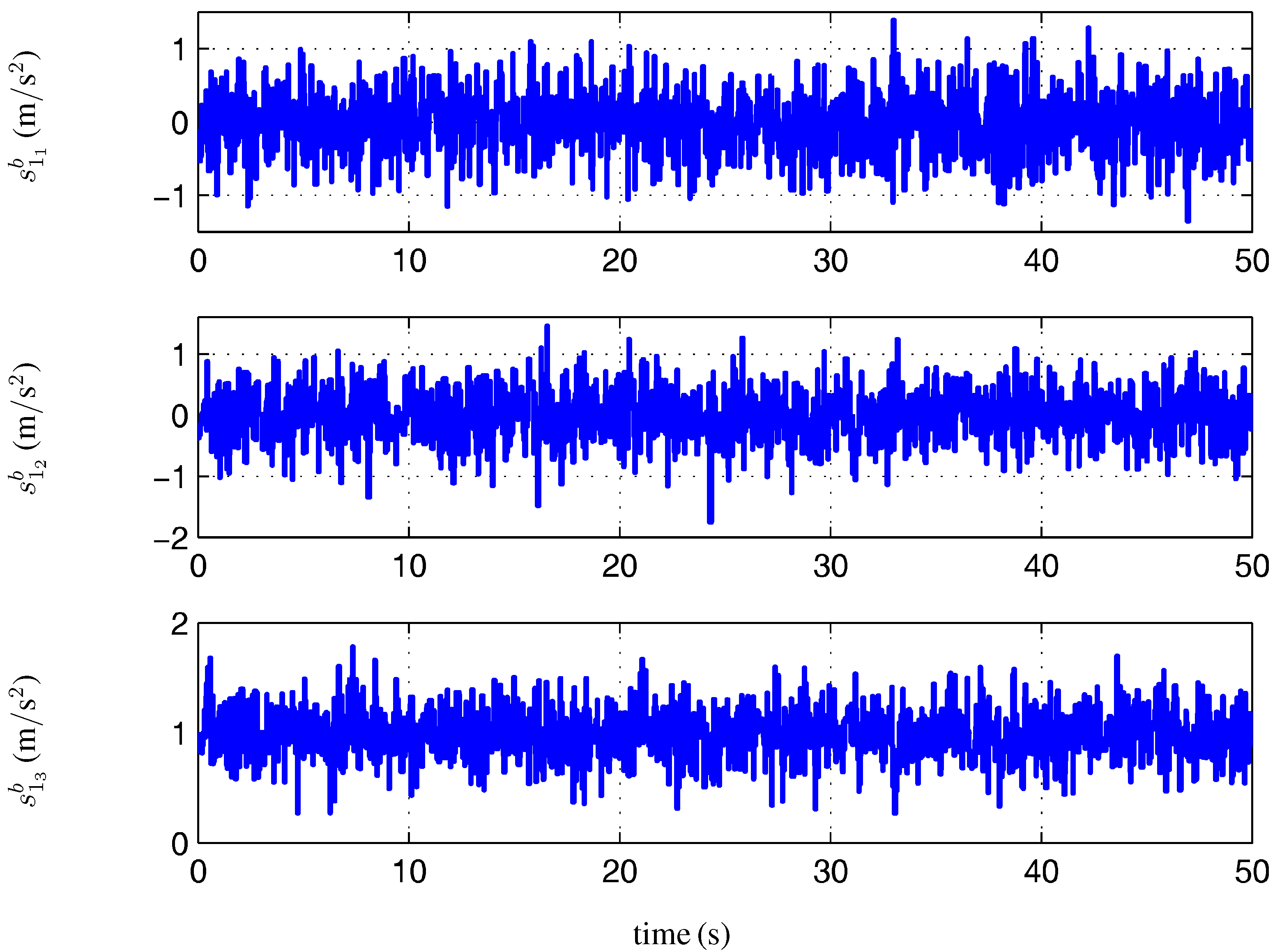The evolution of the the roll, pitch and yaw angles, the corresponding angular velocities, the vector observations (accelerometer and magnetometer measurements), the control torques and the pulse width of the motor control signals are presented, respectively, in Figure 12, Figure 13, Figure 14, Figure 15, Figure 16 and Figure 17. The convergence of the angles is reached in a suitable time (1.5 s). The variations of the control torque signals are more pronounced relative to the control law of Corollary 1. This is due to the disturbances induced by the vector observations used to reconstruct the angular velocity. Note that the vector observations are noisier than the rate gyros. However, the effect of oscillations is reduced when applied to the quadrotor, because the control signal is filtered by the motors. This can be explained by the fact that a DC motor is equivalent to an integrator that behaves as a low-pass filter or an averaging filter. As for the angles, the evolution of the angular velocity is depicted only for the sake of clarity. It is not used in the control law’s computation.

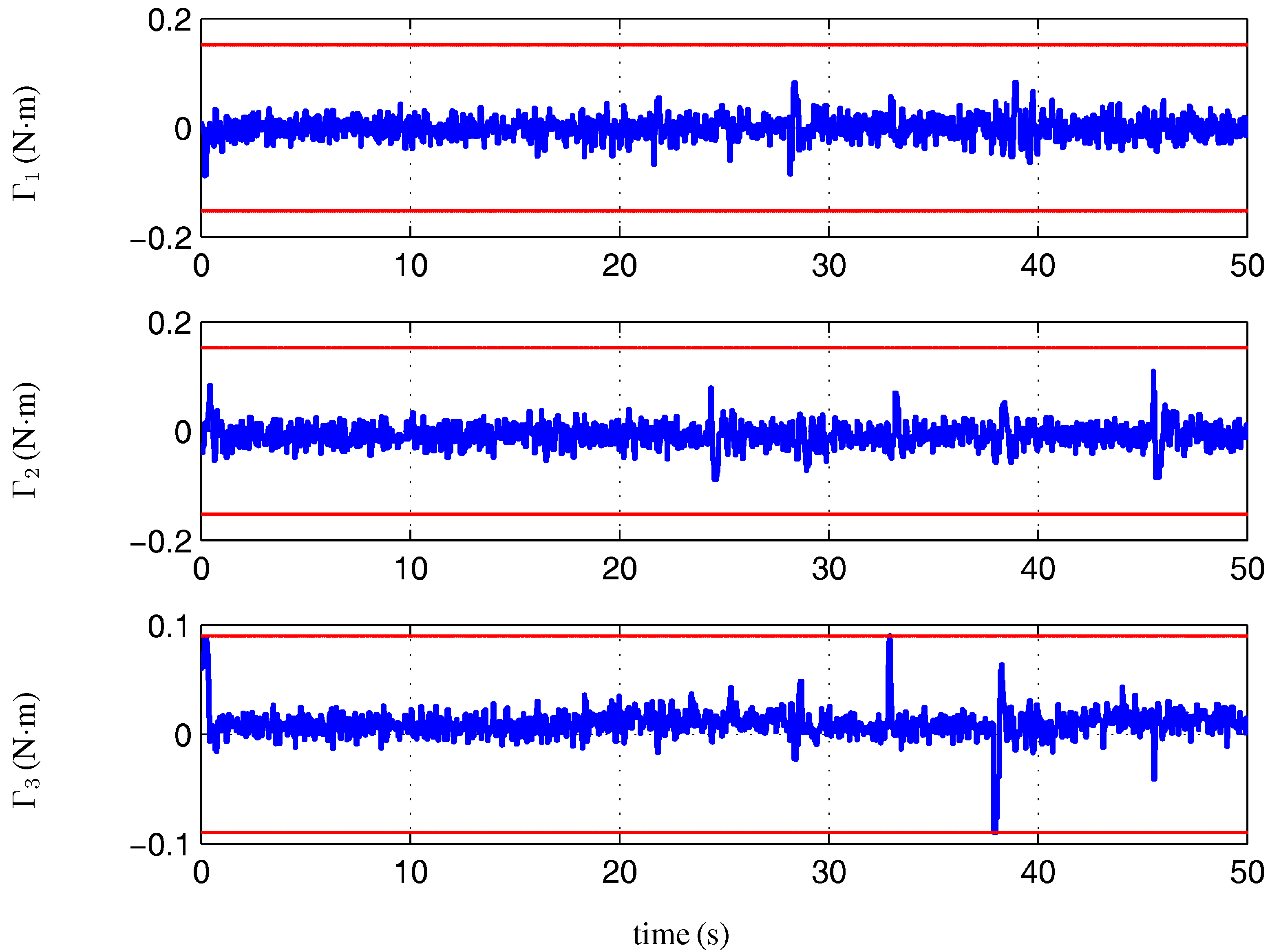
The present control law is tested with respect to some disturbances. Note that the disturbance produces a large error in the angles, as well as in the angular velocity, making the control signals ${\mathrm{\Gamma }}_1$ and ${\mathrm{\Gamma }}_3$ reach their bounds. Evidently, the control takes action on the system to overcome the disturbances, while only feasible control signals are applied to the system. This case study shows that the controller proposed in this paper is robust with respect to external disturbances. The control law maximizes the effectiveness of the actuators without endangering the system’s stability. This robustness property is essential in real missions, where aerodynamic forces and other factors are present.

Figure 12. Control law of Corollary 2: the evolution of the roll, pitch and yaw angles.

Figure 12. Control law of Corollary 2: the evolution of the roll, pitch and yaw angles.

Figure 13. Control law of Corollary 2: the evolution of the body’s angular velocity.

Figure 13. Control law of Corollary 2: the evolution of the body’s angular velocity.

Figure 14. Control law of Corollary 2: the evolution of the accelerometer measurement $s_1^b$.

Figure 14. Control law of Corollary 2: the evolution of the accelerometer measurement $s_1^b$.

Figure 15. Control law of Corollary 2: the evolution of the magnetometer measurement $s_2^b$.

Figure 15. Control law of Corollary 2: the evolution of the magnetometer measurement $s_2^b$.

Figure 16. The bounded control torques of Corollary 2. The red dashed lines define the bounds of the control torques.

Figure 16. The bounded control torques of Corollary 2. The red dashed lines define the bounds of the control torques.

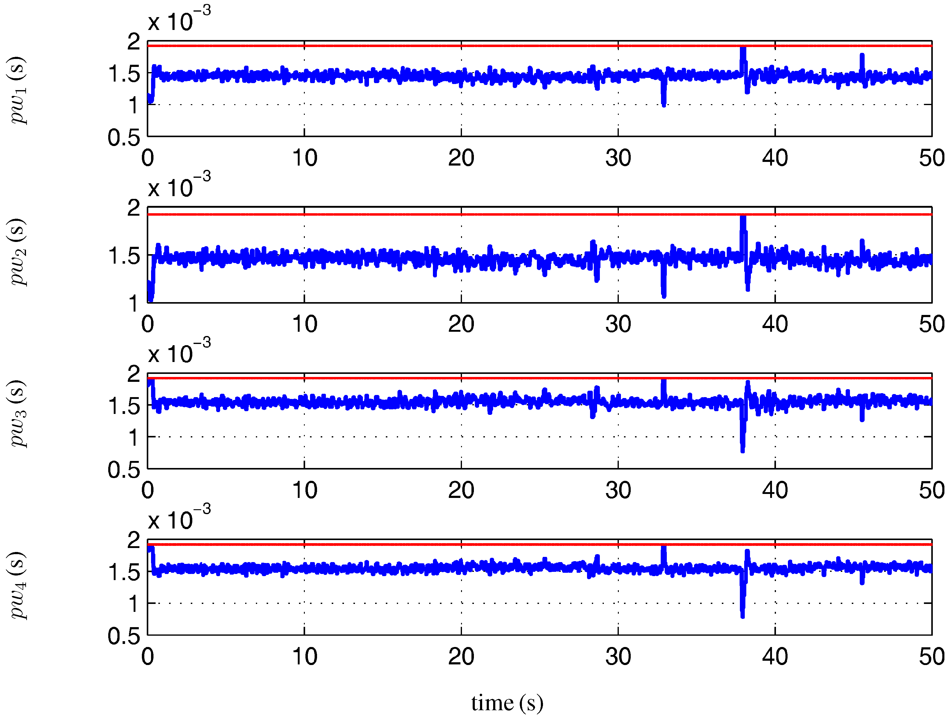
Figure 17. Control law of Corollary 2: the pulse width of the four motors’ control signals. The red dashed lines define the bounds of the pulse width.

Figure 17. Control law of Corollary 2: the pulse width of the four motors’ control signals. The red dashed lines define the bounds of the pulse width.

7. Conclusions

A biomimetic-based approach, inspired by insect flight, is presented in this paper for stabilizing rigid bodies. This approach is based on the direct measurements of embedded sensors that mimic some sensitive organs of flapping flyers, such as halteres, leg sensilla and magnetic sense. The boundedness of the developed torques is also taken into account in this strategy. In other words, two bounded stabilizing control torques based on a bounded feedback and computed over direct sensor measurements are proposed. The first one is based on a rate gyro and directional sensor measurements. The second one spares the angular velocity measurement and uses only directional sensor measurements. These biomimetic-based control laws are low cost in terms of computations, since they take into account the saturation of the actuators, are independent of the body’s inertia, ensure the asymptotic stability of the system and do not need an explicit attitude reconstruction. The stability of the closed loop system, subjected to the control laws, is proven by means of Lyapunov analyses. Note that the proof is not limited to symmetric bodies, like quadrotor UAVs. The proof is therefore valid for possibly non-symmetric rigid bodies. In spite of the sensor measurement disturbances, the stability of the proposed biomimetic-based control laws is validated in real time through experimental tests using the quadrotor UAV of the Autonomous University of Puebla (BUAP). Their robustness with respect to external disturbances is also shown.

Future work concerns the application of this approach in real time on the flapping wing micro-aerial vehicle prototype developed in the context of the project “Cooperative Control of Micro-UAVs for Mapping and Precision Agriculture” supported by the Research and Postgraduate Office of the Autonomous University of Puebla (VIEP-BUAP).