
Deep Learning Approaches to Osteosarcoma Diagnosis and Classification: A Comparative Methodological Approach


Simple Summary
Abstract
1. Introduction
2. Methodology
2.1. Methodological Description of Deep Learning Methodologies
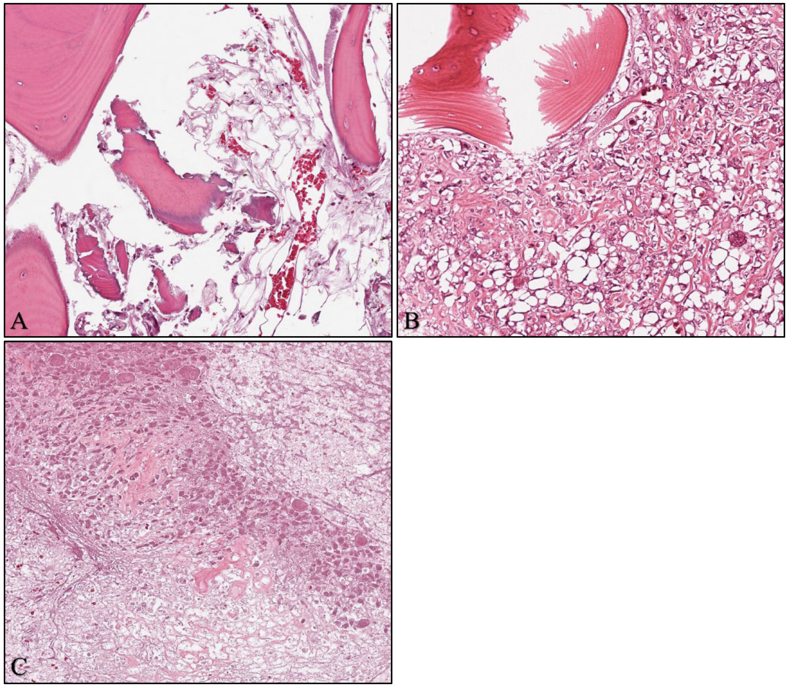
2.2. Dataset
2.3. Experimental Setup
2.4. Network Evaluation
2.5. Follow-Up Experiment
3. Results
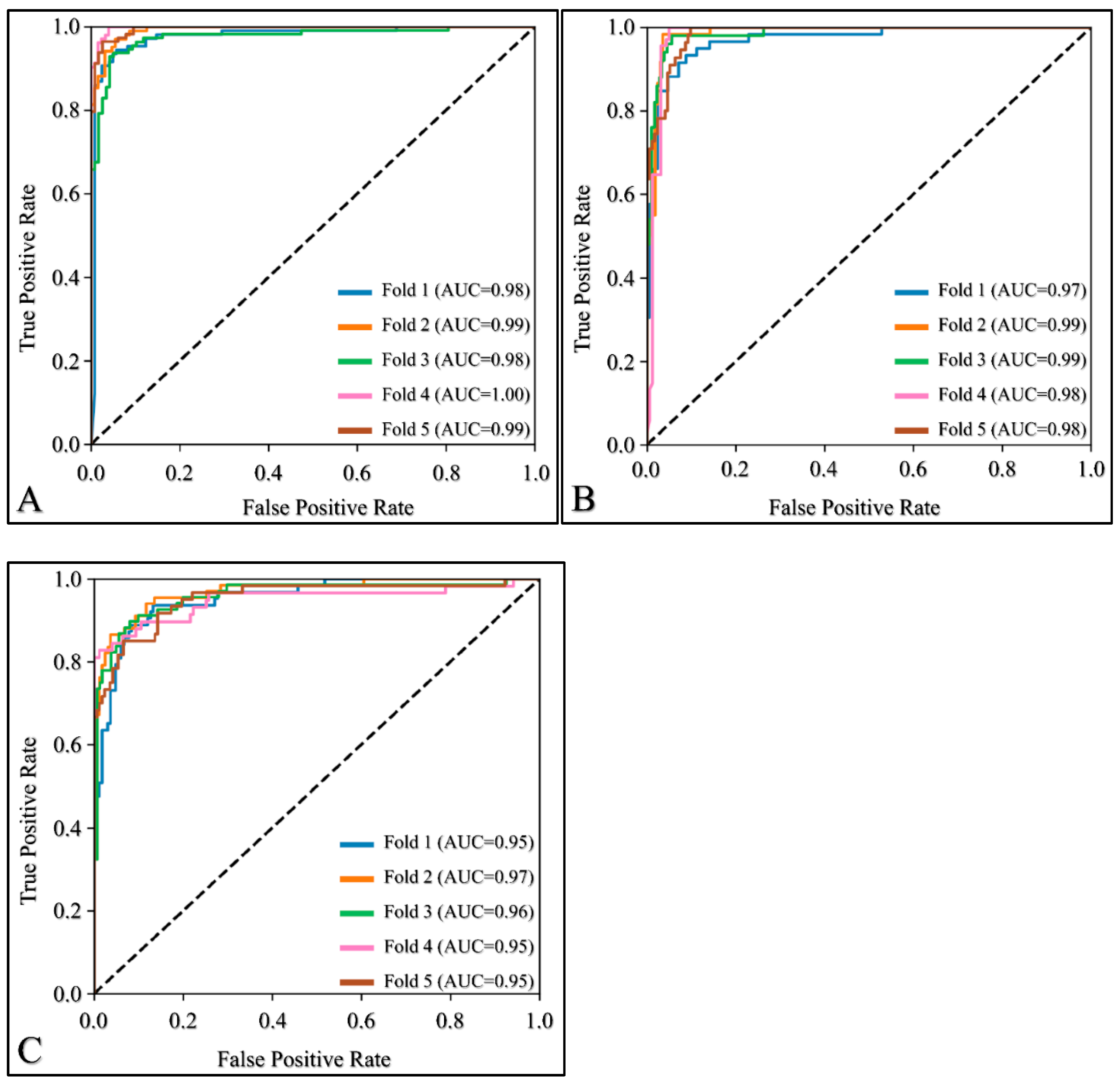
3.1. Network Comparison
3.2. Follow-Up Experiment
4. Discussion
4.1. Comparing Neural Networks

| Study | Method | Validation Strategy | Overall Accuracy |
|---|---|---|---|
| Arunachalam et al. (2019) [35] | Custom CNN | Holdout | 0.910 |
| Anisuzzaman et al. (2021) [53] | VGG19 | Holdout | 0.940 |
| Bansal et al. (2022) [59] | Combination of HC and DL features | Holdout | 0.995 |
| Present study | MobileNetV2 | Cross-Validation | 0.910 |
4.2. Limitations and Future Perspectives
5. Conclusions
Supplementary Materials
Author Contributions
Funding
Institutional Review Board Statement
Informed Consent Statement
Data Availability Statement
Conflicts of Interest
References
- Luetke, A.; Meyers, P.A.; Lewis, I.; Juergens, H. Osteosarcoma treatment—Where do we stand? A state of the art review. Cancer Treat. Rev. 2014, 40, 523–532. [Google Scholar] [CrossRef] [PubMed]
- Koutsomplia, G.; Lambrou, G.I. Resistance mechanisms in the radiation therapy of osteosarcoma: A brief review. J. Res. Pract. Musculoskelet. Syst. 2020, 4, 15–19. [Google Scholar] [CrossRef][Green Version]
- Thomas, N.A.; Abraham, R.G.; Dedi, B.; Krucher, N.A. Targeting retinoblastoma protein phosphorylation in combination with egfr inhibition in pancreatic cancer cells. Int. J. Oncol. 2019, 54, 527–536. [Google Scholar]
- Matlashewski, G.; Lamb, P.; Pim, D.; Peacock, J.; Crawford, L.; Benchimol, S. Isolation and characterization of a human p53 cdna clone: Expression of the human p53 gene. EMBO J. 1984, 3, 3257–3262. [Google Scholar] [CrossRef] [PubMed]
- Chen, W.; Liu, Q.; Fu, B.; Liu, K.; Jiang, W. Overexpression of grim-19 accelerates radiation-induced osteosarcoma cells apoptosis by p53 stabilization. Life Sci. 2018, 208, 232–238. [Google Scholar] [CrossRef] [PubMed]
- Lambrou, G.I.; Vlahopoulos, S.; Papathanasiou, C.; Papanikolaou, M.; Karpusas, M.; Zoumakis, E.; Tzortzatou-Stathopoulou, F. Prednisolone exerts late mitogenic and biphasic effects on resistant acute lymphoblastic leukemia cells: Relation to early gene expression. Leuk. Res. 2009, 33, 1684–1695. [Google Scholar] [CrossRef]
- Miller, A.C.; Kariko, K.; Myers, C.E.; Clark, E.P.; Samid, D. Increased radioresistance of ejras-transformed human osteosarcoma cells and its modulation by lovastatin, an inhibitor of p21ras isoprenylation. Int. J. Cancer 1993, 53, 302–307. [Google Scholar] [CrossRef]
- Miller, A.C.; Gafner, J.; Clark, E.P.; Samid, D. Differences in radiation-induced micronuclei yields of human cells: Influence of ras gene expression and protein localization. Int. J. Radiat. Biol. 1993, 64, 547–554. [Google Scholar] [CrossRef]
- Campbell, K.J.; Chapman, N.R.; Perkins, N.D. Uv stimulation induces nuclear factor kappab (nf-kappab) DNA-binding activity but not transcriptional activation. Biochem. Soc. Trans. 2001, 29, 688–691. [Google Scholar] [CrossRef]
- Chaussade, A.; Millot, G.; Wells, C.; Brisse, H.; Lae, M.; Savignoni, A.; Desjardins, L.; Dendale, R.; Doz, F.; Aerts, I.; et al. Correlation between rb1germline mutations and second primary malignancies in hereditary retinoblastoma patients treated with external beam radiotherapy. Eur. J. Med. Genet. 2019, 62, 217–223. [Google Scholar] [CrossRef]
- Surget, S.; Khoury, M.P.; Bourdon, J.C. Uncovering the role of p53 splice variants in human malignancy: A clinical perspective. OncoTargets Ther. 2013, 7, 57–68. [Google Scholar]
- Park, D.E.; Cheng, J.; Berrios, C.; Montero, J.; Cortes-Cros, M.; Ferretti, S.; Arora, R.; Tillgren, M.L.; Gokhale, P.C.; DeCaprio, J.A. Dual inhibition of mdm2 and mdm4 in virus-positive merkel cell carcinoma enhances the p53 response. Proc. Natl. Acad. Sci. USA 2019, 116, 1027–1032. [Google Scholar] [CrossRef]
- Gilmore, T.D. Introduction to nf-kappab: Players, pathways, perspectives. Oncogene 2006, 25, 6680–6684. [Google Scholar] [CrossRef] [PubMed]
- Taniguchi, K.; Karin, M. Nf-kappab, inflammation, immunity and cancer: Coming of age. Nat. Rev. Immunol. 2018, 18, 309–324. [Google Scholar] [CrossRef]
- Vlahopoulos, S.A.; Cen, O.; Hengen, N.; Agan, J.; Moschovi, M.; Critselis, E.; Adamaki, M.; Bacopoulou, F.; Copland, J.A.; Boldogh, I.; et al. Dynamic aberrant nf-kappab spurs tumorigenesis: A new model encompassing the microenvironment. Cytokine Growth Factor Rev. 2015, 26, 389–403. [Google Scholar] [CrossRef]
- Nouri, M.; Massah, S.; Caradec, J.; Lubik, A.A.; Li, N.; Truong, S.; Lee, A.R.; Fazli, L.; Ramnarine, V.R.; Lovnicki, J.M.; et al. Transient sox9 expression facilitates resistance to androgen-targeted therapy in prostate cancer. Clin Cancer Res 2020, 26, 1678–1689. [Google Scholar] [CrossRef] [PubMed]
- Zhang, B.; Shi, Z.L.; Liu, B.; Yan, X.B.; Feng, J.; Tao, H.M. Enhanced anticancer effect of gemcitabine by genistein in osteosarcoma: The role of akt and nuclear factor-kappab. Anti-Cancer Drugs 2010, 21, 288–296. [Google Scholar] [CrossRef]
- Tsagaraki, I.; Tsilibary, E.C.; Tzinia, A.K. Timp-1 interaction with alphavbeta3 integrin confers resistance to human osteosarcoma cell line mg-63 against tnf-alpha-induced apoptosis. Cell Tissue Res. 2010, 342, 87–96. [Google Scholar] [CrossRef] [PubMed]
- Li, K.; Li, X.; Tian, J.; Wang, H.; Pan, J.; Li, J. Downregulation of DNA-pkcs suppresses p-gp expression via inhibition of the akt/nf-kappab pathway in cd133-positive osteosarcoma mg-63 cells. Oncol. Rep. 2016, 36, 1973–1980. [Google Scholar] [CrossRef]
- Yan, M.; Ni, J.; Song, D.; Ding, M.; Huang, J. Activation of unfolded protein response protects osteosarcoma cells from cisplatin-induced apoptosis through nf-kappab pathway. Int. J. Clin. Exp. Pathol. 2015, 8, 10204–10215. [Google Scholar]
- Taran, S.J.; Taran, R.; Malipatil, N.B. Pediatric osteosarcoma: An updated review. Indian J. Med. Paediatr. Oncol. 2017, 38, 33–43. [Google Scholar] [CrossRef] [PubMed]
- Siegel, R.L.; Miller, K.D.; Fuchs, H.E.; Jemal, A. Cancer statistics, 2022. CA Cancer J. Clin. 2022, 72, 7–33. [Google Scholar] [CrossRef] [PubMed]
- Smeland, S.; Bielack, S.S.; Whelan, J.; Bernstein, M.; Hogendoorn, P.; Krailo, M.D.; Gorlick, R.; Janeway, K.A.; Ingleby, F.C.; Anninga, J.; et al. Survival and prognosis with osteosarcoma: Outcomes in more than 2000 patients in the euramos-1 (european and american osteosarcoma study) cohort. Eur. J. Cancer 2019, 109, 36–50. [Google Scholar] [CrossRef] [PubMed]
- Friebele, J.C.; Peck, J.; Pan, X.; Abdel-Rasoul, M.; Mayerson, J.L. Osteosarcoma: A meta-analysis and review of the literature. Am. J. Orthop. 2015, 44, 547–553. [Google Scholar]
- Jiang, Y.; Wang, X.; Cheng, Y.; Peng, J.; Xiao, J.; Tang, D.; Yi, Y. Associations between inflammatory gene polymorphisms (tnf-alpha 308g/a, tnf-alpha 238g/a, tnf-beta 252a/g, tgf-beta1 29t/c, il-6 174g/c and il-10 1082a/g) and susceptibility to osteosarcoma: A meta-analysis and literature review. Oncotarget 2017, 8, 97571–97583. [Google Scholar] [CrossRef]
- Bajpai, J.; Kumar, R.; Sreenivas, V.; Sharma, M.C.; Khan, S.A.; Rastogi, S.; Malhotra, A.; Gamnagatti, S.; Kumar, R.; Safaya, R.; et al. Prediction of chemotherapy response by pet-ct in osteosarcoma: Correlation with histologic necrosis. J. Pediatr. Hematol. Oncol. 2011, 33, e271–e278. [Google Scholar] [CrossRef]
- Emerson, J.L. Observer bias in histopathological examinations. In Carcinogenicity: The Design, Analysis, and Interpretation of Long-Term Animal Studies; Grice, H.C., Ciminera, J.L., Eds.; Springer: Berlin/Heidelberg, Germany, 1988; pp. 137–147. [Google Scholar]
- Asilian Bidgoli, A.; Rahnamayan, S.; Dehkharghanian, T.; Grami, A.; Tizhoosh, H.R. Bias reduction in representation of histopathology images using deep feature selection. Sci. Rep. 2022, 12, 19994. [Google Scholar] [CrossRef]
- Jeong, S.Y.; Kim, W.; Byun, B.H.; Kong, C.B.; Song, W.S.; Lim, I.; Lim, S.M.; Woo, S.K. Prediction of chemotherapy response of osteosarcoma using baseline (18)f-fdg textural features machine learning approaches with pca. Contrast Media Mol. Imaging 2019, 2019, 3515080. [Google Scholar] [CrossRef]
- Zhang, L.; Ge, Y.; Gao, Q.; Zhao, F.; Cheng, T.; Li, H.; Xia, Y. Machine learning-based radiomics nomogram with dynamic contrast-enhanced mri of the osteosarcoma for evaluation of efficacy of neoadjuvant chemotherapy. Front. Oncol. 2021, 11, 758921. [Google Scholar] [CrossRef]
- Buhnemann, C.; Li, S.; Yu, H.; Branford White, H.; Schafer, K.L.; Llombart-Bosch, A.; Machado, I.; Picci, P.; Hogendoorn, P.C.; Athanasou, N.A.; et al. Quantification of the heterogeneity of prognostic cellular biomarkers in ewing sarcoma using automated image and random survival forest analysis. PLoS ONE 2014, 9, e107105. [Google Scholar] [CrossRef]
- Essa, E.; Xie, X.; Errington, R.J.; White, N. A multi-stage random forest classifier for phase contrast cell segmentation. In Proceedings of the In 2015 37th Annual International Conference of the IEEE Engineering in Medicine and Biology Society, Milan, Italy, 25–29 August 2015; pp. 3865–3868. [Google Scholar]
- Li, W.; Dong, Y.; Liu, W.; Tang, Z.; Sun, C.; Lowe, S.; Chen, S.; Bentley, R.; Zhou, Q.; Xu, C.; et al. A deep belief network-based clinical decision system for patients with osteosarcoma. Front. Immunol. 2022, 13, 1003347. [Google Scholar] [CrossRef]
- Shen, R.; Li, Z.; Zhang, L.; Hua, Y.; Mao, M.; Li, Z.; Cai, Z.; Qiu, Y.; Gryak, J.; Najarian, K. Osteosarcoma patients classification using plain x-rays and metabolomic data. In Proceedings of the 2018 40th Annual International Conference of the IEEE Engineering in Medicine and Biology Society (EMBC), Honolulu, HI, USA, 18–21 July 2018; pp. 690–693. [Google Scholar]
- Arunachalam, H.B.; Mishra, R.; Daescu, O.; Cederberg, K.; Rakheja, D.; Sengupta, A.; Leonard, D.; Hallac, R.; Leavey, P. Viable and necrotic tumor assessment from whole slide images of osteosarcoma using machine-learning and deep-learning models. PLoS ONE 2019, 14, e0210706. [Google Scholar] [CrossRef] [PubMed]
- Komura, D.; Ishikawa, S. Machine learning methods for histopathological image analysis. Comput. Struct. Biotechnol. J. 2018, 16, 34–42. [Google Scholar] [CrossRef]
- Melanthota, S.K.; Gopal, D.; Chakrabarti, S.; Kashyap, A.A.; Radhakrishnan, R.; Mazumder, N. Deep learning-based image processing in optical microscopy. Biophys. Rev. 2022, 14, 463–481. [Google Scholar] [CrossRef]
- Ong, S.H.; Jin, X.C.; Jayasooriah; Sinniah, R. Image analysis of tissue sections. Comput. Biol. Med. 1996, 26, 269–279. [Google Scholar] [CrossRef] [PubMed]
- Shin, H.C.; Roth, H.R.; Gao, M.; Lu, L.; Xu, Z.; Nogues, I.; Yao, J.; Mollura, D.; Summers, R.M. Deep convolutional neural networks for computer-aided detection: Cnn architectures, dataset characteristics and transfer learning. IEEE Trans. Med. Imaging 2016, 35, 1285–1298. [Google Scholar] [CrossRef]
- Deng, J.; Dong, W.; Socher, R.; Li, L.J.; Kai, L.; Li, F.-F. Imagenet: A large-scale hierarchical image database. In Proceedings of the 2009 IEEE Conference on Computer Vision and Pattern Recognition, Miami, FL, USA, 20–25 June 2009; pp. 248–255. [Google Scholar]
- Krizhevsky, A.; Sutskever, I.; Hinton, G.E. Imagenet classification with deep convolutional neural networks. Commun. ACM 2017, 60, 84–90. [Google Scholar] [CrossRef]
- Wang, F.; Oh, T.W.; Vergara-Niedermayr, C.; Kurc, T.; Saltz, J. Managing and querying whole slide images. Proc. SPIE—Int. Soc. Opt. Eng. 2012, 8319, 137–148. [Google Scholar]
- Leavey, P.; Sengupta, A.; Rakheja, D.; Daescu, O.; Arunachalam, H.B.; Mishra, R. Osteosarcoma data from ut southwestern/ut dallas for viable and necrotic tumor assessment [data set]. Cancer Imaging Arch. 2019, 14. [Google Scholar] [CrossRef]
- Mishra, R.; Daescu, O.; Leavey, P.; Rakheja, D.; Sengupta, A. Histopathological Diagnosis for Viable and Non-Viable Tumor Prediction for Osteosarcoma Using Convolutional Neural Network; Springer International Publishing: Cham, Switzerland, 2017; pp. 12–23. [Google Scholar]
- Arunachalam, H.B.; Mishra, R.; Armaselu, B.; Daescu, O.; Martinez, M.; Leavey, P.; Rakheja, D.; Cederberg, K.; Sengupta, A.; Ni’suilleabhain, M. Computer aided image segmentation and classification for viable and non-viable tumor identification in osteosarcoma. Pac. Symp. Biocomput. 2017, 22, 195–206. [Google Scholar]
- Mishra, R.; Daescu, O.; Leavey, P.; Rakheja, D.; Sengupta, A. Convolutional neural network for histopathological analysis of osteosarcoma. J. Comput. Biol. 2018, 25, 313–325. [Google Scholar] [CrossRef]
- Leavey, P.; Arunachalam, H.B.; Armaselu, B.; Sengupta, A.; Rakheja, D.; Skapek, S.; Cederberg, K.; Bach, J.-P.; Glick, S.; Ni’Suilleabhain, M. Implementation of Computer-Based Image Pattern Recognition Algorithms to Interpret Tumor Necrosis; A First Step in Development of a Novel Biomarker in Osteosarcoma; Pediatric Blood & Cancer; Wiley: Hoboken, NJ, USA, 2017; p. S52. [Google Scholar]
- Simonyan, K.; Zisserman, A. Very deep convolutional networks for large-scale image recognition. arXiv 2015, arXiv:1409.1556. [Google Scholar]
- He, K.; Zhang, X.; Ren, S.; Sun, J. Deep residual learning for image recognition. arXiv 2015, arXiv:1512.03385. [Google Scholar]
- Howard, A.G.; Zhu, M.; Chen, B.; Kalenichenko, D.; Wang, W.; Weyand, T.; Andreetto, M.; Adam, H. Mobilenets: Efficient convolutional neural networks for mobile vision applications. arXiv 2017, arXiv:1704.04861. [Google Scholar]
- Tan, M.; Le, Q.V. Efficientnet: Rethinking model scaling for convolutional neural networks. In Proceedings of the 36th International Conference on Machine Learning, Long Beach, CA, USA, 9–15 June 2019; Chaudhuri, K., Salakhutdinov, R., Eds.; Volume 97, pp. 6105–6114. [Google Scholar]
- Dosovitskiy, A.; Beyer, L.; Kolesnikov, A.; Weissenborn, D.; Zhai, X.; Unterthiner, T.; Dehghani, M.; Minderer, M.; Heigold, G.; Gelly, S.; et al. An image is worth 16 × 16 words: Transformers for image recognition at scale. arXiv 2021, arXiv:2010.11929. [Google Scholar]
- Anisuzzaman, D.M.; Barzekar, H.; Tong, L.; Luo, J.K.; Yu, Z.Y. A deep learning study on osteosarcoma detection from histological images. Biomed. Signal Process. Control 2021, 69, 102931. [Google Scholar] [CrossRef]
- Kingma, D.P.; Ba, J. Adam: A method for stochastic optimization. arXiv 2014, arXiv:1412.6980. [Google Scholar]
- Loshchilov, I.; Hutter, F. Decoupled weight decay regularization. arXiv 2017, arXiv:1711.05101. [Google Scholar]
- Vaswani, A.; Shazeer, N.; Parmar, N.; Uszkoreit, J.; Jones, L.; Gomez, A.N.; Kaiser, L.; Polosukhin, I. Attention is all you need. Adv. Neur. 2017, 30, 1–11. [Google Scholar]
- Stanford. Cs231n Convolutional Neural Networks for Visual Recognition. Available online: https://cs231n.github.io/neural-networks-3/ (accessed on 23 March 2023).
- Tampu, I.E.; Eklund, A.; Haj-Hosseini, N. Inflation of test accuracy due to data leakage in deep learning-based classification of oct images. Sci. Data 2022, 9, 580. [Google Scholar] [CrossRef]
- Bansal, P.; Gehlot, K.; Singhal, A.; Gupta, A. Automatic detection of osteosarcoma based on integrated features and feature selection using binary arithmetic optimization algorithm. Multimed. Tools Appl. 2022, 81, 8807–8834. [Google Scholar] [CrossRef] [PubMed]
- Ying, X. An overview of overfitting and its solutions. J. Phys. Conf. Ser. 2019, 1168, 022022. [Google Scholar] [CrossRef]


| Model | Number of Parameters |
|---|---|
| EfficientNetB0 | 4.0 M |
| EfficientNetB1 | 6.5 M |
| EfficientNetB3 | 11 M |
| EfficientNetB5 | 28 M |
| EfficientNetB7 | 64 M |
| MobileNetV2 | 2.2 M |
| ResNet18 | 11 M |
| ResNet34 | 21 M |
| ResNet50 | 24 M |
| VGG16 | 28 M |
| VGG19 | 33 M |
| ViT-B/16 | 86 M |
| Network | Image Size | F1 Score | ||
|---|---|---|---|---|
| Non-Tumor | Viable Tumor | Necrosis | ||
| EfficientNetB0 | 1024 × 1024 | 0.93 | 0.89 | 0.84 |
| EfficientNetB0 | 512 × 512 | 0.93 | 0.88 | 0.83 |
| EfficientNetB0 | 256 × 256 | 0.95 | 0.87 | 0.85 |
| EfficientNetB1 | 1024 × 1024 | 0.93 | 0.85 | 0.82 |
| EfficientNetB1 | 512 × 512 | 0.94 | 0.88 | 0.82 |
| EfficientNetB1 | 256 × 256 | 0.95 | 0.86 | 0.84 |
| EfficientNetB3 | 1024 × 1024 | 0.94 | 0.89 | 0.84 |
| EfficientNetB3 | 512 × 512 | 0.93 | 0.86 | 0.81 |
| EfficientNetB3 | 256 × 256 | 0.93 | 0.87 | 0.81 |
| EfficientNetB5 | 896 × 896 | 0.92 | 0.89 | 0.81 |
| EfficientNetB5 | 512 × 512 | 0.93 | 0.87 | 0.82 |
| EfficientNetB5 | 256 × 256 | 0.94 | 0.84 | 0.80 |
| EfficientNetB7 | 512 × 512 | 0.94 | 0.88 | 0.84 |
| EfficientNetB7 | 256 × 256 | 0.95 | 0.87 | 0.83 |
| MobileNetV2 | 1024 × 1024 | 0.82 | 0.84 | 0.66 |
| MobileNetV2 | 512 × 512 | 0.92 | 0.85 | 0.81 |
| MobileNetV2 | 256 × 256 | 0.94 | 0.89 | 0.85 |
| ResNet18 | 1024 × 1024 | 0.83 | 0.86 | 0.72 |
| ResNet18 | 512 × 512 | 0.92 | 0.85 | 0.78 |
| ResNet18 | 256 × 256 | 0.92 | 0.88 | 0.81 |
| ResNet34 | 1024 × 1024 | 0.82 | 0.87 | 0.70 |
| ResNet34 | 512 × 512 | 0.93 | 0.92 | 0.82 |
| ResNet34 | 256 × 256 | 0.92 | 0.92 | 0.82 |
| ResNet50 | 896 × 896 | 0.90 | 0.89 | 0.77 |
| ResNet50 | 512 × 512 | 0.92 | 0.88 | 0.82 |
| ResNet50 | 256 × 256 | 0.94 | 0.89 | 0.82 |
| VGG16 | 1024 × 1024 | 0.63 | - | - |
| VGG16 | 512 × 512 | 0.63 | - | - |
| VGG16 | 256 × 256 | 0.93 | 0.89 | 0.81 |
| VGG19 | 896 × 896 | 0.63 | - | - |
| VGG19 | 512 × 512 | 0.63 | - | - |
| VGG19 | 256 × 256 | 0.63 | - | - |
| ViT-B/16 | 224 × 224 | 0.88 | 0.83 | 0.72 |
| Metrics | Non-Tumor | Viable Tumor | Necrosis |
|---|---|---|---|
| F1 Score | 0.95 ± 0.02 | 0.90 ± 0.04 | 0.85 ± 0.03 |
| Accuracy | 0.95 ± 0.02 | 0.95 ± 0.02 | 0.92 ± 0.02 |
| Specificity | 0.96 ± 0.03 | 0.96 ± 0.02 | 0.96 ± 0.02 |
| Recall | 0.95 ± 0.03 | 0.93 ± 0.05 | 0.83 ± 0.05 |
| Precision | 0.95 ± 0.03 | 0.88 ± 0.05 | 0.88 ± 0.05 |
| Predicted | ||||
|---|---|---|---|---|
| Actual | Non-Tumor | Viable Tumor | Necrosis | |
| Non-Tumor | 510 | 7 | 19 | |
| Viable Tumor | 3 | 272 | 17 | |
| Necrosis | 24 | 30 | 262 | |
| Metrics | Non-Tumor | Viable Tumor | Necrosis |
|---|---|---|---|
| F1 Score | 0.96 ± 0.03 | 0.97 ± 0.02 | 0.93 ± 0.03 |
| Accuracy | 0.96 ± 0.03 | 0.99 ± 0.01 | 0.97 ± 0.02 |
| Specificity | 0.97 ± 0.02 | 0.99 ± 0.01 | 0.97 ± 0.04 |
| Recall | 0.95 ± 0.06 | 0.98 ± 0.05 | 0.93 ± 0.09 |
| Precision | 0.97 ± 0.02 | 0.97 ± 0.03 | 0.93 ± 0.08 |
Disclaimer/Publisher’s Note: The statements, opinions and data contained in all publications are solely those of the individual author(s) and contributor(s) and not of MDPI and/or the editor(s). MDPI and/or the editor(s) disclaim responsibility for any injury to people or property resulting from any ideas, methods, instructions or products referred to in the content. |
© 2023 by the authors. Licensee MDPI, Basel, Switzerland. This article is an open access article distributed under the terms and conditions of the Creative Commons Attribution (CC BY) license (https://creativecommons.org/licenses/by/4.0/).
Share and Cite
Vezakis, I.A.; Lambrou, G.I.; Matsopoulos, G.K. Deep Learning Approaches to Osteosarcoma Diagnosis and Classification: A Comparative Methodological Approach. Cancers 2023, 15, 2290. https://doi.org/10.3390/cancers15082290
Vezakis IA, Lambrou GI, Matsopoulos GK. Deep Learning Approaches to Osteosarcoma Diagnosis and Classification: A Comparative Methodological Approach. Cancers. 2023; 15(8):2290. https://doi.org/10.3390/cancers15082290
Chicago/Turabian StyleVezakis, Ioannis A., George I. Lambrou, and George K. Matsopoulos. 2023. "Deep Learning Approaches to Osteosarcoma Diagnosis and Classification: A Comparative Methodological Approach" Cancers 15, no. 8: 2290. https://doi.org/10.3390/cancers15082290
APA StyleVezakis, I. A., Lambrou, G. I., & Matsopoulos, G. K. (2023). Deep Learning Approaches to Osteosarcoma Diagnosis and Classification: A Comparative Methodological Approach. Cancers, 15(8), 2290. https://doi.org/10.3390/cancers15082290