Application of Geographic Information Systems (GIS) in the Study of Prostate Cancer Disparities: A Systematic Review


Abstract
:Simple Summary
Abstract
1. Introduction
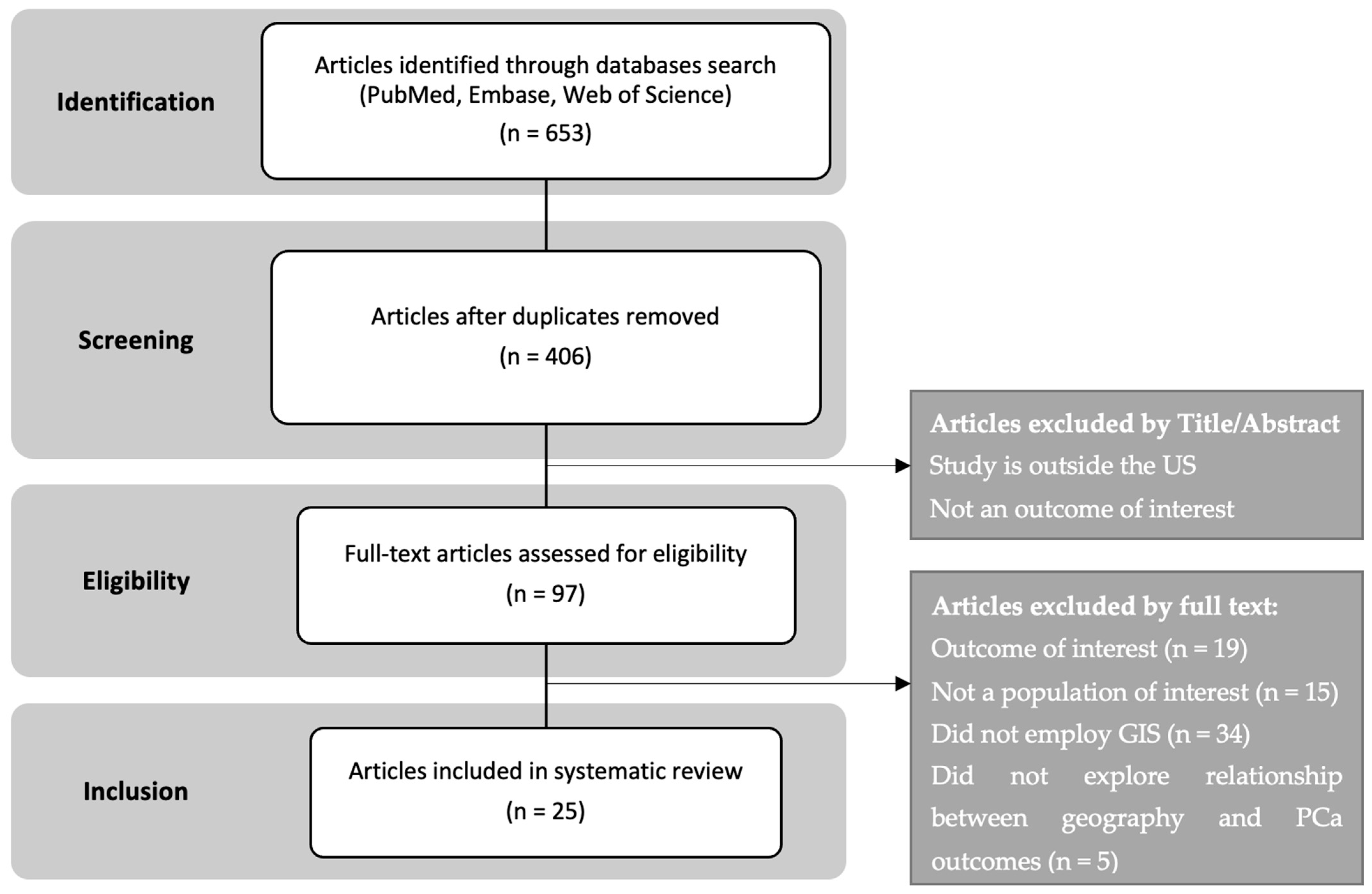
2. Methods
2.1. Search Method
2.2. Article Selection
2.3. Study Management
3. Results
- Higher PCa incidence was frequently associated with better socioeconomic status (SES) at the census-tract level, particularly in non-Hispanic Whites (NHWs) compared to African Americans (AAs).
- Urban residence and higher household income were linked to an increased likelihood of PCa diagnosis, suggesting enhanced healthcare access in these areas.
- The spatial variations in PCa incidence were influenced by factors such as income and education and comorbidities like diabetes and obesity.
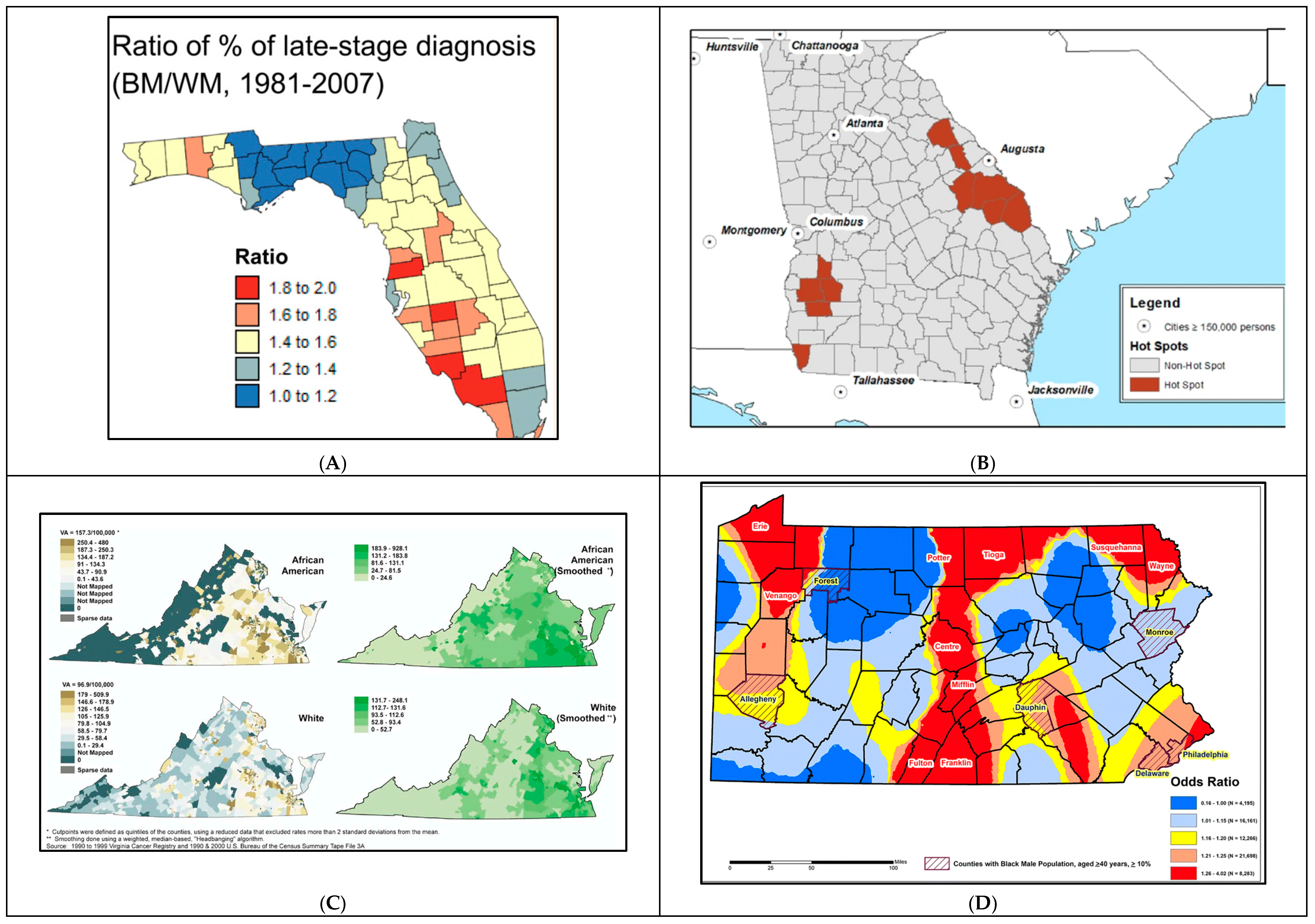
- Disparities in late-stage diagnosis were associated with lower SES, particularly in counties with lower income and education levels.
- Missing stage and grade information served as proxies for worse outcomes and were more common in areas with higher SES, suggesting discrepancies in data collection and reporting.
- Temporal analysis revealed that disparities in late-stage PCa diagnosis have declined over time, influenced by changes in PSA screening recommendations.
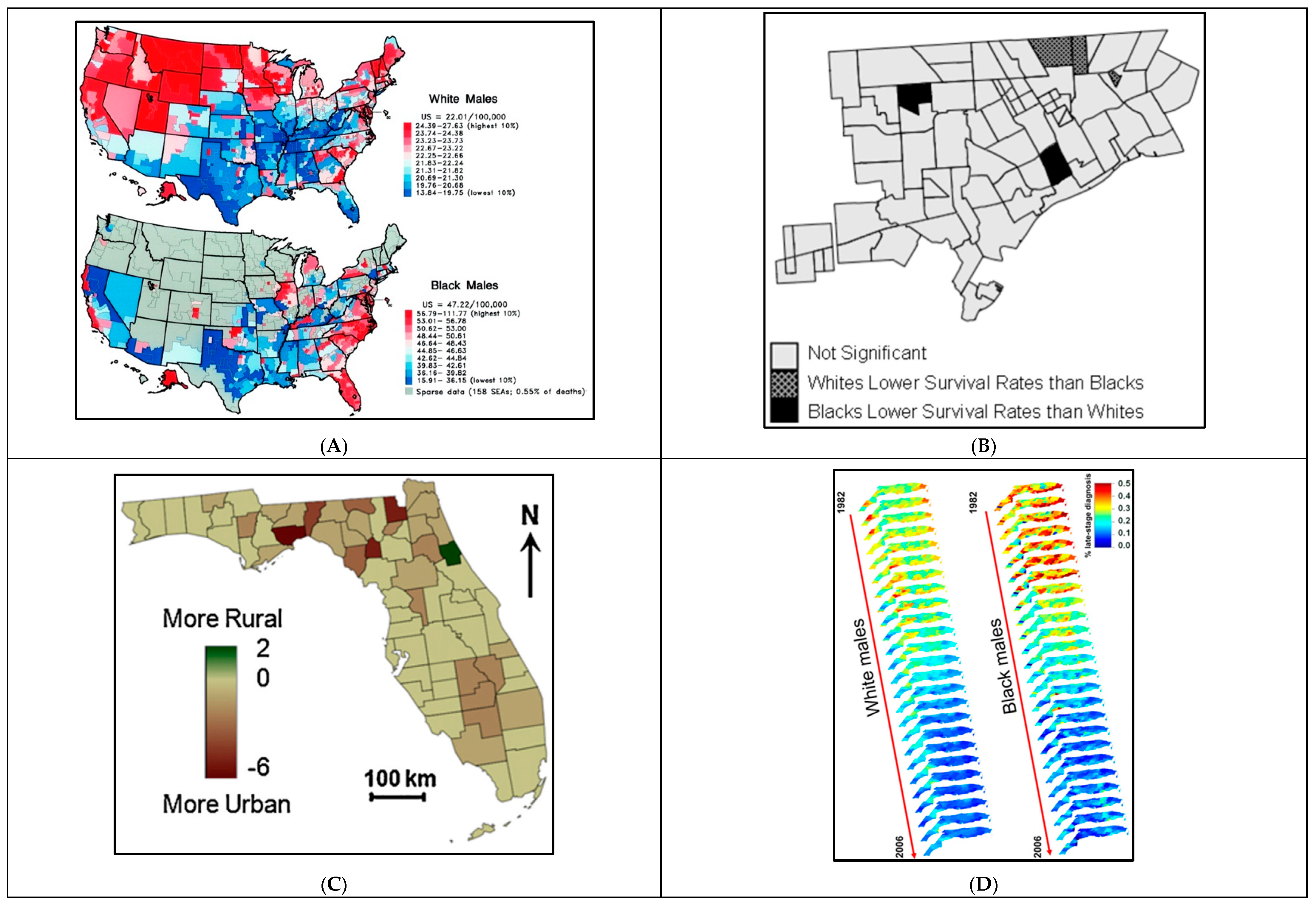
- Geographical clusters of higher mortality rates were identified, with some areas showing significant disparities between racial groups.
- Survival rates varied significantly based on place of residence, with SES factors partially explaining these differences.
- Mapping studies highlighted that rural areas and those with higher poverty rates exhibited poorer PCa survival outcomes.
- Disparities in PCa management were examined in two studies, with GIS mapping showing that treatment modalities were concentrated in urban areas.
- Travel distance impacted the likelihood of receiving certain treatments, with longer distances associated with a decreased probability of intervention.
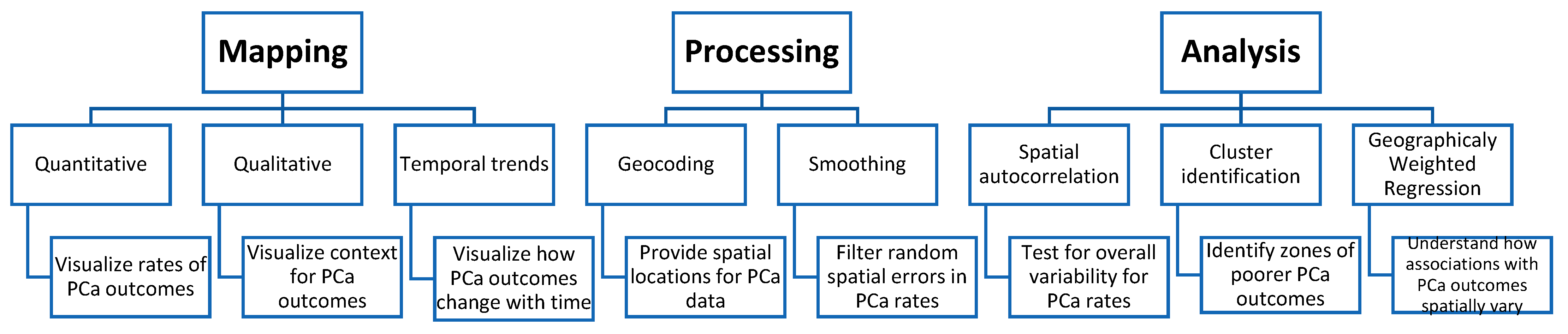
- GIS techniques were predominantly employed for mapping and visualization, translating PCa data into geographical polygons to provide a cartographic representation of PCa rates and zones of disparity.
- Mapping studies commonly used various geographical scales such as counties, census tracts, zip codes, neighborhoods, and census block groups.
- Visual mapping helped identify areas with higher PCa incidence and poorer outcomes, aiding in targeting further analysis and public health interventions.
- Geocoding and smoothing were key GIS processing techniques used to prepare PCa data for analysis.
- Geocoding converted addresses into geographical coordinates, facilitating the visualization of individual-level data at various scales.
- Smoothing techniques like binomial kriging and spatial empirical Bayesian smoothing were used to reduce noise and provide clearer spatial patterns in the data.
- Spatial analysis methods identified geographic associations with PCa outcomes, utilizing techniques like global spatial autocorrelation and cluster identification.
- Global spatial autocorrelation assessed the overall geographical variability and clustering in PCa data.
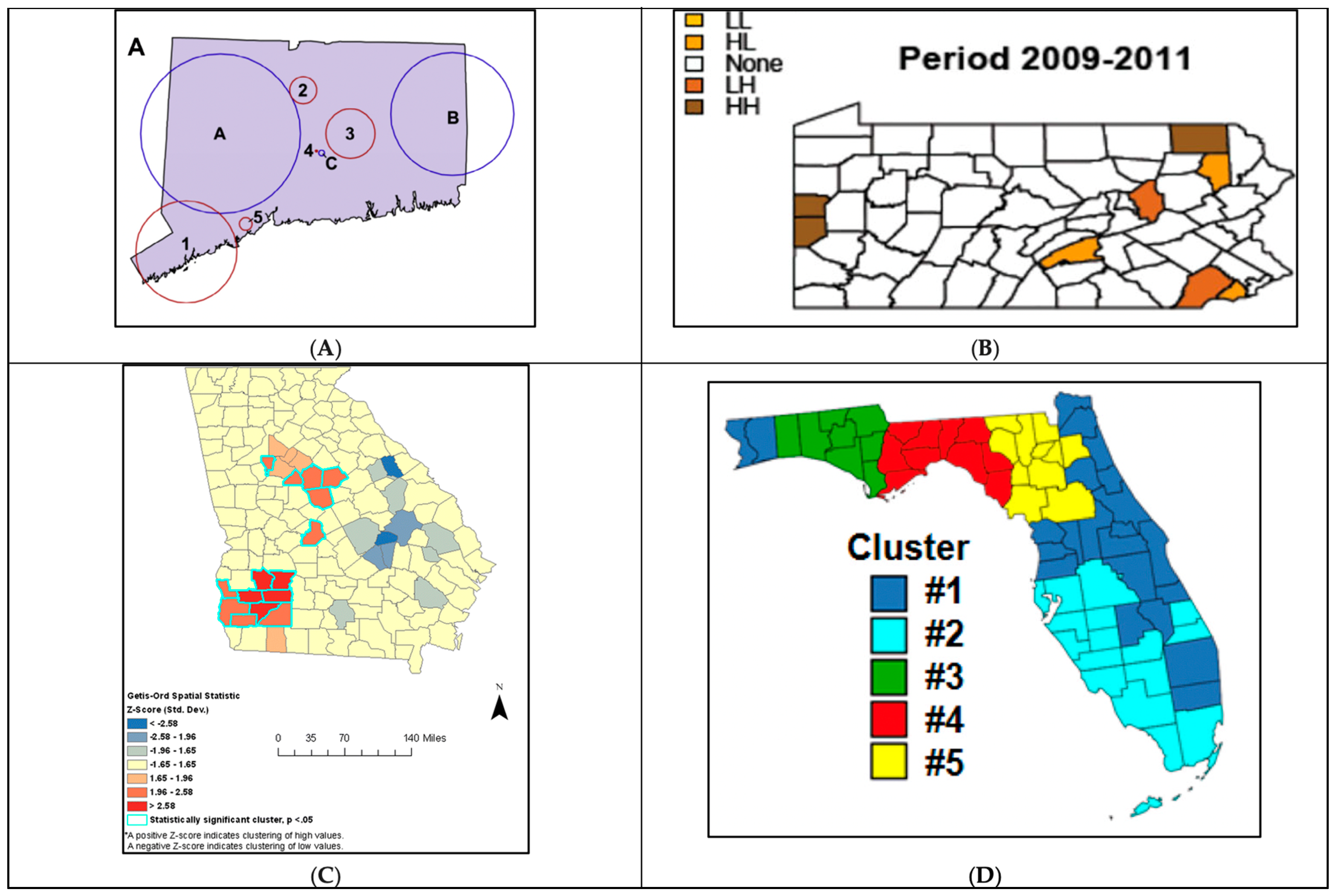
- Cluster identification techniques such as the Spatial Scan Statistic, Getis-Ord-Gi, and local Moran’s I highlighted areas with significant PCa disparities, aiding in prioritizing public health interventions.
- A geographically weighted regression model was employed to examine spatially varying associations between predictors and PCa outcomes, highlighting areas where risk factors had a stronger influence.
4. Summary of PCa Disparities Findings in GIS Studies
4.1. GIS Studies That Examined Disparities in PCa Incidence
4.2. GIS Studies That Examined Disparities in PCa Grade and Stage at Diagnosis
4.3. GIS Studies That Examined Disparities in PCa Mortality and Survival
4.4. GIS Studies That Examined Disparities in PCa Management
5. Application of GIS in PCa Disparities Research
6. Application of GIS in PCa Disparities Research: Mapping
6.1. Mapping a Snapshot in Time: Qualitative and Quantitative Data
6.2. Mapping Trends Overtime
7. Application of GIS in PCa Disparities Research: Processing
7.1. GIS Processing: Geocoding
7.2. GIS Processing: Smoothing
8. Application of GIS in PCa Disparities Research: Spatial Analysis
8.1. GIS Analysis: Identification of Spatial Autocorrelation
8.2. GIS Analysis: Cluster Identification
8.3. GIS Analysis: Geographically Weighted Regression (GWR)
9. Discussion
9.1. Main Themes and Findings
9.2. Specific GIS Applications in PCa Management
9.3. Multilevel Analyses in GIS Research
9.4. Limitations and Recommendations for GIS Mapping, Processing, and Analysis in PCa Disparities Research
9.5. Future Recommendations for GIS Application in PCa Research and Policy Implications
- Expanding the scope to include treatment and management outcomes is crucial. Utilizing comprehensive databases like SEER-Medicare and SPARCS for procedure-level information will provide valuable insights into healthcare access and utilization, leading to a more holistic understanding of PCa disparities.
- Incorporating both spatial and temporal dimensions in GIS research will allow for a more comprehensive assessment of the cancer burden. This can be achieved through preliminary stratification, joinpoint analysis, or detailed discussions that account for ongoing medical advancements and changes in screening recommendations.
- Ensuring racial inclusivity in study populations is also vital. Future research should extend beyond African Americans (AAs) and non-Hispanic Whites (NHWs) to include other minority groups such as non-Hispanic Asian/Pacific Islanders (NHAPI). This will provide a broader understanding of racial disparities in PCa outcomes.
- Combining multiple geospatial approaches for robust cluster detection and sensitivity analysis will enhance the reliability and validity of research findings. Employing techniques like Spatial Scan Statistic (SSS), Local Indicator of Spatial Autocorrelation (LISA), spatial oblique decision trees (SpODT), and hierarchical Bayesian spatial modeling (HBSM) will offer a comprehensive view of spatial patterns and their underlying causes.
- Addressing geocoding quality and the Modifiable Areal Unit Problem (MAUP) is essential. Researchers should adhere to standardized geocoding principles and report geocoding success rates. Conducting sensitivity analyses across different geographical scales and using original point data when possible will mitigate issues related to MAUP and enhance the robustness of findings.
- Leveraging GIS to identify high-risk regions: GIS mapping has identified specific regions, such as the Mississippi Delta, Appalachia, and parts of the Deep South, with significantly higher PCa mortality and lower survival rates. Continuing to utilize GIS in this aspect has the potential to outline the most deprived areas, in the highest needs of public health interventions.
- Implementing GIS mapping of PCa outcomes for a roadmap toward enhanced healthcare access. Geographical locations of poor PCa outcomes can help deploy mobile screening units and expand telemedicine services to ensure early detection and continuous care for PCa patients in rural and underserved urban areas.
- Addressing Socioeconomic Barriers and implementing financial assistance programs to subsidize the cost of PCa screening, diagnosis, and treatment for low-income populations.
- Launching targeted community-based education and awareness campaigns to inform the public about PCa risks, the importance of early detection, and available healthcare resources.
- Improving Data Collection and Reporting by adopting standardized geocoding methods to enhance the accuracy and comparability of spatial data and facilitate better identification of disparities. It is thus important to foster data sharing between cancer registries, healthcare providers, and public health agencies to support comprehensive analyses and tailored interventions.
- Using GIS mapping to improve travel delays associated with public transportation, especially for minority groups, can enhance PCa care [86]. GIS can identify areas with significant delays, helping optimize transit routes and healthcare facility locations to ensure better access to care.
9.6. Study Strengths and Limitations
10. Conclusions
Funding
Data Availability Statement
Acknowledgments
Conflicts of Interest
Appendix A. Research Strategy
| Research Question | ||
| State Question: What are the different geospatial approaches for quantifying health disparities in prostate cancer outcomes? Specific Inclusions/Exclusions: Inclusion: Studies that examine disparities in PCa using geographical elements as independent variables Exclusion: Studies conducted outside the US, studies that did not assess for a direct relationship between a geographical component and PCa disparities were excluded. | Select Core Databases: PubMed Embase Web of Science | Limits: English only Years: Up to 2022 Age Groups: Adults 18 years and older |
| Concept: Health Disparities | Concept: Geospatial Analysis | Concept: Prostate Cancer | |
| Thesaurus Terms/Subheadings | “Socioeconomic Factors”[Mesh] OR “Health Status Disparities”[Mesh] OR “Healthcare Disparities”[Mesh] OR “Health Services Accessibility”[Mesh] OR “Vulnerable Populations”[Mesh] OR | “Geospatial analysis”[MeSH Terms] OR “geographic [MeSH]) OR (geographical[MeSH]) OR (spatial[MeSH]) | “Prostatic Neoplasms”[Mesh] OR |
| Textwords | socioeconomic* OR disparit* OR vulnerable OR “healthcare access” OR “healthcare accessibility” OR “health service accessibility” OR “health services accessibility” | Geograph* OR Spatial OR Geospatial OR GIS OR Place of Residence OR Mapping | “prostate cancer” OR “prostate cancers” OR “cancer of the prostate” OR “prostatic neoplasms” OR “prostate neoplasms” |
| Search Number | Query | Search Details | Results |
| 4 | (((“Prostatic Neoplasms”[Mesh] OR “prostate cancer” OR “prostate cancers” OR “cancer of the prostate” OR “prostatic neoplasms” OR “prostate neoplasms”)) AND ((“Socioeconomic Factors”[Mesh] OR “Health Status Disparities”[Mesh] OR “Healthcare Disparities”[Mesh] OR “Health Services Accessibility”[Mesh] OR “Vulnerable Populations”[Mesh] OR socioeconomic* OR disparit* OR vulnerable OR “healthcare access” OR “healthcare accessibility” OR “health service accessibility” OR “health services accessibility”)))) AND (“Geography”[Mesh] OR “Geography, Medical”[Mesh] OR geograph* OR spatial OR geospatial* OR geospatial analysis OR GIS OR Mapping OR “Place of Residence”) Filters: English | (“Prostatic Neoplasms”[MeSH Terms] OR “prostate cancer”[All Fields] OR “prostate cancers”[All Fields] OR “cancer of the prostate”[All Fields] OR “Prostatic Neoplasms”[All Fields] OR “prostate neoplasms”[All Fields]) AND (“Socioeconomic Factors”[MeSH Terms] OR “Health Status Disparities”[MeSH Terms] OR “Healthcare Disparities”[MeSH Terms] OR “Health Services Accessibility”[MeSH Terms] OR “Vulnerable Populations”[MeSH Terms] OR “socioeconomic*”[All Fields] OR “disparit*”[All Fields] OR (“vulnerabilities”[All Fields] OR “vulnerability”[All Fields] OR “vulnerable”[All Fields] OR “vulnerables”[All Fields]) OR “healthcare access”[All Fields] OR “healthcare accessibility”[All Fields] OR “health service accessibility”[All Fields] OR “Health Services Accessibility”[All Fields]) AND (“Geography”[MeSH Terms] OR “geography, medical”[MeSH Terms] OR “geograph*”[All Fields] OR (“spatial”[All Fields] OR “spatialization”[All Fields] OR “spatializations”[All Fields] OR “spatialized”[All Fields] OR “spatially”[All Fields]) OR “geospatial*”[All Fields] OR ((“geospatial”[All Fields] OR “geospatially”[All Fields]) AND (“analysis”[MeSH Subheading] OR “analysis”[All Fields])) OR (“proc acm sigspatial int conf adv inf”[Journal] OR “gis”[All Fields]) OR (“mapped”[All Fields] OR “mapping”[All Fields] OR “mappings”[All Fields]) OR “Place of Residence”[All Fields]) | 320 |
| 3 | “Geography”[Mesh] OR “Geography, Medical”[Mesh] OR geograph* OR spatial OR geospatial* OR geospatial analysis OR GIS OR Mapping OR “Place of Residence” | “Geography”[MeSH Terms] OR “geography, medical”[MeSH Terms] OR “geograph*”[All Fields] OR (“spatial”[All Fields] OR “spatialization”[All Fields] OR “spatializations”[All Fields] OR “spatialized”[All Fields] OR “spatially”[All Fields]) OR “geospatial*”[All Fields] OR ((“geospatial”[All Fields] OR “geospatially”[All Fields]) AND (“analysis”[MeSH Subheading] OR “analysis”[All Fields])) OR (“proc acm sigspatial int conf adv inf”[Journal] OR “gis”[All Fields]) OR (“mapped”[All Fields] OR “mapping”[All Fields] OR “mappings”[All Fields]) OR “Place of Residence”[All Fields] | 1,116,497 |
| 2 | (“Socioeconomic Factors”[Mesh] OR “Health Status Disparities”[Mesh] OR “Healthcare Disparities”[Mesh] OR “Health Services Accessibility”[Mesh] OR “Vulnerable Populations”[Mesh] OR socioeconomic* OR disparit* OR vulnerable OR “healthcare access” OR “healthcare accessibility” OR “health service accessibility” OR “health services accessibility”)) | “Socioeconomic Factors”[MeSH Terms] OR “Health Status Disparities”[MeSH Terms] OR “Healthcare Disparities”[MeSH Terms] OR “Health Services Accessibility”[MeSH Terms] OR “Vulnerable Populations”[MeSH Terms] OR “socioeconomic*”[All Fields] OR “disparit*”[All Fields] OR “vulnerabilities”[All Fields] OR “vulnerability”[All Fields] OR “vulnerable”[All Fields] OR “vulnerables”[All Fields] OR “healthcare access”[All Fields] OR “healthcare accessibility”[All Fields] OR “health service accessibility”[All Fields] OR “Health Services Accessibility”[All Fields] | 950,029 |
| 1 | (“Prostatic Neoplasms”[Mesh] OR “prostate cancer” OR “prostate cancers” OR “cancer of the prostate” OR “prostatic neoplasms” OR “prostate neoplasms”) | “Prostatic Neoplasms”[MeSH Terms] OR “prostate cancer”[All Fields] OR “prostate cancers”[All Fields] OR “cancer of the prostate”[All Fields] OR “Prostatic Neoplasms”[All Fields] OR “prostate neoplasms”[All Fields] | 184,831 |
| No. | Query | Results |
| #4 | #1 AND #2 AND #3 | 317 |
| #3 | (‘geography’ OR ‘geography, medical’ OR geograph* OR spatial OR geospatial* OR geospatial) AND analysis OR gis OR mapping OR ‘place of residence’ | 682,890 |
| #2 | ‘socioeconomic factors’ OR ‘health status disparities’ OR ‘healthcare disparities’ OR ‘vulnerable populations’ OR socioeconomic* OR disparit* OR vulnerable OR ‘healthcare access’ OR ‘healthcare accessibility’ OR ‘health service accessibility’ OR ‘health services accessibility’ | 583,093 |
| #1 | ‘prostatic neoplasms’/exp OR ‘prostatic neoplasms’ | 291,595 |
| Query | Results |
| (‘prostatic neoplasms’ OR ‘prostatic neoplasms’) AND (‘socioeconomic factors’ OR ‘health status disparities’ OR ‘healthcare disparities’ OR ‘vulnerable populations’ OR socioeconomic* OR disparit* OR vulnerable OR ‘healthcare access’ OR ‘healthcare accessibility’ OR ‘health service accessibility’ OR ‘health services accessibility’) AND ((‘geography’ OR ‘geography, medical’ OR geograph* OR spatial OR geospatial* OR geospatial) AND analysis OR gis OR mapping OR ‘place of residence’) | 16 |
| ((‘geography’ OR ‘geography, medical’ OR geograph* OR spatial OR geospatial* OR geospatial) AND analysis OR gis OR mapping OR ‘place of residence’) | 3,173,703 |
| (‘socioeconomic factors’ OR ‘health status disparities’ OR ‘healthcare disparities’ OR ‘vulnerable populations’ OR socioeconomic* OR disparit* OR vulnerable OR ‘healthcare access’ OR ‘healthcare accessibility’ OR ‘health service accessibility’ OR ‘health services accessibility’) | 629,895 |
| (‘prostatic neoplasms’ OR ‘prostatic neoplasms’) | 8363 |
References
- Zavala, V.A.; Bracci, P.M.; Carethers, J.M.; Carvajal-Carmona, L.; Coggins, N.B.; Cruz-Correa, M.R.; Davis, M.; de Smith, A.J.; Dutil, J.; Figueiredo, J.C.; et al. Cancer health disparities in racial/ethnic minorities in the United States. Br. J. Cancer 2021, 124, 315–332. [Google Scholar] [CrossRef] [PubMed] [PubMed Central]
- Rawla, P. Epidemiology of Prostate Cancer. World J. Oncol. 2019, 10, 63–89. [Google Scholar] [CrossRef] [PubMed] [PubMed Central]
- Coughlin, S.S. A review of social determinants of prostate cancer risk, stage, and survival. Prostate Int. 2020, 8, 49–54. [Google Scholar] [CrossRef] [PubMed] [PubMed Central]
- Siegel, R.L.; Miller, K.D.; Jemal, A. Cancer statistics, 2020. CA Cancer J. Clin. 2020, 70, 7–30. [Google Scholar] [CrossRef] [PubMed]
- DeSantis, C.E.; Miller, K.D.; Goding Sauer, A.; Jemal, A.; Siegel, R.L. Cancer statistics for African Americans, 2019. CA Cancer J. Clin. 2019, 69, 211–233. [Google Scholar] [CrossRef] [PubMed]
- Chornokur, G.; Dalton, K.; Borysova, M.E.; Kumar, N.B. Disparities at presentation, diagnosis, treatment, and survival in African American men, affected by prostate cancer. Prostate 2011, 71, 985–997. [Google Scholar] [CrossRef] [PubMed] [PubMed Central]
- Dess, R.T.; Hartman, H.E.; Mahal, B.A.; Soni, P.D.; Jackson, W.C.; Cooperberg, M.R.; Amling, C.L.; Aronson, W.J.; Kane, C.J.; Terris, M.K.; et al. Association of Black Race with Prostate Cancer-Specific and Other-Cause Mortality. JAMA Oncol. 2019, 5, 975–983. [Google Scholar] [CrossRef] [PubMed] [PubMed Central]
- Tyson, M.D., 2nd; Castle, E.P. Racial disparities in survival for patients with clinically localized prostate cancer adjusted for treatment effects. Mayo Clin. Proc. 2014, 89, 300–307. [Google Scholar] [CrossRef] [PubMed]
- Pinheiro, P.S.; Sherman, R.L.; Trapido, E.J.; Fleming, L.E.; Huang, Y.; Gomez-Marin, O.; Lee, D. Cancer incidence in first generation U.S. Hispanics: Cubans, Mexicans, Puerto Ricans, and new Latinos. Cancer Epidemiol. Biomark. Prev. 2009, 18, 2162–2169. [Google Scholar] [CrossRef] [PubMed]
- Ho, G.Y.; Figueroa-Valles, N.R.; De La Torre-Feliciano, T.; Tucker, K.L.; Tortolero-Luna, G.; Rivera, W.T.; Jiménez-Velázquez, I.Z.; Ortiz-Martínez, A.P.; Rohan, T.E. Cancer disparities between mainland and island Puerto Ricans. Rev. Panam. Salud Publica 2009, 25, 394–400. [Google Scholar] [CrossRef] [PubMed]
- Dasgupta, P.; Baade, P.D.; Aitken, J.F.; Ralph, N.; Chambers, S.K.; Dunn, J. Geographical Variations in Prostate Cancer Outcomes: A Systematic Review of International Evidence. Front. Oncol. 2019, 9, 238. [Google Scholar] [CrossRef] [PubMed] [PubMed Central]
- Baade, P.D.; Yu, X.Q.; Smith, D.P.; Dunn, J.; Chambers, S.K. Geographic disparities in prostate cancer outcomes—Review of international patterns. Asian Pac. J. Cancer Prev. 2015, 16, 1259–1275. [Google Scholar] [CrossRef] [PubMed]
- Obertova, Z.; Brown, C.; Holmes, M.; Lawrenson, R. Prostate cancer incidence and mortality in rural men—A systematic review of the literature. Rural. Remote Health 2012, 12, 2039. [Google Scholar] [CrossRef] [PubMed]
- Afshar, N.; English, D.R.; Milne, R.L. Rural-urban residence and cancer survival in high-income countries: A systematic review. Cancer 2019, 125, 2172–2184. [Google Scholar] [CrossRef] [PubMed]
- Gilbert, S.M.; Pow-Sang, J.M.; Xiao, H. Geographical Factors Associated with Health Disparities in Prostate Cancer. Cancer Control 2016, 23, 401–408. [Google Scholar] [CrossRef] [PubMed]
- Research NCIGPfC. Health Disparities Information. Available online: https://giscancergov/research/health_disparitieshrml (accessed on 15 November 2022).
- Cobb, C.D. Geospatial Analysis: A New Window Into Educational Equity, Access, and Opportunity. Rev. Res. Educ. 2020, 44, 97–129. [Google Scholar] [CrossRef]
- Adebola, T.M.; Fennell, H.W.W.; Druitt, M.D.; Bonin, C.A.; Jenifer, V.A.; van Wijnen, A.J.; Lewallen, E.A. Population-Level Patterns of Prostate Cancer Occurrence: Disparities in Virginia. Curr. Mol. Biol. Rep. 2022, 8, 1–8. [Google Scholar] [CrossRef] [PubMed] [PubMed Central]
- Freeman, V.L.; Ricardo, A.C.; Campbell, R.T.; Barrett, R.E.; Warnecke, R.B. Association of census tract-level socioeconomic status with disparities in prostate cancer-specific survival. Cancer Epidemiol. Biomark. Prev. 2011, 20, 2150–2159. [Google Scholar] [CrossRef] [PubMed] [PubMed Central]
- Washington, C.; Deville, C., Jr. Health disparities and inequities in the utilization of diagnostic imaging for prostate cancer. Abdom. Radiol. 2020, 45, 4090–4096. [Google Scholar] [CrossRef] [PubMed]
- Ajayi, A.; Hwang, W.T.; Vapiwala, N.; Rosen, M.; Chapman, C.H.; Both, S.; Shah, M.; Wang, X.; Agawu, A.; Gabriel, P.; et al. Disparities in staging prostate magnetic resonance imaging utilization for nonmetastatic prostate cancer patients undergoing definitive radiation therapy. Adv. Radiat. Oncol. 2016, 1, 325–332. [Google Scholar] [CrossRef] [PubMed] [PubMed Central]
- El Khoury, C.J.; Ros, P.R. A Systematic Review for Health Disparities and Inequities in Multiparametric Magnetic Resonance Imaging for Prostate Cancer Diagnosis. Acad. Radiol. 2021, 28, 953–962. [Google Scholar] [CrossRef] [PubMed]
- Orom, H.; Biddle, C.; Underwood, W., 3rd; Homish, G.G.; Olsson, C.A. Racial or Ethnic and Socioeconomic Disparities in Prostate Cancer Survivors’ Prostate-specific Quality of Life. Urology 2018, 112, 132–137. [Google Scholar] [CrossRef] [PubMed] [PubMed Central]
- Beale, L.; Abellan, J.J.; Hodgson, S.; Jarup, L. Methodologic issues and approaches to spatial epidemiology. Environ. Health Perspect. 2008, 116, 1105–1110. [Google Scholar] [CrossRef] [PubMed] [PubMed Central]
- Seidman, C.S. An introduction to prostate cancer and geographic information systems. Am. J. Prev. Med. 2006, 30 (Suppl. S2), S1–S2. [Google Scholar] [CrossRef] [PubMed]
- Mark, D.M. Geographic information science: Defining the field. In Foundations of Geographic Information Science; Duckham, M., Goodchild, M.F., Worboys, M.F., Eds.; Taylor & Francis: New York, NY, USA, 2003; pp. 3–18. [Google Scholar]
- University Consortium for Geographic Information Science (UCGIS). UCGIS Bylaws, 2016 Version; 2016 Version; UCGIS: Washington, DC, USA, 2016; Available online: http://wwwucgisorg/assets/docs/ucgis_bylaws_march2016pdf (accessed on 15 December 2022).
- Sahar, L.; Foster, S.L.; Sherman, R.L.; Henry, K.A.; Goldberg, D.W.; Stinchcomb, D.G.; Bauer, J.E. GIScience and cancer: State of the art and trends for cancer surveillance and epidemiology. Cancer 2019, 125, 2544–2560. [Google Scholar] [CrossRef] [PubMed] [PubMed Central]
- Elliott, P.; Wartenberg, D. Spatial epidemiology: Current approaches and future challenges. Environ. Health Perspect. 2004, 112, 998–1006. [Google Scholar] [CrossRef] [PubMed] [PubMed Central]
- Lyseen, A.K.; Nohr, C.; Sorensen, E.M.; Gudes, O.; Geraghty, E.M.; Shaw, N.T.; Bivona-Tellez, C.; Lyseen, A.K.; The IMIA Health GIS Working Group. A Review and Framework for Categorizing Current Research and Development in Health Related Geographical Information Systems (GIS) Studies. Yearb. Med. Inf. 2014, 9, 110–124. [Google Scholar] [CrossRef] [PubMed] [PubMed Central]
- DeRouen, M.C.; Schupp, C.W.; Koo, J.; Yang, J.; Hertz, A.; Shariff-Marco, S.; Cockburn, M.; Nelson, D.O.; Ingles, S.A.; John, E.M.; et al. Impact of individual and neighborhood factors on disparities in prostate cancer survival. Cancer Epidemiol. 2018, 53, 1–11. [Google Scholar] [CrossRef] [PubMed] [PubMed Central]
- DeRouen, M.C.; Schupp, C.W.; Yang, J.; Koo, J.; Hertz, A.; Shariff-Marco, S.; Cockburn, M.; Nelson, D.O.; Ingles, S.A.; Cheng, I.; et al. Impact of individual and neighborhood factors on socioeconomic disparities in localized and advanced prostate cancer risk. Cancer Causes Control 2018, 29, 951–966. [Google Scholar] [CrossRef] [PubMed] [PubMed Central]
- Higgins, J.P.; Altman, D.G.; Gotzsche, P.C.; Juni, P.; Moher, D.; Oxman, A.D.; Savović, J.; Schulz, K.F.; Weeks, L.; Sterne, J.A.C.; et al. The Cochrane Collaboration’s tool for assessing risk of bias in randomised trials. BMJ 2011, 343, d5928. [Google Scholar] [CrossRef] [PubMed] [PubMed Central]
- Liberati, A.; Altman, D.G.; Tetzlaff, J.; Mulrow, C.; Gotzsche, P.C.; Ioannidis, J.P.; Clarke, M.; Devereaux, P.J.; Kleijnen, J.; Moher, D. The PRISMA statement for reporting systematic reviews and meta-analyses of studies that evaluate healthcare interventions: Explanation and elaboration. BMJ 2009, 339, b2700. [Google Scholar] [CrossRef] [PubMed] [PubMed Central]
- PubMED. Available online: https://pubmedncbinlmnihgov (accessed on 15 December 2021).
- EMBASE. Available online: https://wwwembasecom/landing?status=grey (accessed on 15 December 2021).
- Web of Science-Clarivate. Available online: https://wwwwebofsciencecom/wos/woscc/basic-search (accessed on 15 December 2021).
- Jemal, A.; Kulldorff, M.; Devesa, S.S.; Hayes, R.B.; Fraumeni, J.F., Jr. A geographic analysis of prostate cancer mortality in the United States, 1970–1989. Int. J. Cancer 2002, 101, 168–174. [Google Scholar] [CrossRef] [PubMed]
- Klassen, A.C.; Kulldorff, M.; Curriero, F. Geographical clustering of prostate cancer grade and stage at diagnosis, before and after adjustment for risk factors. Int. J. Health Geogr. 2005, 4, 1. [Google Scholar] [CrossRef] [PubMed] [PubMed Central]
- DeChello, L.M.; Gregorio, D.I.; Samociuk, H. Race-specific geography of prostate cancer incidence. Int. J. Health Geogr. 2006, 5, 59. [Google Scholar] [CrossRef] [PubMed] [PubMed Central]
- Oliver, M.N.; Smith, E.; Siadaty, M.; Hauck, F.R.; Pickle, L.W. Spatial analysis of prostate cancer incidence and race in Virginia, 1990–1999. Am. J. Prev. Med. 2006, 30 (Suppl. S2), S67–S76. [Google Scholar] [CrossRef] [PubMed]
- Gregorio, D.I.; Huang, L.; DeChello, L.M.; Samociuk, H.; Kulldorff, M. Place of residence effect on likelihood of surviving prostate cancer. Ann. Epidemiol. 2007, 17, 520–524. [Google Scholar] [CrossRef] [PubMed]
- Xiao, H.; Gwede, C.K.; Kiros, G.; Milla, K. Analysis of prostate cancer incidence using geographic information system and multilevel modeling. J. Natl. Med. Assoc. 2007, 99, 218–225. [Google Scholar] [PubMed] [PubMed Central]
- Hsu, C.E.; Mas, F.S.; Miller, J.A.; Nkhoma, E.T. A spatial-temporal approach to surveillance of prostate cancer disparities in population subgroups. J. Natl. Med. Assoc. 2007, 99, 72–80, 85–87. [Google Scholar] [PubMed] [PubMed Central]
- Hinrichsen, V.L.; Klassen, A.C.; Song, C.; Kulldorff, M. Evaluation of the performance of tests for spatial randomness on prostate cancer data. Int. J. Health Geogr. 2009, 8, 41. [Google Scholar] [CrossRef] [PubMed] [PubMed Central]
- Meliker, J.R.; Goovaerts, P.; Jacquez, G.M.; Avruskin, G.A.; Copeland, G. Breast and prostate cancer survival in Michigan: Can geographic analyses assist in understanding racial disparities? Cancer 2009, 115, 2212–2221. [Google Scholar] [CrossRef] [PubMed] [PubMed Central]
- Hebert, J.R.; Daguise, V.G.; Hurley, D.M.; Wilkerson, R.C.; Mosley, C.M.; Adams, S.A.; Puett, R.; Burch, J.B.; Steck, S.E.; Bolick-Aldrich, S.W. Mapping cancer mortality-to-incidence ratios to illustrate racial and sex disparities in a high-risk population. Cancer 2009, 115, 2539–2552. [Google Scholar] [CrossRef] [PubMed] [PubMed Central]
- Altekruse, S.F.; Huang, L.; Cucinelli, J.E.; McNeel, T.S.; Wells, K.M.; Oliver, M.N. Spatial patterns of localized-stage prostate cancer incidence among white and black men in the southeastern United States, 1999–2001. Cancer Epidemiol. Biomark. Prev. 2010, 19, 1460–1467. [Google Scholar] [CrossRef] [PubMed] [PubMed Central]
- Goovaerts, P.; Xiao, H. Geographical, temporal and racial disparities in late-stage prostate cancer incidence across Florida: A multiscale joinpoint regression analysis. Int. J. Health Geogr. 2011, 10, 63. [Google Scholar] [CrossRef] [PubMed] [PubMed Central]
- Xiao, H.; Tan, F.; Goovaerts, P. Racial and geographic disparities in late-stage prostate cancer diagnosis in Florida. J. Health Care Poor Underserved 2011, 22 (Suppl. S4), 187–199. [Google Scholar] [CrossRef] [PubMed] [PubMed Central]
- Goovaerts, P.; Xiao, H. The impact of place and time on the proportion of late-stage diagnosis: The case of prostate cancer in Florida, 1981–2007. Spat. Spatiotemporal Epidemiol. 2012, 3, 243–253. [Google Scholar] [CrossRef] [PubMed] [PubMed Central]
- Goovaerts, P. Analysis of geographical disparities in temporal trends of health outcomes using space-time joinpoint regression. Int. J. Appl. Earth Obs. Geoinf. 2013, 22, 75–85. [Google Scholar] [CrossRef] [PubMed] [PubMed Central]
- Wagner, S.E.; Bauer, S.E.; Bayakly, A.R.; Vena, J.E. Prostate cancer incidence and tumor severity in Georgia: Descriptive epidemiology, racial disparity, and geographic trends. Cancer Causes Control 2013, 24, 153–166. [Google Scholar] [CrossRef] [PubMed]
- Gregorio, D.I.; Samociuk, H. Prostate cancer incidence in light of the spatial distribution of another screening-detectable cancer. Spat. Spatiotemporal Epidemiol. 2013, 6, 1–6. [Google Scholar] [CrossRef] [PubMed]
- Goovaerts, P.; Xiao, H.; Adunlin, G.; Ali, A.; Tan, F.; Gwede, C.K.; Huang, Y. Geographically-Weighted Regression Analysis of Percentage of Late-Stage Prostate Cancer Diagnosis in Florida. Appl. Geogr. 2015, 62, 191–200. [Google Scholar] [CrossRef] [PubMed] [PubMed Central]
- Wang, M.; Matthews, S.A.; Iskandarani, K.; Li, Y.; Li, Z.; Chinchilli, V.M.; Zhang, L. Spatial-temporal analysis of prostate cancer incidence from the Pennsylvania Cancer Registry, 2000–2011. Geospat. Health 2017, 12, 611. [Google Scholar] [CrossRef] [PubMed] [PubMed Central]
- Wang, M.; Chi, G.; Bodovski, Y.; Holder, S.L.; Lengerich, E.J.; Wasserman, E.; McDonald, A.C. Temporal and spatial trends and determinants of aggressive prostate cancer among Black and White men with prostate cancer. Cancer Causes Control 2020, 31, 63–71. [Google Scholar] [CrossRef] [PubMed]
- Aghdam, N.; Carrasquilla, M.; Wang, E.; Pepin, A.N.; Danner, M.; Ayoob, M.; Yung, T.; Collins, B.T.; Kumar, D.; Suy, S.; et al. Ten-Year Single Institutional Analysis of Geographic and Demographic Characteristics of Patients Treated with Stereotactic Body Radiation Therapy for Localized Prostate Cancer. Front. Oncol. 2020, 10, 616286. [Google Scholar] [CrossRef] [PubMed] [PubMed Central]
- Georgantopoulos, P.; Eberth, J.M.; Cai, B.; Rao, G.; Bennett, C.L.; Emrich, C.T.; Haddock, K.S.; Hébert, J.R. A spatial assessment of prostate cancer mortality-to-incidence ratios among South Carolina veterans: 1999–2015. Ann. Epidemiol. 2021, 59, 24–32. [Google Scholar] [CrossRef] [PubMed]
- Moore, J.X.; Tingen, M.S.; Coughlin, S.S.; O’Meara, C.; Odhiambo, L.; Vernon, M.; Jones, S.; Petcu, R.; Johnson, R.; Islam, K.M.; et al. Understanding geographic and racial/ethnic disparities in mortality from four major cancers in the state of Georgia: A spatial epidemiologic analysis, 1999–2019. Sci. Rep. 2022, 12, 14143. [Google Scholar] [CrossRef] [PubMed] [PubMed Central]
- Aladuwaka, S.; Alagan, R.; Singh, R.; Mishra, M. Health Burdens and SES in Alabama: Using Geographic Information System to Examine Prostate Cancer Health Disparity. Cancers 2022, 14, 4824. [Google Scholar] [CrossRef] [PubMed] [PubMed Central]
- Tang, C.; Lei, X.; Smith, G.L.; Pan, H.Y.; Hoffman, K.E.; Kumar, R.; Chapin, B.F.; Shih, Y.-C.T.; Frank, S.J.; Smith, B.D. Influence of Geography on Prostate Cancer Treatment. Int. J. Radiat. Oncol. Biol. Phys. 2021, 109, 1286–1295. [Google Scholar] [CrossRef] [PubMed] [PubMed Central]
- Moyer, V.A.; US Preventive Services Task Force. Screening for prostate cancer: U.S. Preventive Services Task Force Recommendation Statement. Ann. Intern. Med. 2012, 157, 120–134. [Google Scholar] [CrossRef] [PubMed]
- Maguire, D. ArcGIS: General Purpose GIS Software System. In Encyclopedia of GIS; Shekhar, S., Xiong, H., Eds.; Springer: Boston, MA, USA, 2008. [Google Scholar] [CrossRef]
- Esri, A.P. ArcGIS Online. Available online: https://wwwesricom/en-us/landing-page/product/2019/arcgis-online/overview/ (accessed on 15 December 2021).
- Griffith, D.A. Estimators of Spatial Autocorrelation. Encycl. Social. Meas. 2005, 3, 581. [Google Scholar]
- Tobler, W. A computer movie simulating urban growth in the Detroit Region. Econ. Geogr. 1970, 46, 234–240. [Google Scholar] [CrossRef]
- Kulldorff, M.; Nagarwalla, N. Spatial disease clusters: Detection and inference. Stat. Med. 1995, 14, 799–810. [Google Scholar] [CrossRef] [PubMed]
- Arthur Getis, J.K.O. The Analysis of Spatial Association by Use of Distance Statistics. Geogr. Anal. 1992, 24, 189–206. [Google Scholar] [CrossRef]
- Understanding Prostate Cancer Disparities. Available online: https://wwwccsnwiorg/prostatecancerdisparitieshtml (accessed on 15 December 2021).
- Cackowski, F.C.; Mahal, B.; Heath, E.I.; Carthon, B. Evolution of Disparities in Prostate Cancer Treatment: Is This a New Normal? Am. Soc. Clin. Oncol. Educ. Book. 2021, 41, e203–e214. [Google Scholar] [CrossRef] [PubMed]
- SEER-Medicare Linked Data Resource. Available online: https://healthcaredeliverycancergov/seermedicare/ (accessed on 15 December 2021).
- Statewide Planning and Research Cooperative System (SPARCS). Available online: https://wwwhealthnygov/statistics/sparcs/ (accessed on 15 December 2021).
- Arega, M.A.; Yang, D.D.; Royce, T.J.; Mahal, B.A.; Dee, E.C.; Butler, S.S.; Sha, S.; Mouw, K.W.; Nguyen, P.L.; Muralidhar, V. Association between Travel Distance and Use of Postoperative Radiation Therapy among Men with Organ-Confined Prostate Cancer: Does Geography Influence Treatment Decisions? Pract. Radiat. Oncol. 2021, 11, e426–e433. [Google Scholar] [CrossRef] [PubMed]
- Muralidhar, V.; Rose, B.S.; Chen, Y.W.; Nezolosky, M.D.; Nguyen, P.L. Association between Travel Distance and Choice of Treatment for Prostate Cancer: Does Geography Reduce Patient Choice? Int. J. Radiat. Oncol. Biol. Phys. 2016, 96, 313–317. [Google Scholar] [CrossRef] [PubMed]
- Holmes, J.A.; Carpenter, W.R.; Wu, Y.; Hendrix, L.H.; Peacock, S.; Massing, M.; Schenck, A.P.; Meyer, A.-M.; Diao, K.; Wheeler, S.B.; et al. Impact of distance to a urologist on early diagnosis of prostate cancer among black and white patients. J. Urol. 2012, 187, 883–888. [Google Scholar] [CrossRef] [PubMed]
- Dobbs, R.W.; Malhotra, N.R.; Caldwell, B.M.; Rojas, R.; Moreira, D.M.; Abern, M.R. Determinants of Clinic Absenteeism: A Novel Method of Examining Distance from Clinic and Transportation. J. Community Health 2018, 43, 19–26. [Google Scholar] [CrossRef] [PubMed]
- Teshale, A.B.; Amare, T. Exploring spatial variations and the individual and contextual factors of uptake of measles-containing second dose vaccine among children aged 24 to 35 months in Ethiopia. PLoS ONE 2023, 18, e0280083. [Google Scholar] [CrossRef] [PubMed] [PubMed Central]
- Saha, A.; Hayen, A.; Ali, M.; Rosewell, A.; MacIntyre, C.R.; Clemens, J.D.; Qadri, F. Socioeconomic drivers of vaccine uptake: An analysis of the data of a geographically defined cluster randomized cholera vaccine trial in Bangladesh. Vaccine 2018, 36, 4742–4749. [Google Scholar] [CrossRef] [PubMed] [PubMed Central]
- Zahnd, W.E.; McLafferty, S.L.; Sherman, R.L.; Klonoff-Cohen, H.; Farner, S.; Rosenblatt, K.A. Spatial Accessibility to Mammography Services in the Lower Mississippi Delta Region States. J. Rural. Health 2019, 35, 550–559. [Google Scholar] [CrossRef] [PubMed]
- Grande, D.; Asch, D.A.; Wan, F.; Bradbury, A.R.; Jagsi, R.; Mitra, N. Are Patients with Cancer Less Willing to Share Their Health Information? Privacy, Sensitivity, and Social Purpose. J. Oncol. Pract. 2015, 11, 378–383. [Google Scholar] [CrossRef] [PubMed] [PubMed Central]
- Luo, L.; McLafferty, S.; Wang, F. Analyzing spatial aggregation error in statistical models of late-stage cancer risk: A Monte Carlo simulation approach. Int. J. Health Geogr. 2010, 9, 51. [Google Scholar] [CrossRef] [PubMed] [PubMed Central]
- Goldberg, D.W.; Ballard, M.; Boyd, J.H.; Mullan, N.; Garfield, C.; Rosman, D.; Ferrante, A.M.; Semmens, J.B. An evaluation framework for comparing geocoding systems. Int. J. Health Geogr. 2013, 12, 50. [Google Scholar] [CrossRef] [PubMed] [PubMed Central]
- Oliver, M.N.; Matthews, K.A.; Siadaty, M.; Hauck, F.R.; Pickle, L.W. Geographic bias related to geocoding in epidemiologic studies. Int. J. Health Geogr. 2005, 4, 29. [Google Scholar] [CrossRef] [PubMed] [PubMed Central]
- Geary, R.C. The Contiguity Ratio and Statistical Mapping. Incorp. Stat. 1954, 5, 115–127, 129–146. [Google Scholar] [CrossRef]
- Labban, M.; Chen, C.R.; Frego, N.; Nguyen, D.D.; Lipsitz, S.R.; Reich, A.J.; Rebbeck, T.R.; Choueiri, T.K.; Kibel, A.S.; Iyer, H.S.; et al. Disparities in Travel-Related Barriers to Accessing Health Care From the 2017 National Household Travel Survey. JAMA Netw. Open 2023, 6, e2325291. [Google Scholar] [CrossRef] [PubMed] [PubMed Central]

| Author (yr) | PCa Database (Period) | Geographic Scale(s) | GIS Application (Method) | Main Outcome(s) | Main GIS Finding(s) |
|---|---|---|---|---|---|
| Jemal A et al. (2002) [38] | National Center for Health Statistics (1970–1989) * | County | Mapping: Quantitative and qualitative Analysis: Cluster identification (Spatial Scan Statistic) | Disparities in PCa mortality | Five clusters of higher mortality in NHWs and three in AAs. Patterns observed could not be attributed to selected demographic/socioeconomic variables. |
| Klassen AC et al. (2005) [39] | Maryland Cancer Registry (1992–1997) | Exact patient address, Census block group, County | Mapping: Quantitative and qualitative Processing: Geocoding (91%) Analysis: Cluster identification (Spatial Scan Statistic) | Disparities in PCa incidence, missing stage, and grade | Six clusters of high/low missing stage and three of missing grade. After adjustment for individual, census block group, and county-level variables, clusters decreased, and patterns changed. |
| DeChello LM et al. (2006) [40] | Connecticut and Massachusetts Tumor Registries (1994–1998) * | Census tract | Mapping: Quantitative and qualitative Processing: Geocoding (NA) Analysis: Cluster identification (Spatial Scan Statistic) | Disparities in PCa incidence | Significant high and low clusters for both NHW and AA men identified. In NHWs, higher incidence clusters had higher census-tract SES. Differences in race-specific geographic distribution of incidence do not suggest a shared environmental etiology. |
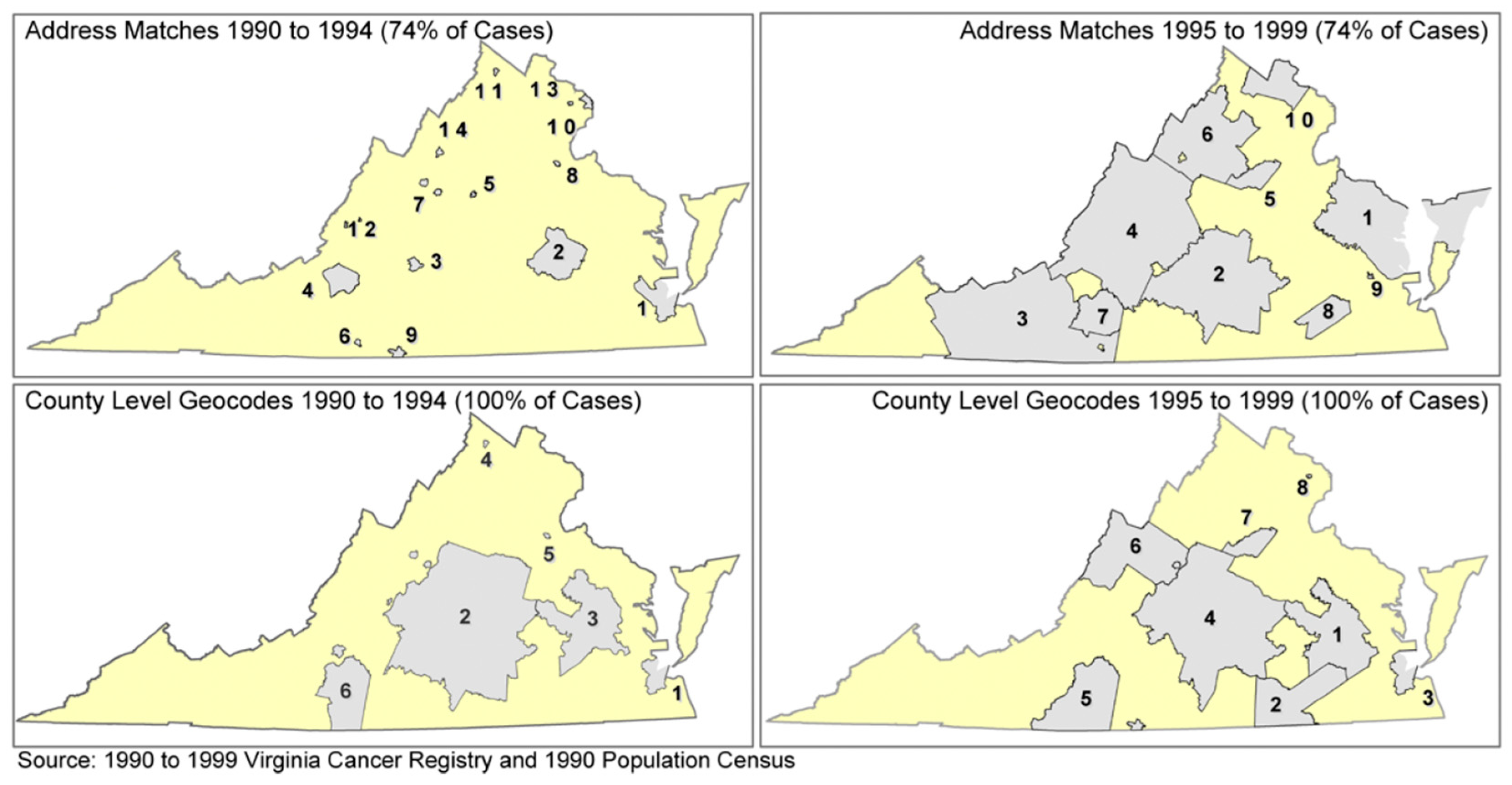
| Oliver M N et al. (2006) [41] | Virginia Cancer Registry (1990–1999) * | Census tract County | Mapping: Quantitative and qualitative Processing: Geocoding (74%–100%) and smoothing (headbanging) Analysis: Spatial autocorrelation (MEET), cluster identification (Spatial Scan Statistic) | Disparities in PCa incidence | Significant overall clustering with elevated incidence in eastern and central locations. |
| Gregorio DI et al. (2007) [42] | Connecticut Tumor Registry (1984–1998) | Exact patient address | Mapping: Qualitative Analysis: Cluster identification (Spatial Scan Statistic) | Disparities in PCa survival | Identification of three geographical clusters. Adjusting for age, tumor grade, stage, and race reduced clusters to one. PCa survival varies, only in part, according to place of residence. |
| Xiao H et al. (2007) [43] | Florida Cancer Data System (1990–2001) * | Census tract County | Mapping: Quantitative Processing: Geocoding (NA) | Disparities in PCa incidence, stage, and grade | Maps showing greatest racial disparities in incidence and late-stage PCa in the northern and central counties. |
| Hsu C E et al. (2007) [44] | Texas prostate cancer-specific death cases file (1980–2001) | County | Mapping: Qualitative Analysis: Cluster identification (Spatial Scan Statistic) | Disparities PCa mortality | Identification of statistically significant geographic counties with excess mortality rates for each of the racial groups studied and examination of those trends in function of time. |
| Hinrichsen VL (2009) [45] | Maryland Cancer Registry (1992–1997) | Census block groups | Processing: Geocoding (NA) Analysis: Spatial autocorrelation (Cuzick–Edwards’ k-NN, Global Moran’s I, MEET) | Disparities PCa stage and grade | For both grade and stage at diagnosis, Cuzick–Edwards’ k-NN and Moran’s I were very sensitive to the % of pop. parameter. For stage, all three tests showed that adjusting for individual and area level variables reduced clustering, but not entirely. |
| Meliker JR et al. (2009) [46] | Michigan Cancer Surveillance Program (1985–2002) | FHLD, SHLD Neighborhoods | Mapping: Quantitative Processing: Geocoding (91%) | Disparities in PCa survival | NHWs had significantly higher survival rates compared with AAs at the FHLD; however, in smaller geographic units (SHLD, neighborhoods), disparities diminished and disappeared. |
| Hébert JR (2010) [47] | South Carolina Cancer Registry (2001–2005) | DHEC Region | Mapping: Quantitative Processing: Geocoding (82%–100%) | Disparities in PCa MIR | Striking differences in MIR mapping between AAs and NHWs in the 8 DHEC regions examined. |
| Altekruse et al. (2010) [48] | State cancer registries of Tennessee, Alabama, Georgia, and Florida (1999–2001) * | Census tract | Mapping: Qualitative Analysis: Cluster identification (Spatial Scan Statistic) | Disparities in PCa incidence (localized) | Identification of statistically significant clusters. Higher incidence of localized disease in urban areas. |
| Goovaerts P et al. (2011) [49] | Florida Cancer Data System (1981–2007) | County | Mapping: Quantitative and qualitative Processing: Smoothing (Binomial Kriging) | Disparities in late stage PCa | Recent increase in the frequency of late-stage diagnosis in urban areas. The annual rate of decrease in late-stage diagnosis and the onset years for significant declines varied greatly among counties and racial groups. |
| Xiao H et al. (2011) [50] | Florida Cancer Data System (1996–2002) * | Census tract County | Mapping: Quantitative and qualitative Processing: Geocoding (NA), smoothing (Binomial Kriging) | Disparities in late-stage PCa | More counties had higher rates of late-stage diagnosis for AA men than for NHW men, and the location of these racial disparities changed with time. |
| Goovaerts P et al. (2012) [51] | Florida Cancer Data System (1981–2007) | County | Mapping: Quantitative and qualitative Processing: Smoothing (Binomial Kriging) Analysis: Cluster identification (spatially weighted cluster analysis) | Disparities in late-stage PCa | Geographical disparities were most widespread upon introduction of PSA screening. Spatially weighted cluster analysis resulted in spatially compact groups of counties with similar temporal trends. |
| Goovaerts P (2013) [52] | Florida Cancer Data System (1981–2007) | County | Mapping: Quantitative and qualitative Processing: Smoothing (Binomial Kriging) Analysis: Cluster identification (spatially weighted cluster analysis) | Disparities in late-stage PCa | A temporal trend in late-stage diagnosis suggests the existence of geographical disparities in the implementation and/or impact of the newly introduced PSA screening. |
| Wagner S et al. (2013) [53] | Georgia Comprehensive Cancer Registry (1998–2008) | Census tract County | Mapping: Quantitative and qualitative Analysis: Cluster identification (Getis-Ord-Gi and Spatial Scan Statistic) | Disparities in incidence and high grade or stage PCa | Pattern of higher incidence and more advanced disease found in northern and northwest central Georgia. Hotspot revealed six significant clusters of higher incidence for both races. When stratified by race, clusters among NHW and AA men were similar, although centroids were slightly shifted. |
| Gregorio DI (2013) [54] | Connecticut Tumor Registry (1994–1998) | Exact patient address | Mapping: Qualitative Analysis: Cluster identification (Spatial Scan Statistic) | PCa incidence | Two locations where incidence rates significantly exceeded the statewide level and two locations with significantly lower disease rates. Analysis adjusted for age and covariation of colorectal cancer incidence rates across the state accounted for all significant variations previously observed. |
| Goovaerts P (2015) [55] | Florida Cancer Data System (2001–2007) * | Census tract County | Mapping: Quantitative and qualitative Analysis: Geographically Weighted Regression | Disparities in late-stage PCa | Identification of locations where ORs for late-stage are higher/lower than the state level. |
| Wang M et al. (2017) [56] | Pennsylvania Cancer Registry (2000–2011) * | County | Mapping: Quantitative and qualitative Processing: Smoothing (Empirical Bayes) Analysis: Spatial autocorrelation (Global Moran’s I), cluster identification (Local Moran’s I) | Disparities in PCa incidence | Incidence of PCa among NHW males declined from 2000–2002 to 2009–2011, with significant variation across geographic regions. |
| Wang, M et al. (2020) [57] | Pennsylvania Cancer Registry (2004–2014) | Exact patient address | Mapping: Quantitative mapping Processing: Smoothing (Inverse Distance Weighting) | Disparities in aggressive PCa | Counties where AA population is lower than 5.3% have the highest odds of having the most aggressive forms of PCa in those AA men |
| Aghdam et al. (2020) [58] | Single institutional database (2008–2017) * | Zip code | Mapping: Qualitative | Disparities in PCa management | Travel distance did not prevent the uptake of SBRT for African American, elderly, or rural patients. |
| Georgantopoulos, P. et al. (2021) [59] | US Veterans Health Administration EMR (1999–2015) | ZCTA | Mapping: Quantitative and qualitative Analysis: Spatial autocorrelation (Global Moran’s I), cluster identification (Local Moran’s I) | Disparities in PCa MIR | Identification of spatial clusters of higher- or lower-than-expected MIRs by ZCTA. Two clusters of higher-than-expected MIRs were found in the upstate region. |
| Moore J. X. et al. (2022) [60] | CDC (1999–2019) | County | Mapping: Qualitative Processing: Smoothing (Empirical Bayes) Analysis: Cluster identification (Getis-Ord-Gi and Local Moran’s I) | Disparities in PCa mortality | Cancer mortality hotspots were heavily concentrated in three major areas in Georgia. Hotspot counties generally had a higher proportion of AA adults, older adult population, greater poverty, and more rurality |
| Aladuwaka et al. (2022) [61] | Alabama State Cancer Profile data (NA) * | County | Mapping: Quantitative and qualitative | Disparities in PCa incidence and mortality | Apparent socioeconomic disparity between the AA Belt and non-AA Belt counties of Alabama, which suggests that disparities in PCa incidence and mortality are strongly related to SES. |
| Tang C. et al. (2021) [62] | National Medicare Database (2011–2014) | Zip code County | Mapping: Quantitative and qualitative | Disparities in PCa management | Patient access was most limited for brachytherapy. Lower provider availability in rural areas, especially in western states. Heterogeneity in the access of definitive PCa treatment. Greater distance was associated with a decreased probability of treatment. |
| Study | Scanning Window Shape | Scanning Window Size | Clusters Delimited by Geopolitical Boundaries | Outcome |
|---|---|---|---|---|
| Jemal A et al. (2002) [38] | Circular | 0–50% of the total population at risk. | Yes (county) | PCa mortality |
| Klassen AC et al. (2005) [39] | Circular | 0–50% of the total population at risk. | No | PCa incidence, missing stage, and grade |
| DeChello LM et al. (2006) [40] | Circular | 0–50% of the total population at risk. | No | PCa incidence |
| Oliver M N et al. (2006) [41] | NA | NA (A Spatial Scan Statistic was used to evaluate raw counts). | NA (clusters not mapped) | PCa incidence |
| Gregorio DI et al. (2007) [42] | Circular | NA (varying sizes across the geography of the study area). | No | PCa survival |
| Hsu et al. (2007) [44] | NA | 50% and 90% of the study period. 50% of the population at risk. | Yes (county) | PCa mortality |
| Altekruse et al. (2010) [48] | Circular and elliptical | 0–50% of the total population at risk. | Yes (census tract) | PCa incidence (localized) |
| Wagner S et al. (2013) [53] | Circular | 50% spatial scanning window. | No | Incidence and high-grade or stage PCa |
| Gregorio DI (2013) [54] | Circular | NA (scanning circles at random locations and of varying sizes). | No | PCa incidence |
| GIS Application | Limitation(s)/Gap(s) | Proposed Recommendations(s) |
|---|---|---|
| Overall Scope |
|
|
| Mapping |
|
|
| Processing |
|
|
| Analysis |
|
|
| Method | Strengths | Weaknesses | Example of Recommended Application |
|---|---|---|---|
| Spatial Scan Statistic (SSS) |
|
| To detect significant circular or elliptical clusters of high PCa mortality within a specific region, accounting for the population at risk and considering varying cluster sizes |
| Local Moran’s I (LISA) |
|
| To identify statistically significant clusters of high or low PCa incidence rates, provide insight into neighboring observations, and understand spatial patterns of PCa incidence at smaller scales (census tracts, neighborhoods) |
| Hotspot Analysis (Getis-Ord Gi statistic) |
|
| To identify local hotspots or coldspots of PCa incidence within a specific geographic area, such as a county or a census tract |
| Geographically Weighted Regression (GWR) |
|
| To investigate the locally dynamic relationship between area-level characteristics (e.g., racial composition, socioeconomic status, availability of healthcare) and PCa outcomes (i.e., appropriate for multilevel analyses) |
Disclaimer/Publisher’s Note: The statements, opinions and data contained in all publications are solely those of the individual author(s) and contributor(s) and not of MDPI and/or the editor(s). MDPI and/or the editor(s) disclaim responsibility for any injury to people or property resulting from any ideas, methods, instructions or products referred to in the content. |
© 2024 by the author. Licensee MDPI, Basel, Switzerland. This article is an open access article distributed under the terms and conditions of the Creative Commons Attribution (CC BY) license (https://creativecommons.org/licenses/by/4.0/).
Share and Cite
El Khoury, C.J. Application of Geographic Information Systems (GIS) in the Study of Prostate Cancer Disparities: A Systematic Review. Cancers 2024, 16, 2715. https://doi.org/10.3390/cancers16152715
El Khoury CJ. Application of Geographic Information Systems (GIS) in the Study of Prostate Cancer Disparities: A Systematic Review. Cancers. 2024; 16(15):2715. https://doi.org/10.3390/cancers16152715
Chicago/Turabian StyleEl Khoury, Christiane J. 2024. "Application of Geographic Information Systems (GIS) in the Study of Prostate Cancer Disparities: A Systematic Review" Cancers 16, no. 15: 2715. https://doi.org/10.3390/cancers16152715