
Multi-Modal MR Image Segmentation Strategy for Brain Tumors Based on Domain Adaptation

Abstract

1. Introduction
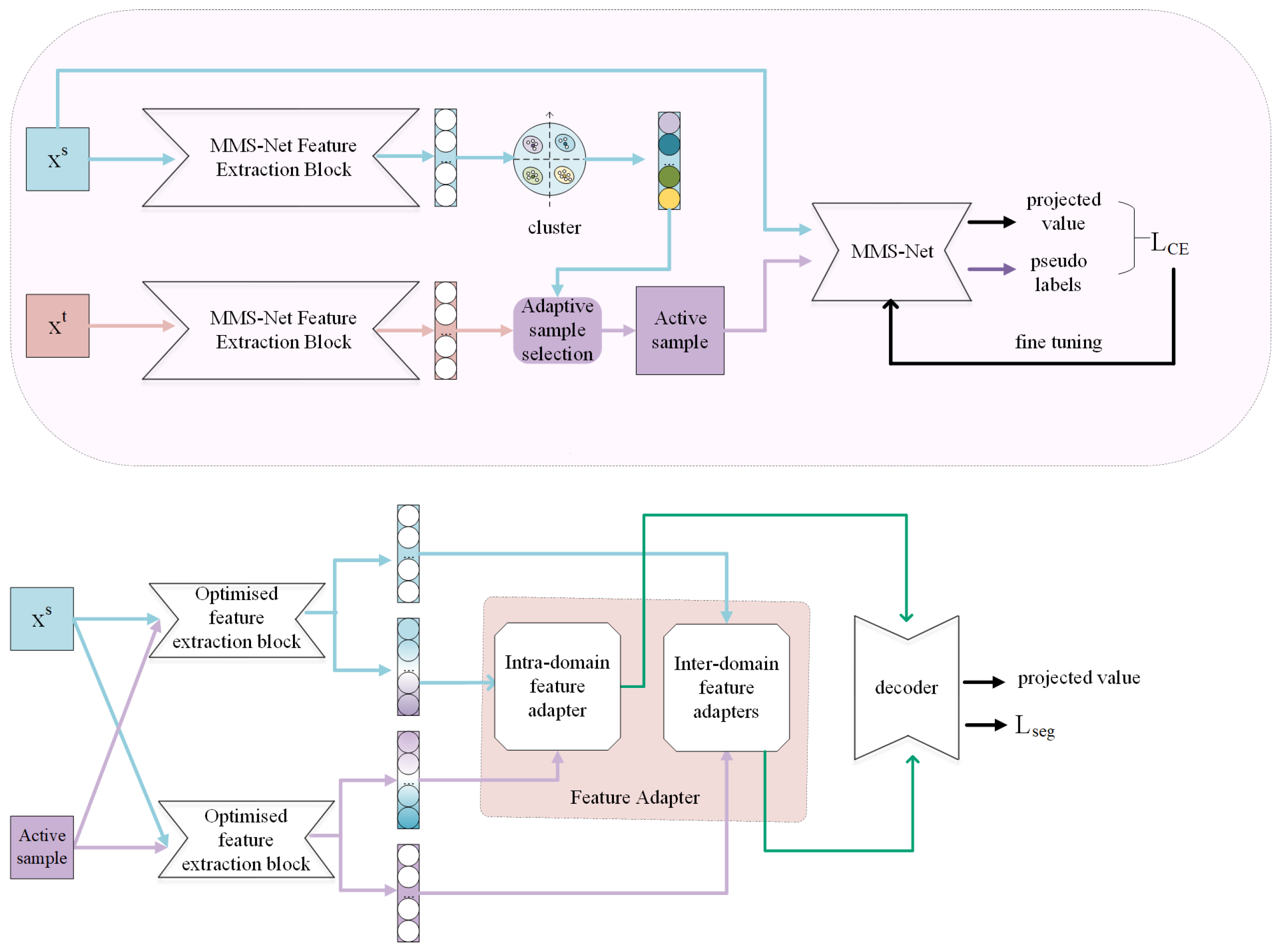
- Targets with different modal features of the source domain are derived using clustering methods in the pre-training stage.
- For each target, samples with the strongest complementarity to the source domain are identified in the target domain data, and the corresponding pseudo labels are produced and applied to train the network.
- Feature alignment is performed using a feature adapter; the feature adapter is a modular structure that learns to align features from source- and target-domain images.
- To improve the generalization ability of the network, a network structure is designed that is sensitive to the source- and target-domain images, making it better adapted to the data distribution in different domains.
2. Related Work
2.1. Relevant Research
2.2. Relevant Knowledge
- Domain shiftDomain shift stems from the machine learning model, trained on a dataset, displaying reduced performance in different datasets. This phenomenon is derived from variations in the underlying data distributions, such as differences in features, labels, or sample distributions.The domain shift problem occurs even when deep convolutional neural networks are trained on large image datasets, which is a challenge in the era of the rapid development of deep learning technology. In domains such as medical images, the domain shift problem needs to be solved. The DA technique is used to solve the domain shift problem during data migration.
- Domain GeneralizationDomain generalization investigates the problems in which, in the case of there being only source domain data, multiple source domain data with different distributions can be used to train and learn a model with strong generalizability, which achieves better performance on unknown target domains. The main difference between the domain generalization problem and the domain adaptation problem is that in domain generalization the target domain is unknown and only the data of the source domain are trained. In contrast, in domain adaptation, the target domain and source domain data are utilized in the training. The advantage of domain generalization is that models that require a single training can be applied to diverse scenarios. Using MR and CT as examples, a great difference is observed in the appearance between the images acquired by these two methods. Training two respective segmentation models on CT or MR alone and followed by the adoption of these two models to segment a common set of CT images, called ‘CT to CT’ and ‘MR to CT’, respectively, leads to the appearance of the segmentation model trained on MR images alone. The model trained on MR images alone does not generalize well to CT images directly, or the model trained on CT images alone does not generalize well to MR images directly.
- Negative migrationThe main focus of DA is to learn from the knowledge of the source domain to perform well on the target task. However, in some cases, DA may face the following challenges: (1) the tasks in the source and target domains are not related or similar; (2) the feature space or data distribution of the data in the source and target domains are different; (3) the trained model cannot be applied to the source and target domains, leading to negative migration. In medical imaging, data from different modalities exhibit specific distributions, and sometimes it is necessary to encode the appearance, shape, and context simultaneously to eliminate distributional differences. Negative migration is a major challenge during the application of domain adaptation in medical tasks.
3. Proposed Method
3.1. Network Framework
3.2. Adaptive Generation of Pseudo-Labels
3.2.1. Generate Source Domain Targets
3.2.2. Adaptive Sample Selection
3.2.3. Generation of Pseudo-Labels
| Algorithm 1 Adaptive sample selection |
|
| Algorithm 2 Pseudo-Label Generation Algorithm |
|
3.3. Feature Adapter
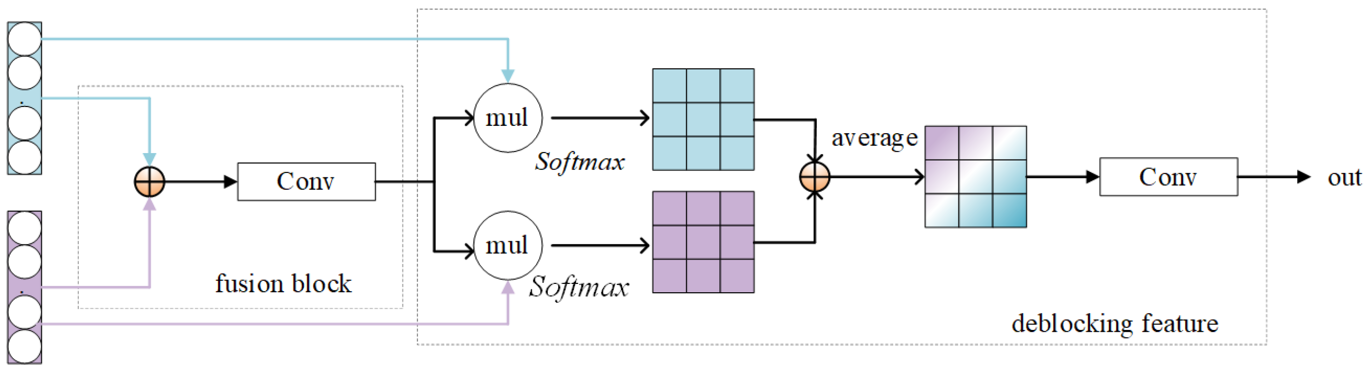
3.3.1. Inter-Domain Feature Adapters
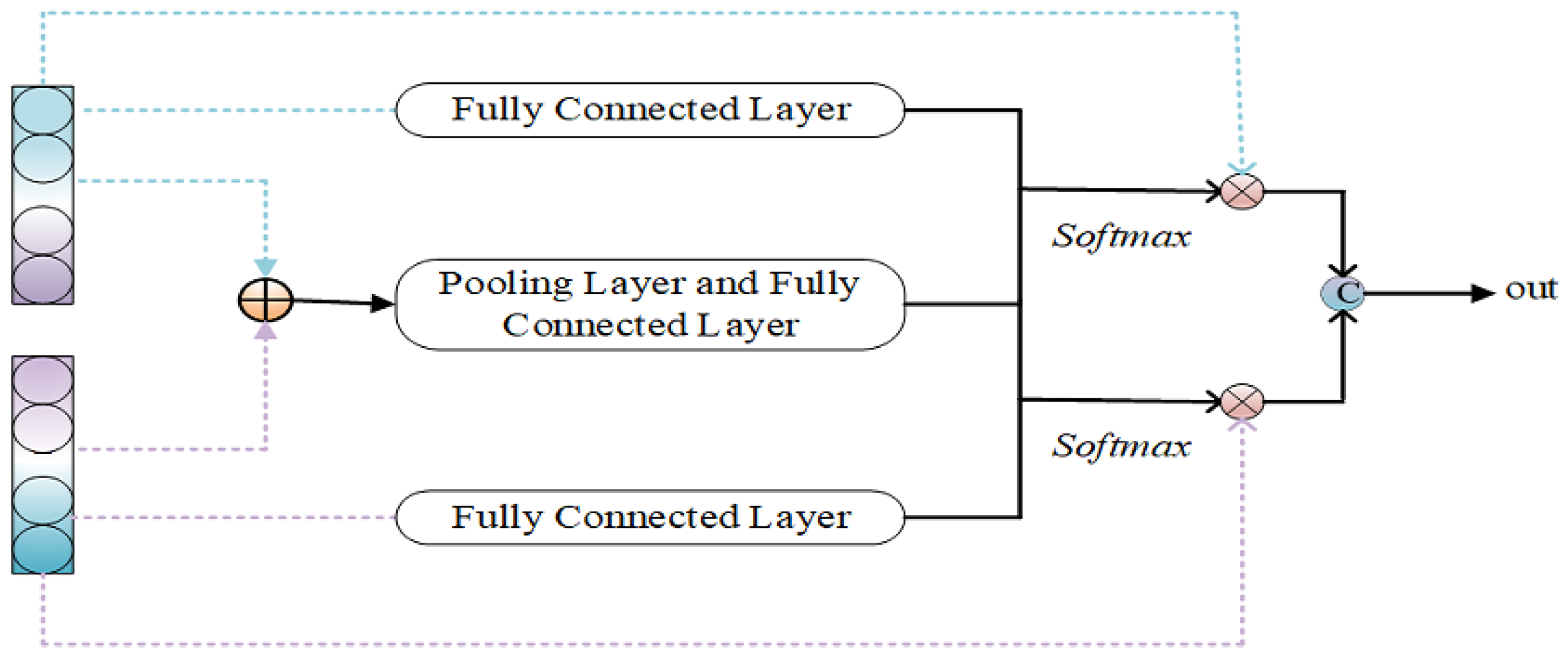
3.3.2. Intra-Domain Feature Adapters
4. Experiment
4.1. Dataset
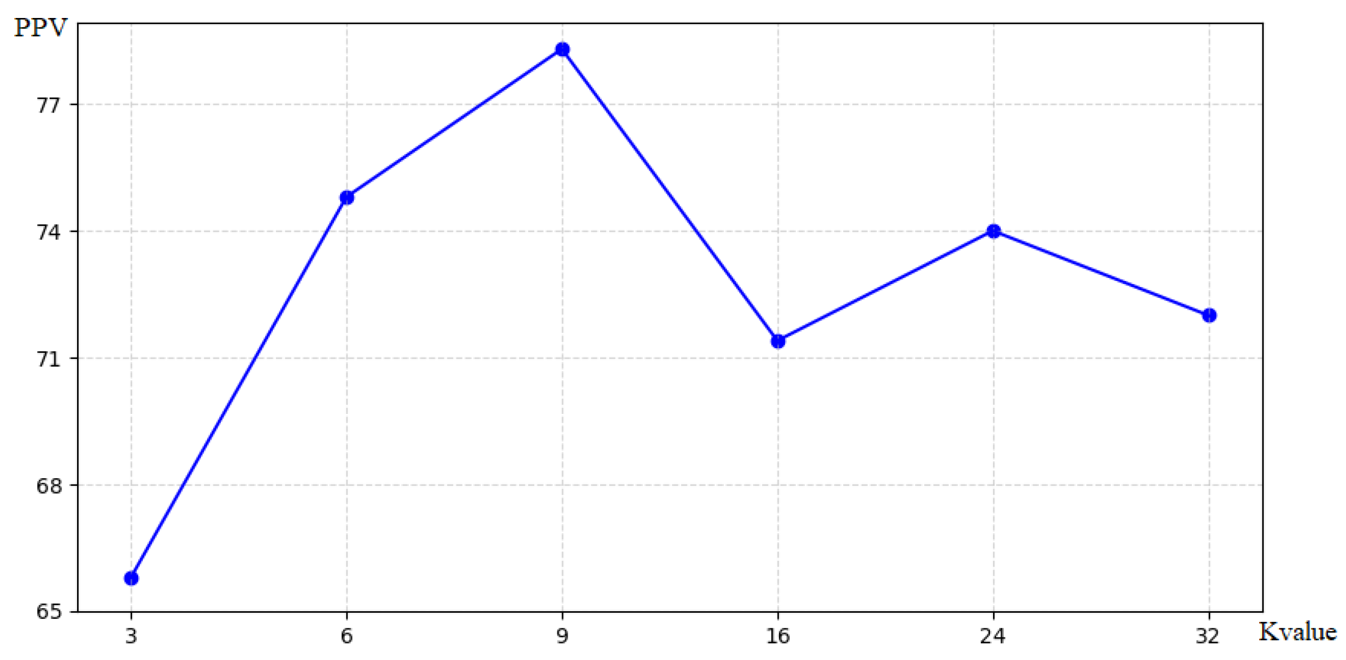
4.2. K-Value Setting
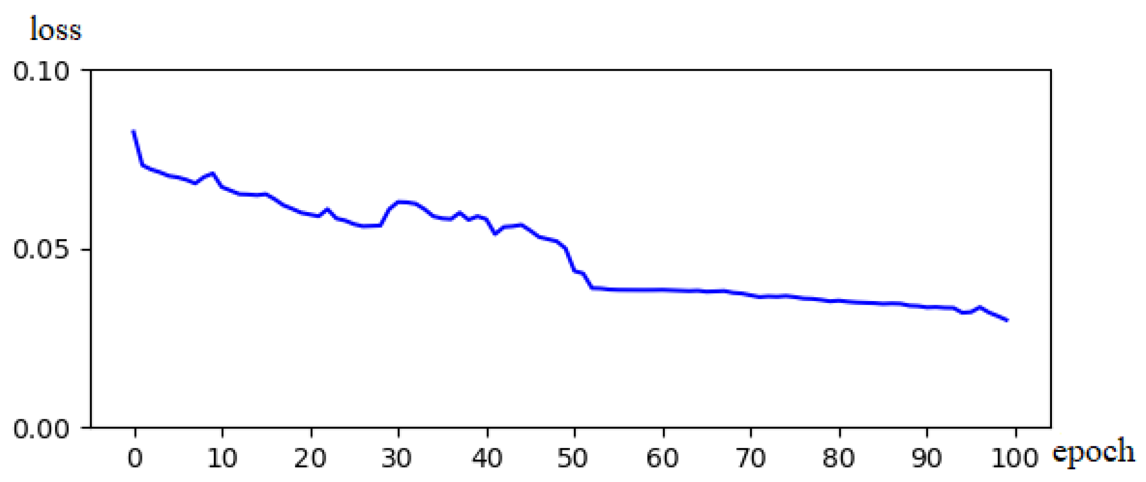
4.3. Loss Function
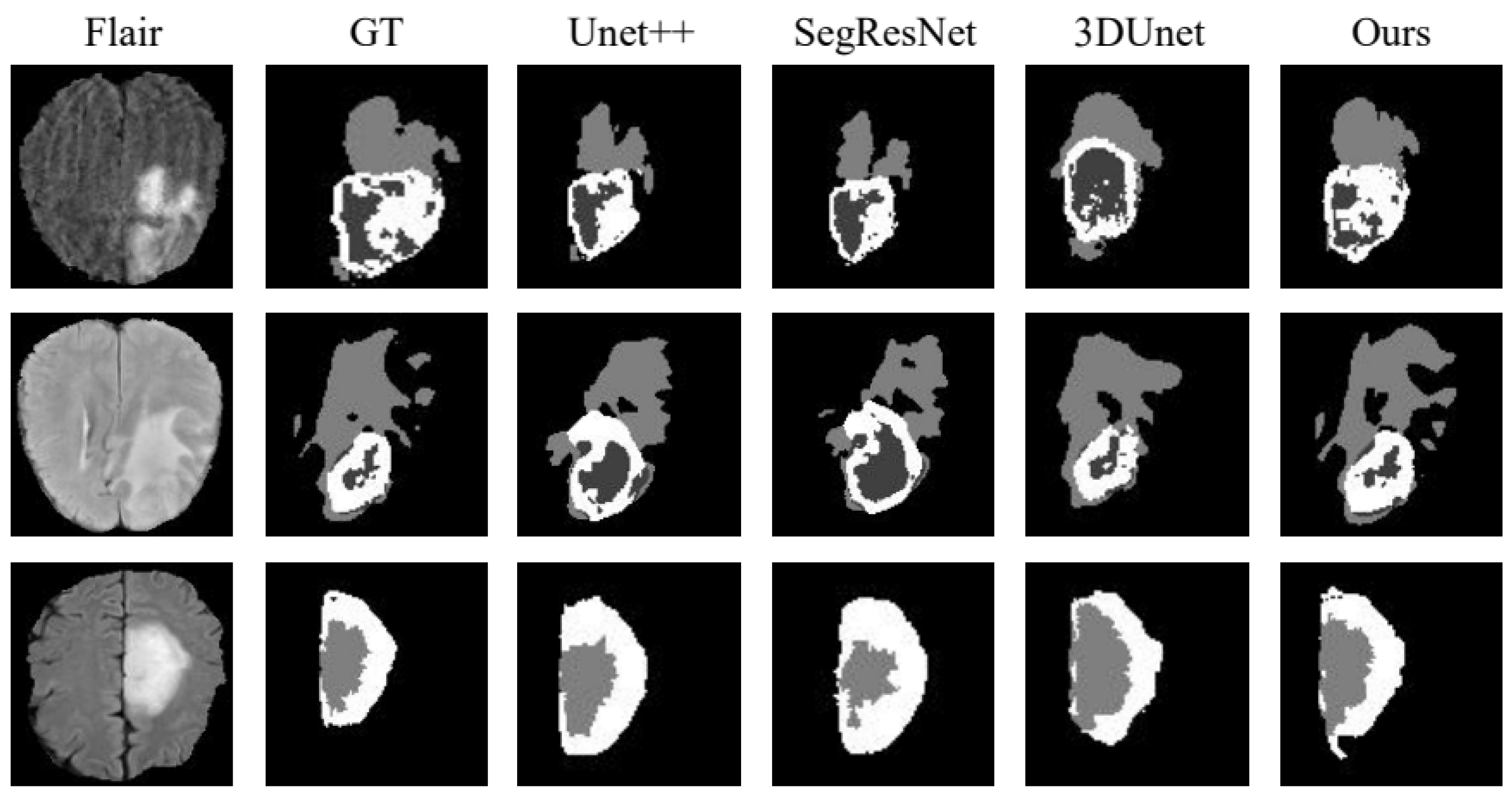
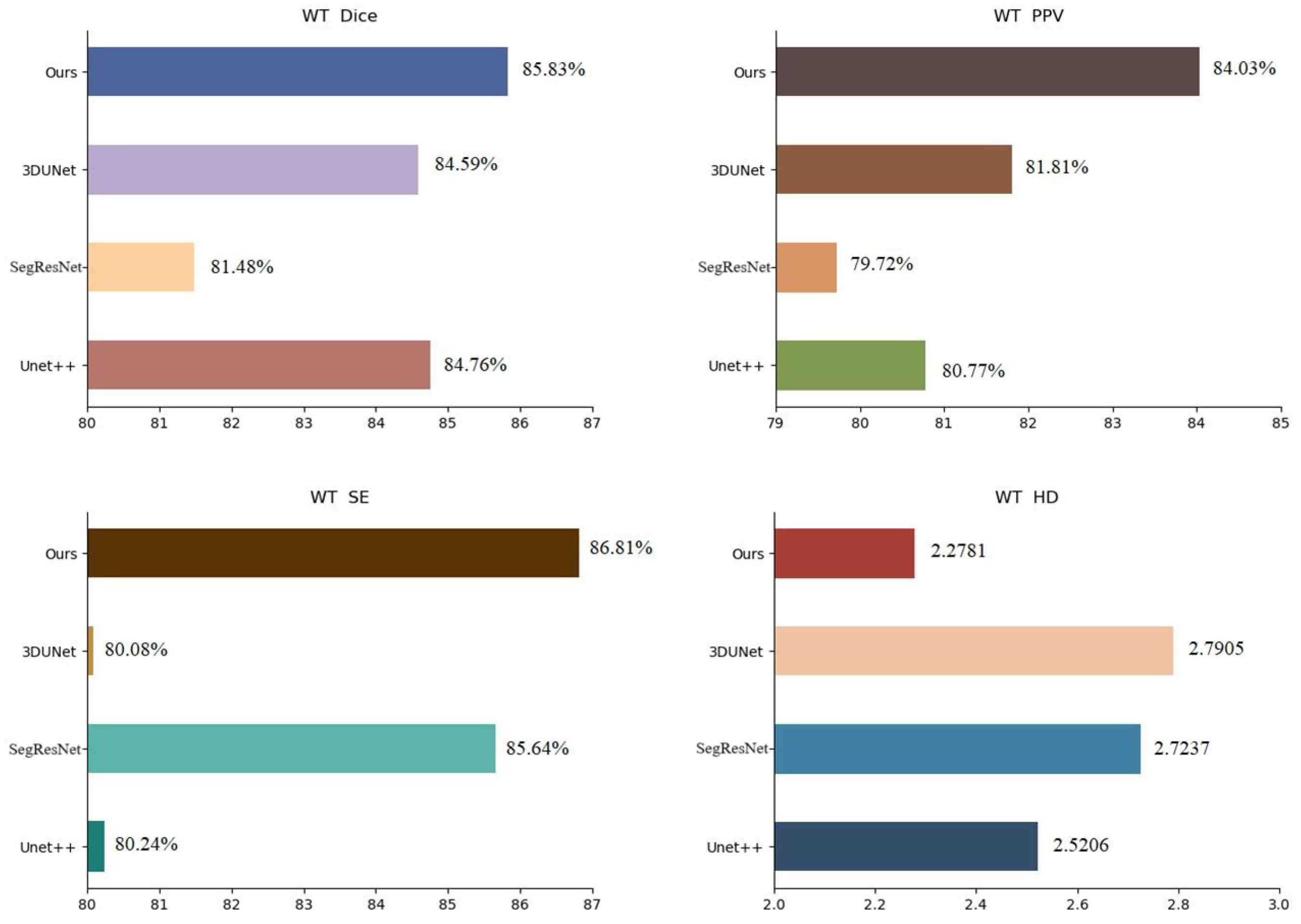
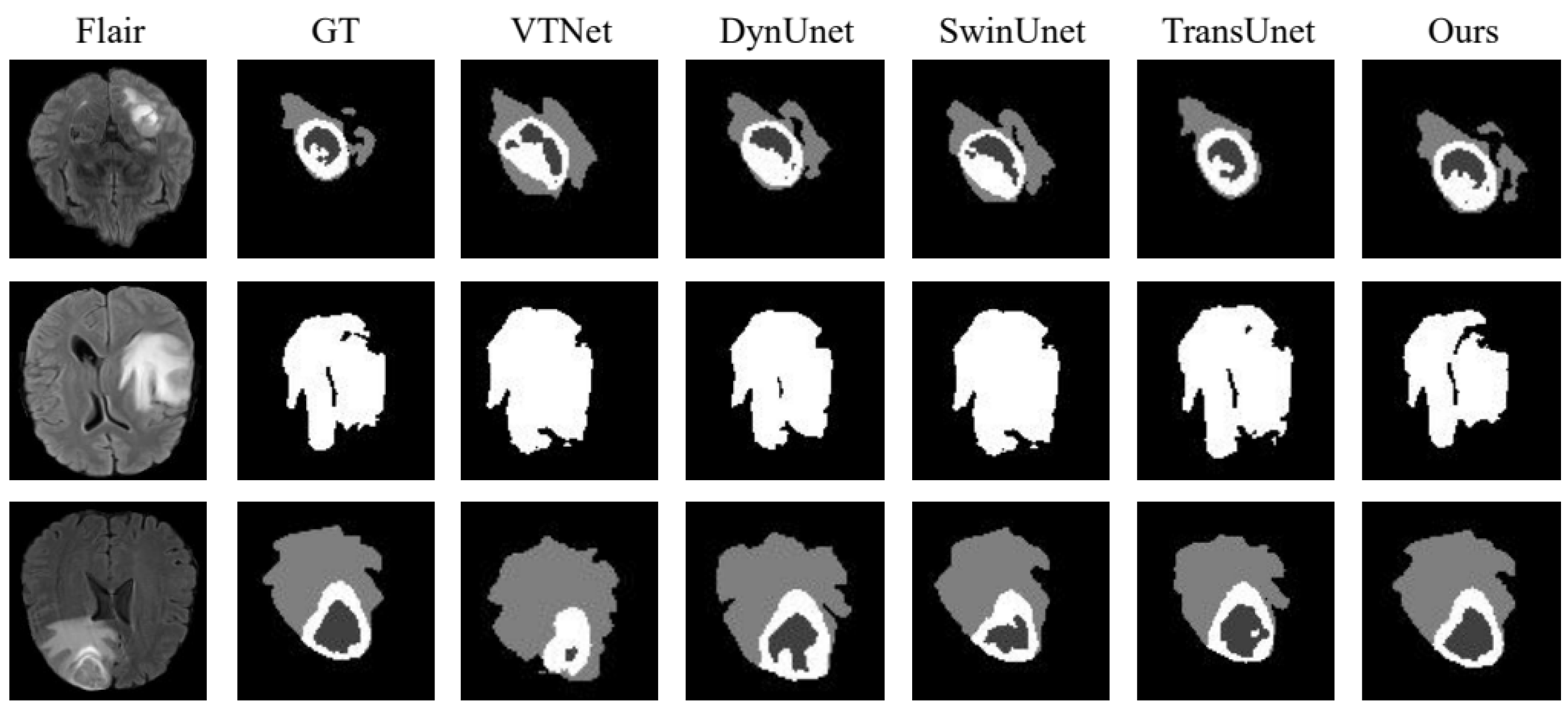
4.4. Comparison of Similar Methods
5. Discussion
6. Summary
Author Contributions
Funding
Institutional Review Board Statement
Informed Consent Statement
Data Availability Statement
Conflicts of Interest
References
- Biratu, E.S.; Schwenker, F.; Ayano, Y.M.; Debelee, T.G. A survey of brain tumor segmentation and classification algorithms. J. Imaging 2021, 7, 179. [Google Scholar] [CrossRef] [PubMed]
- Pan, S.J.; Yang, Q. A survey on transfer learning. IEEE Trans. Knowl. Data Eng. 2010, 22, 1345–1359. [Google Scholar] [CrossRef]
- Guo, H.; Pasunuru, R.; Bansal, M. Multi-source domain adaptation for text classification via distance-net bandits. AAAI Conf. Artif. Intell. 2020, 34, 7830–7838. [Google Scholar]
- Zou, H.; Yang, J.; Wu, X. Unsupervised energy-based adversarial domain adaptation for cross-domain text classification. In Proceedings of the Findings of the Association for Computational Linguistics, Online, 1–6 August 2021; pp. 1208–1218. [Google Scholar]
- Xu, L.; Gong, H.; Zhong, Y.; Wang, F.; Wang, S.; Lu, L.; Ding, J.; Zhao, C.; Tang, W.; Xu, J. Real-time monitoring of manual acupuncture stimulation parameters based on domain adaptive 3D hand pose estimation. Biomed. Signal Process. Control 2023, 83, 104681. [Google Scholar] [CrossRef]
- Zhang, X.; Ji, J.; Wang, L.; He, Z.; Liu, S. Review of video-based identification and detection methods of abnormal human behavior. Control Decis. Mak. 2022, 37, 14–27. [Google Scholar]
- Chen, Y.; Liu, Q.; Peng, D. A component-aware adaptive algorithm for pose estimation. Comput. Eng. 2018, 44, 263–270. [Google Scholar]
- Kiran, M.; Pedersoli, M.; Dolz, J.; Blais-Morin, L.A.; Granger, E. Incremental multi-target domain adaptation for object detection with efficient domain transfer. Pattern Recognit. 2022, 129, 108771. [Google Scholar]
- Oza, P.; Sindagi, V.A.; Sharmini, V.V.; Patel, V.M. Unsupervised domain adaptation of object detectors: A survey. IEEE Trans. Pattern Anal. Mach. Intell. 2024, 46, 4018–4040. [Google Scholar] [CrossRef] [PubMed]
- Zhang, D.; Ye, M.; Liu, Y.; Xiong, L.; Zhou, L. Multi-source unsupervised domain adaptation for object detection. Inf. Fusion 2022, 78, 138–148. [Google Scholar] [CrossRef]
- Jie, G. Research on Domain Adaptation and Semantic Association in Video Concept Detection; Beijing Jiaotong University: Beijing, China, 2016. [Google Scholar]
- Wachinger, C.; Reuter, M.; Initiative, A.D.N. Domain adaptation for Alzheimer’s disease diagnostics. Neuroimage 2016, 139, 470–479. [Google Scholar] [CrossRef]
- Goetz, M.; Weber, C.; Binczyk, F.; Polanska, J.; Tarnawski, R.; Bobek-Billewicz, B.; Koethe, U.; Kleesiek, J.; Stieltjes, B.; Maier-Hein, K.H. DALSA: Domain adaptation for supervised learning from sparsely annotated MR images. IEEE Trans. Med. Imaging 2015, 35, 184–196. [Google Scholar] [CrossRef] [PubMed]
- Chen, C.; Dou, Q.; Chen, H.; Qin, J.; Heng, P.A. Synergistic image and feature adaptation: Towards cross-modality domain adaptation for medical image segmentation. In Proceedings of the AAAI Conference on Artificial Intelligence, Honolulu, HI, USA, 27 January–1 February 2019; Volume 33, pp. 865–872. [Google Scholar]
- Han, X.; Qi, L.; Yu, Q.; Zhou, Z.; Zheng, Y.; Shi, Y.; Gao, Y. Deep symmetric adaptation network for cross-modality medical image segmentation. IEEE Trans. Med. Imaging 2021, 41, 121–132. [Google Scholar] [CrossRef] [PubMed]
- Vesal, S.; Ravikumar, N.; Maier, A. Automated multi-sequence cardiac MRI segmentation using supervised domain adaptation. In Proceedings of the Statistical Atlases and Computational Models of the Heart, Multi-Sequence CMR Segmentation, CRT-EPiggy and LV Full Quantification Challenges, Shenzhen, China, 13 October 2019; Springer: Berlin/Heidelberg, Germany, 2020; pp. 300–308. [Google Scholar]
- Kushibar, K.; Valverde, S.; Gonzalez-Villa, S.; Bernal, J.; Cabezas, M.; Oliver, A.; Llado, X. Supervised domain adaptation for automatic sub-cortical brain structure segmentation with minimal user interaction. Sci. Rep. 2019, 9, 6742. [Google Scholar] [CrossRef] [PubMed]
- Gu, Y.; Ge, Z.; Bonnington, C.P.; Zhou, J. Progressive transfer learning and adversarial domain adaptation for cross-domain skin disease classification. IEEE J. Biomed. Health Inform. 2019, 24, 1379–1393. [Google Scholar] [CrossRef]
- Kaur, B.; Lemaître, P.; Mehta, R.; Sepahvand, N.M.; Precup, D.; Arnold, D.; Arbel, T. Improving pathological structure segmentation via transfer learning across diseases. In Proceedings of the Domain Adaptation and Representation Transfer and Medical Image Learning with Less Labels and Imperfect Data, Shenzhen, China, 13 and 17 October 2019; Springer: Berlin/Heidelberg, Germany, 2019; pp. 90–98. [Google Scholar]
- Kamphenkel, J.; Jäger, P.F.; Bickelhaupt, S.; Laun, F.B.; Lederer, W.; Daniel, H.; Kuder, T.A.; Delorme, S.; Schlemmer, H.P.; König, F.; et al. Domain adaptation for deviating acquisition protocols in CNN-based lesion classification on diffusion-weighted MR images. In Image Analysis for Moving Organ, Breast, and Thoracic Images; Springer: Berlin/Heidelberg, Germany, 2018; pp. 73–80. [Google Scholar]
- Gao, Y.; Zhang, Y.; Cao, Z.; Guo, X.; Zhang, J. Decoding brain states from fMRI signals by using unsupervised domain adaptation. IEEE J. Biomed. Health Inform. 2019, 24, 1677–1685. [Google Scholar] [CrossRef] [PubMed]
- Bateson, M.; Kervadec, H.; Dolz, J.; Lombaert, H.; Ayed, I.B. Constrained domain adaptation for segmentation. In Proceedings of the Medical Image Computing and Computer Assisted Intervention—MICCAI 2019, Shenzhen, China, 13–17 October 2019; Springer: Berlin/Heidelberg, Germany, 2019; pp. 326–334. [Google Scholar]
- Sheng, X.; Zhang, Y. Multimodal brain tumour MR image segmentation by incorporating attention mechanism. J.-Comput.-Aided Des. Graph. 2023, 35, 1429–1438. [Google Scholar]
- MacQueen, J. Some methods for classification and analysis of multivariate observations. In Proceedings of the 5th Berkeley Symposium on Mathematical Statistics and Probability, Berkeley, CA, USA, 21 June–18 July 1965; p. 281. [Google Scholar]
- Zhou, Z.; Siddiquee, M.M.R.; Tajbakhsh, N.; Liang, J. Unet++: A nested u-net architecture for medical image segmentation. In Proceedings of the Deep Learning in Medical Image Analysis and Multimodal Learning for Clinical Decision Support, Granada, Spain, 20 September 2018; Springer: Berlin/Heidelberg, Germany, 2018; pp. 3–11. [Google Scholar]
- Myronenko, A. 3D MRI brain tumor segmentation using autoencoder regularization. In Brain-Lesion: Glioma, Multiple Sclerosis, Stroke and Traumatic Brain Injuries; Springer: Berlin/Heidelberg, Germany, 2019; pp. 311–320. [Google Scholar]
- Çiçek, Ö.; Abdulkadir, A.; Lienkamp, S.S.; Brox, T.; Ronneberger, O. 3D U-Net: Learning dense volumetric segmentation from sparse annotation. In Proceedings of the Medical Image Computing and Computer-Assisted Intervention–MICCAI 2016: 19th International Conference, Athens, Greece, 17–21 October 2016; Proceedings, Part II 19. Springer: Berlin/Heidelberg, Germany, 2016; pp. 424–432. [Google Scholar]
- Milletari, F.; Navab, N.; Ahmadi, S.A. V-net: Fully convolutional neural networks for volumetric medical image segmentation. In Proceedings of the 2016 Fourth International Conference on 3D Vision (3DV), Stanford, CA, USA, 25–28 October 2016; IEEE: Piscataway, NJ, USA, 2016; pp. 565–571. [Google Scholar]
- Futrega, M.; Milesi, A.; Marcinkiewicz, M.; Ribalta, P. Optimized U-Net for brain tumor segmentation. In Brainlesion: Glioma, Multiple Sclerosis, Stroke and Traumatic Brain Injuries; Springer: Berlin/Heidelberg, Germany, 2022; pp. 15–29. [Google Scholar]
- Cao, H.; Wang, Y.; Chen, J.; Jiang, D.; Zhang, X.; Tian, Q.; Wang, M. Swin-unet: Unet-like pure transformer for medical image segmentation. In Proceedings of the Computer Vision—ECCV 2022 Workshops, Online, 23 October 2022; Springer: Berlin/Heidelberg, Germany, 2023; pp. 205–218. [Google Scholar]
- Chen, J.; Lu, Y.; Yu, Q.; Luo, X.; Adeli, E.; Wang, Y.; Lu, L.; Yuille, A.L.; Zhou, Y. Transunet: Transformers make strong encoders for medical image segmentation. arXiv 2021, arXiv:2102.04306. [Google Scholar]

| Method | References | Assignment | Datasets | Image Types |
|---|---|---|---|---|
| Instance Weighting | Wachinger et al. [12] | AD Classification | ADNI/AIBL/CADDementia | MR |
| Goetz et al. [13] | Tumor Segmentation | BraTs | MR | |
| Feature Transformation | Chen et al. [14] | Cardiac Segmentation | Heart 2017 | CT/MR |
| Han et al. [15] | Multiorgan Segmentation | Heart/BraTs | MR | |
| Supervised Learning | Vesal et al. [16] | Cardiac Segmentation | Heart 2019 | MR |
| Kushibar et al. [17] | Tumor Segmentation | Miccai 2012/IBSR | MR | |
| Gu et al. [18] | Disease Classification | HAM/MoleMAp | / | |
| Kaur et al. [19] | Tumor Segmentation | BraTs | MR | |
| Unsupervised Learning | Kamphenkel et al. [20] | Breast Cancer Classification | / | MR |
| Gao et al. [21] | Brain Activity Classification | HCP | fMR | |
| Bateson et al. [22] | Intervertebral Disc Segmentation | MICCAI2018/IVDM3Seg | MR |
| Datasets | Resolution | Number | Role |
|---|---|---|---|
| BraTs18 | 285 | Training set, source domain | |
| BraTs19 | 335 | Test set, target domain | |
| BraTs21 | 1251 | Target domain |
| Evaluation Metrics | DC/% | PPV/% | SE/% | HD | ||||||||
|---|---|---|---|---|---|---|---|---|---|---|---|---|
| WT | TC | ET | WT | TC | ET | WT | TC | ET | WT | TC | ET | |
| Unet++ [25] | 84.76 | 81.23 | 79.88 | 80.77 | 79.95 | 81.49 | 80.24 | 78.52 | 79.80 | 2.5206 | 2.0684 | 2.4125 |
| SegResNet [26] | 81.48 | 80.49 | 78.69 | 79.72 | 80.59 | 78.52 | 85.64 | 83.41 | 77.58 | 2.7237 | 2.6606 | 2.6189 |
| 3DUNet [27] | 84.59 | 83.27 | 82.73 | 81.81 | 78.97 | 79.99 | 80.08 | 81.36 | 79.42 | 2.7905 | 2.5123 | 2.6131 |
| ours | 85.83 | 86.85 | 84.66 | 84.03 | 85.69 | 82.91 | 86.81 | 85.84 | 81.47 | 2.2781 | 1.9164 | 2.3109 |
| Evaluation Metrics | DC/% | PPV/% | SE/% | HD | ||||||||
|---|---|---|---|---|---|---|---|---|---|---|---|---|
| WT | TC | ET | WT | TC | ET | WT | TC | ET | WT | TC | ET | |
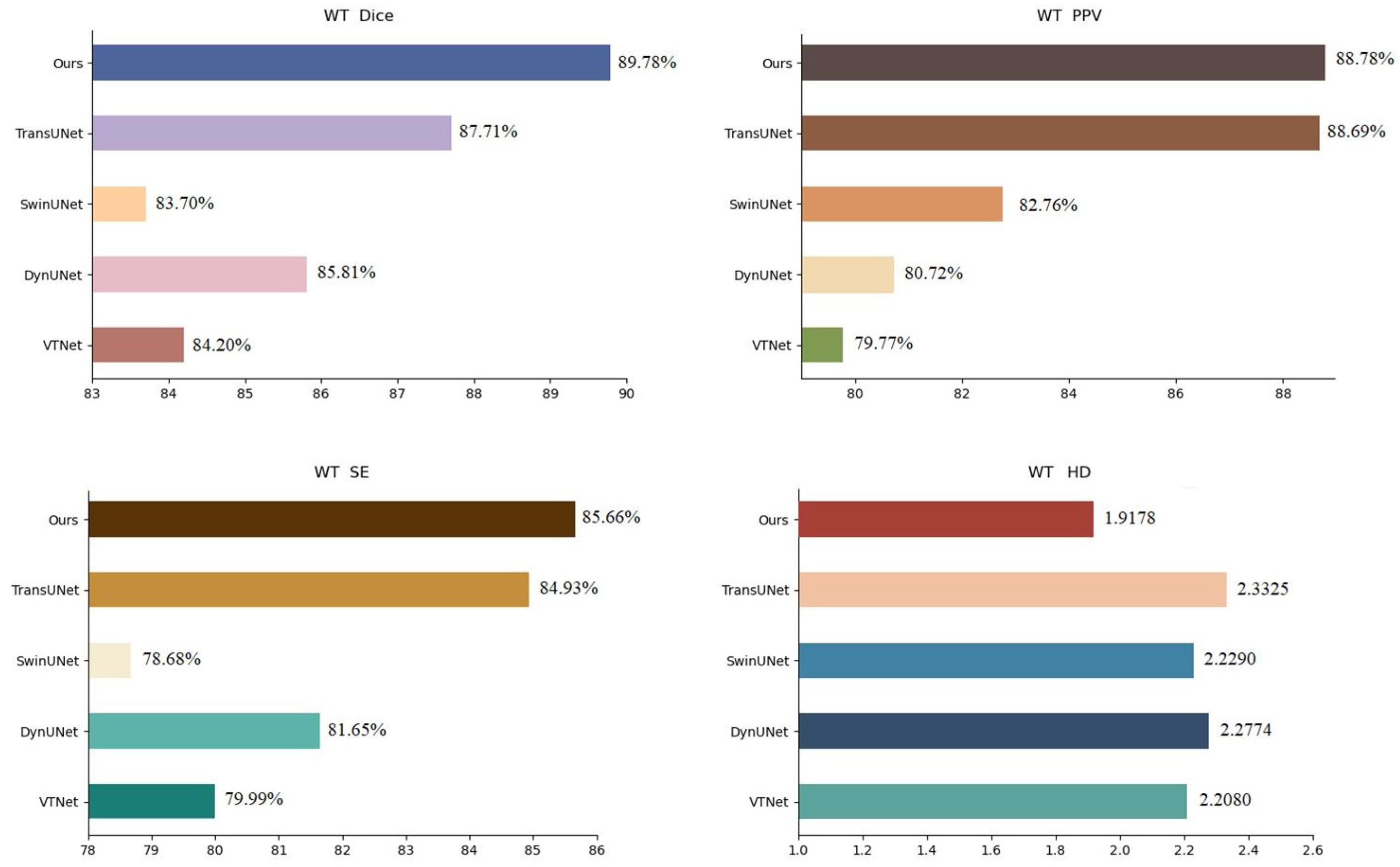
| VTNet [28] | 84.20 | 80.51 | 78.20 | 79.77 | 81.79 | 78.81 | 79.99 | 80.96 | 78.86 | 2.2080 | 2.1569 | 2.0526 |
| DynUNet [29] | 85.81 | 83.87 | 82.94 | 80.72 | 78.89 | 79.74 | 81.65 | 80.08 | 81.24 | 2.2774 | 2.5206 | 2.1189 |
| SwinUnet [30] | 83.70 | 81.85 | 80.92 | 82.76 | 80.77 | 80.75 | 78.68 | 79.54 | 77.82 | 2.2290 | 2.1236 | 2.5131 |
| TransUnet [31] | 87.71 | 88.82 | 87.96 | 88.69 | 85.43 | 82.42 | 84.93 | 83.47 | 84.08 | 2.3325 | 1.8155 | 2.0136 |
| Ours | 89.78 | 87.89 | 84.05 | 88.78 | 85.91 | 84.85 | 85.66 | 83.69 | 85.96 | 1.9178 | 2.2164 | 2.0109 |
Disclaimer/Publisher’s Note: The statements, opinions and data contained in all publications are solely those of the individual author(s) and contributor(s) and not of MDPI and/or the editor(s). MDPI and/or the editor(s) disclaim responsibility for any injury to people or property resulting from any ideas, methods, instructions or products referred to in the content. |
© 2024 by the authors. Licensee MDPI, Basel, Switzerland. This article is an open access article distributed under the terms and conditions of the Creative Commons Attribution (CC BY) license (https://creativecommons.org/licenses/by/4.0/).
Share and Cite
Yang, Q.; Jing, R.; Mu, J. Multi-Modal MR Image Segmentation Strategy for Brain Tumors Based on Domain Adaptation. Computers 2024, 13, 347. https://doi.org/10.3390/computers13120347
Yang Q, Jing R, Mu J. Multi-Modal MR Image Segmentation Strategy for Brain Tumors Based on Domain Adaptation. Computers. 2024; 13(12):347. https://doi.org/10.3390/computers13120347
Chicago/Turabian StyleYang, Qihong, Ruijun Jing, and Jiliang Mu. 2024. "Multi-Modal MR Image Segmentation Strategy for Brain Tumors Based on Domain Adaptation" Computers 13, no. 12: 347. https://doi.org/10.3390/computers13120347
APA StyleYang, Q., Jing, R., & Mu, J. (2024). Multi-Modal MR Image Segmentation Strategy for Brain Tumors Based on Domain Adaptation. Computers, 13(12), 347. https://doi.org/10.3390/computers13120347