
Human Emotion Recognition Based on Spatio-Temporal Facial Features Using HOG-HOF and VGG-LSTM


Abstract
1. Introduction
2. Related Works
2.1. Dynamic Texture-Based Methods
2.2. Deep Learning Methods
2.3. Transfer Learning Methods
Result and Limitation of Existence Methods
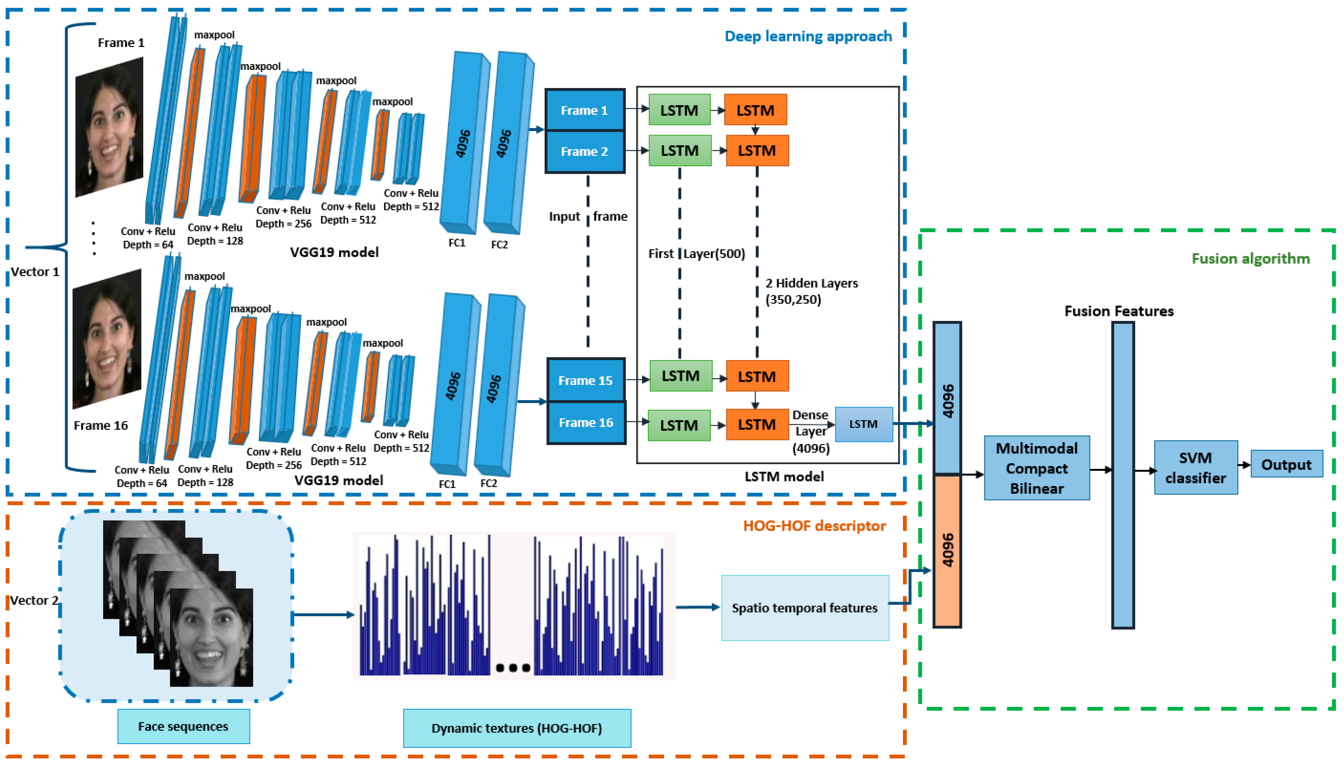
3. The Proposed Approach
3.1. Deep Learning Part
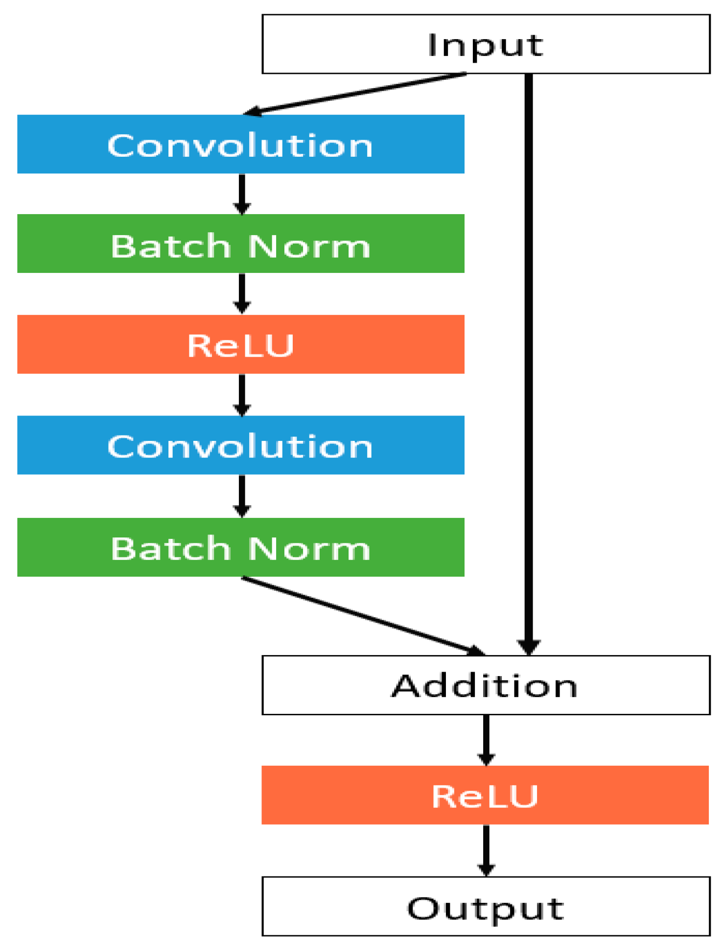
3.1.1. ResNet
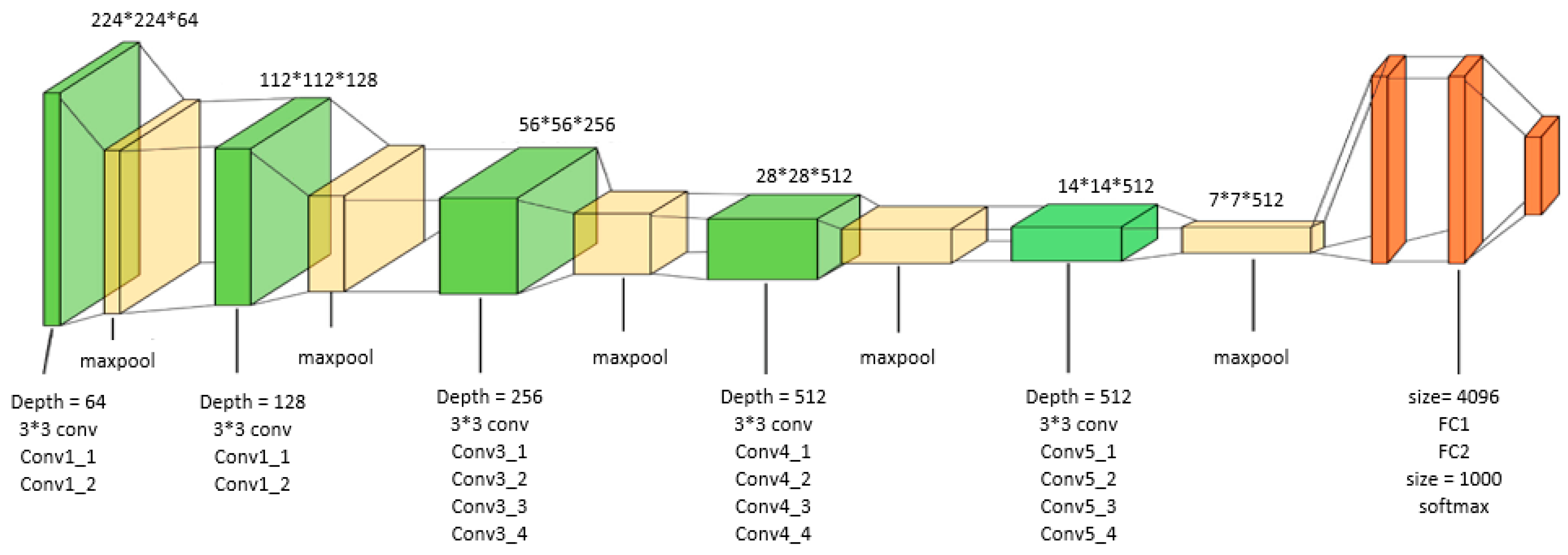
3.1.2. VGG19
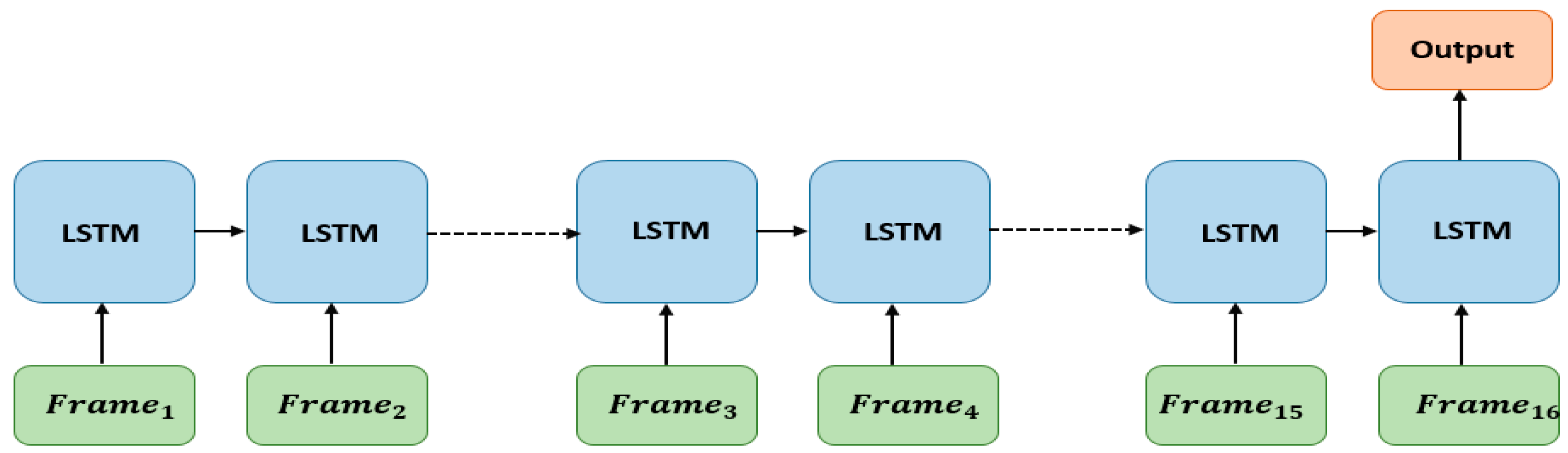
3.1.3. LSTM
- is the input at time step
- is the output of the previous time step.
- ,, and are the weight matrix and bias vector for the input gate, respectively.
- is the sigmoid activation function.
- , and are the weight matrix and bias vector for the forget gate, respectively.
- , and are the weight matrix and bias vector for updating the cell state.
- is the cell state from the previous time step.
- , and are the weight matrix and bias vector for updating the cell state.
3.2. HOG-HOF Part
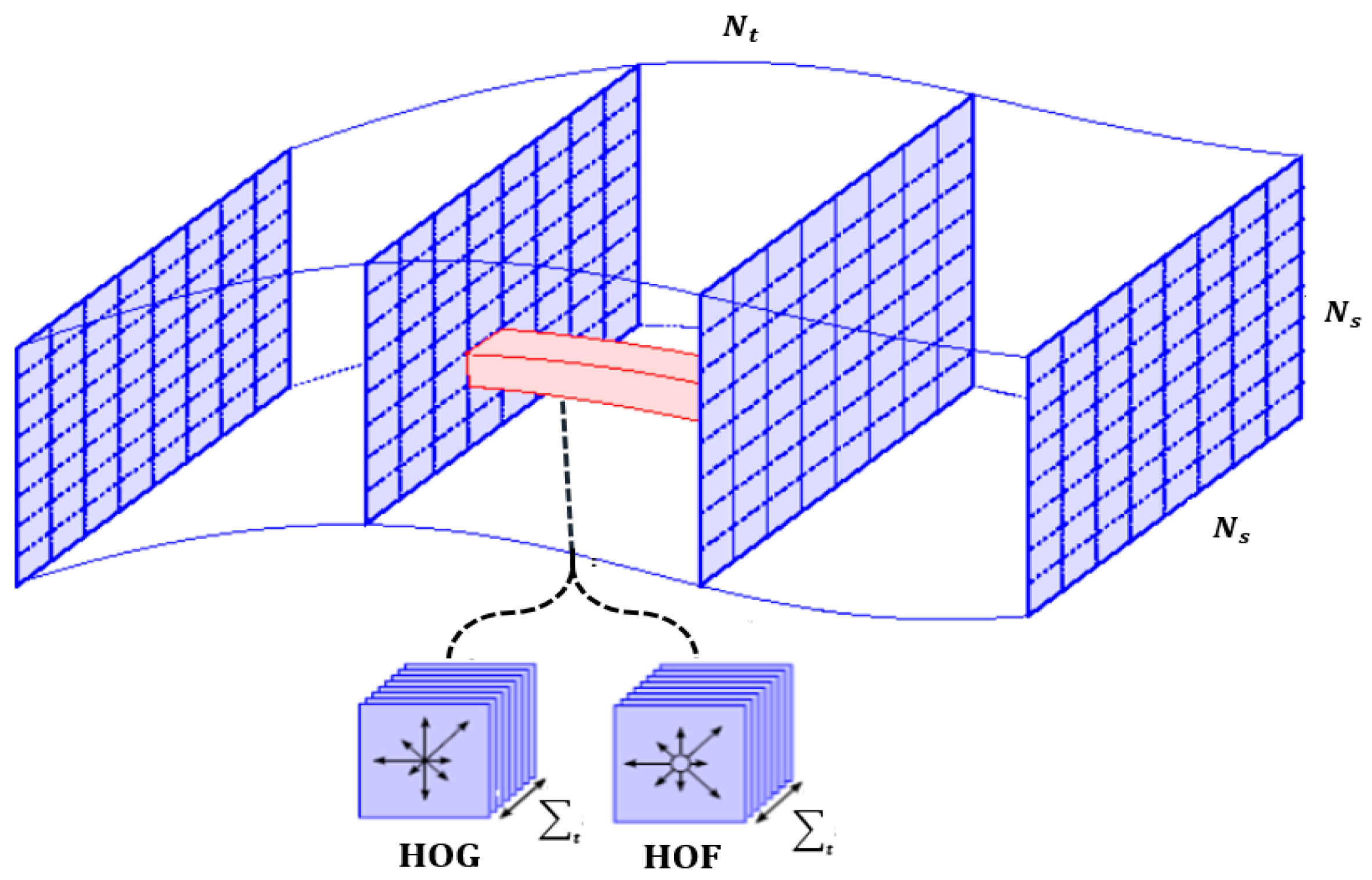
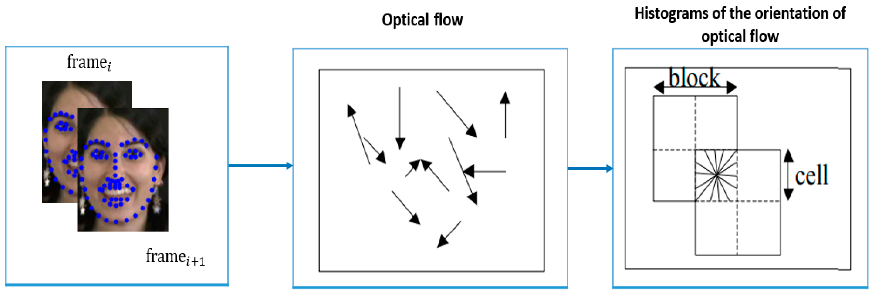
3.2.1. HOF Descriptor
- Optical Flow Computation: Compute the optical flow between consecutive frames of a video sequence. Optical flow represents the motion of objects by analyzing the displacement of pixels between frames.
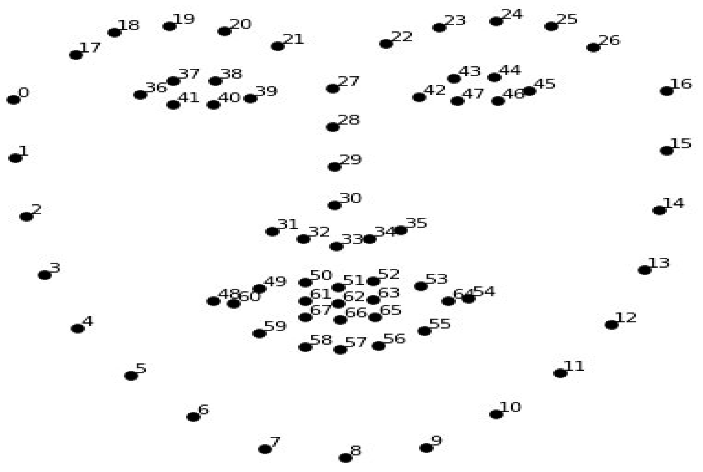
- Dense Grids: Define dense grids over the optical flow field, covering the entire image or region of interest. In our case, we use facial landmarks to track specific points on the face. For example, facial landmarks could include points on the eyes, nose, and mouth.
- Histograms of Orientation: For each grid cell or facial landmark point, calculate histograms of the orientation of optical flow. Divide the optical flow orientations into bins and accumulate the counts of optical flow orientations within each bin.
- Spatial Blocks: Organize the image or region of interest into spatial blocks, where each block contains multiple grid cells or facial landmark points. This step introduces spatial relationships into the descriptor.
- Histograms within Blocks: Compute histograms of optical flow orientations within each spatial block. Similar to the grid cell histograms, quantize orientations into bins and accumulate counts.
- Concatenation: Concatenate the histograms from all spatial blocks merging into just one feature vector. This feature vector represents the overall optical flow-based representation of facial expression dynamics.
- Normalization: Normalize the concatenated feature vector to enhance robustness against variations in lighting and contrast and facial pose.
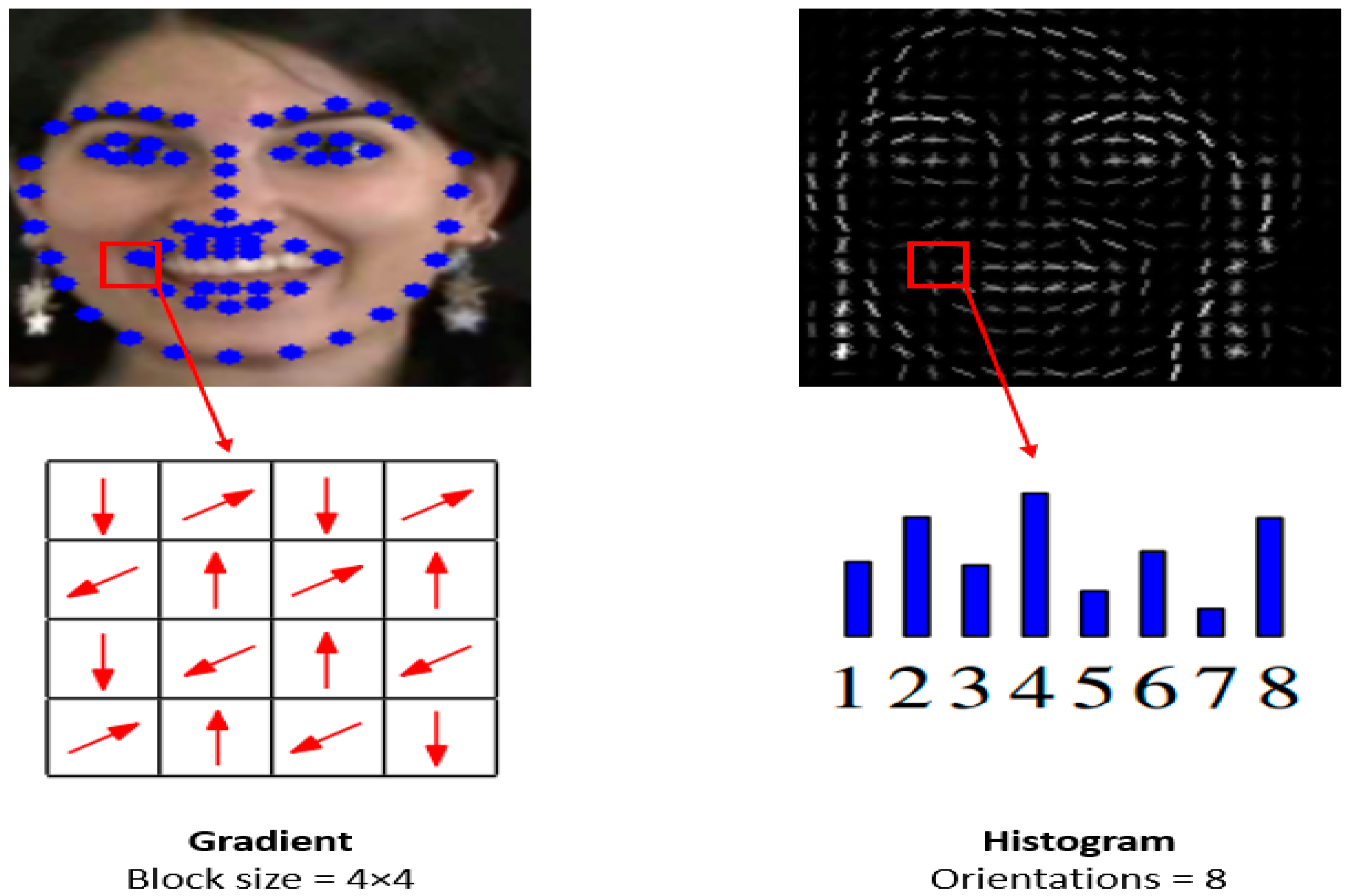
3.2.2. HOG Descriptor
- 1
- Gradient Computation: Compute the image’s gradient to identify edges and intensity changes. This is typically achieved using convolution with specific filters like Sobel filters.
- 2
- Gradient Magnitude and Orientation: Calculate the magnitude () and orientation of the gradient at each pixel (). The magnitude represents the strength of the gradient, while the orientation indicates the direction of the gradient.
- 3.
- Cell Division: Divide the image into cells, which are small regions that will be used to accumulate gradient information. Typically, cells are square and can vary in size.
- 4.
- Histograms within Cells: Create a gradient orientations histogram for each cell. The orientations are quantized into bins, and the histogram captures the distribution of gradient orientations within the cell.
- 5.
- Block Normalization: Organize cells into blocks, which are larger regions consisting of multiple cells. Blocks typically overlap, and within each block, normalize the histograms to account for variations in lighting and contrast.
- 6.
- Concatenation: To create a single feature vector, concatenate each block’s normalized histogram.
- 7.
- Final Normalization: Normalize the concatenated feature vector to ensure robustness to varying illumination and contrast conditions.
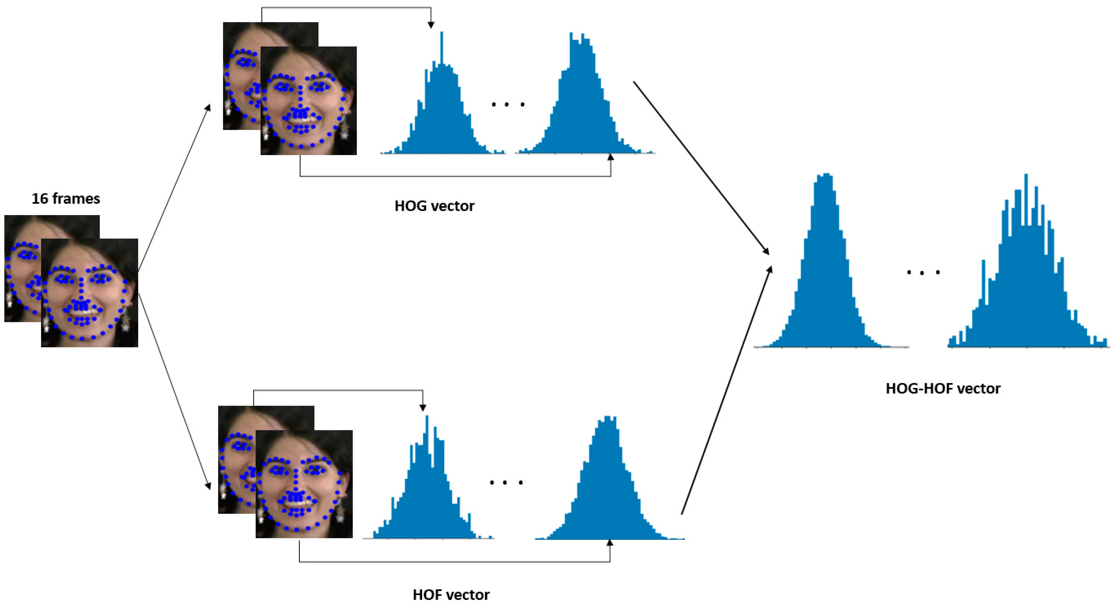
3.2.3. Combination of HOG and HOF
- Video sequence which contains frames with the same height and width .
- Each frame contains numbers of Dlib points, with the height and width .
- Calculate the gradient magnitude and and the orientation at each in the frame.
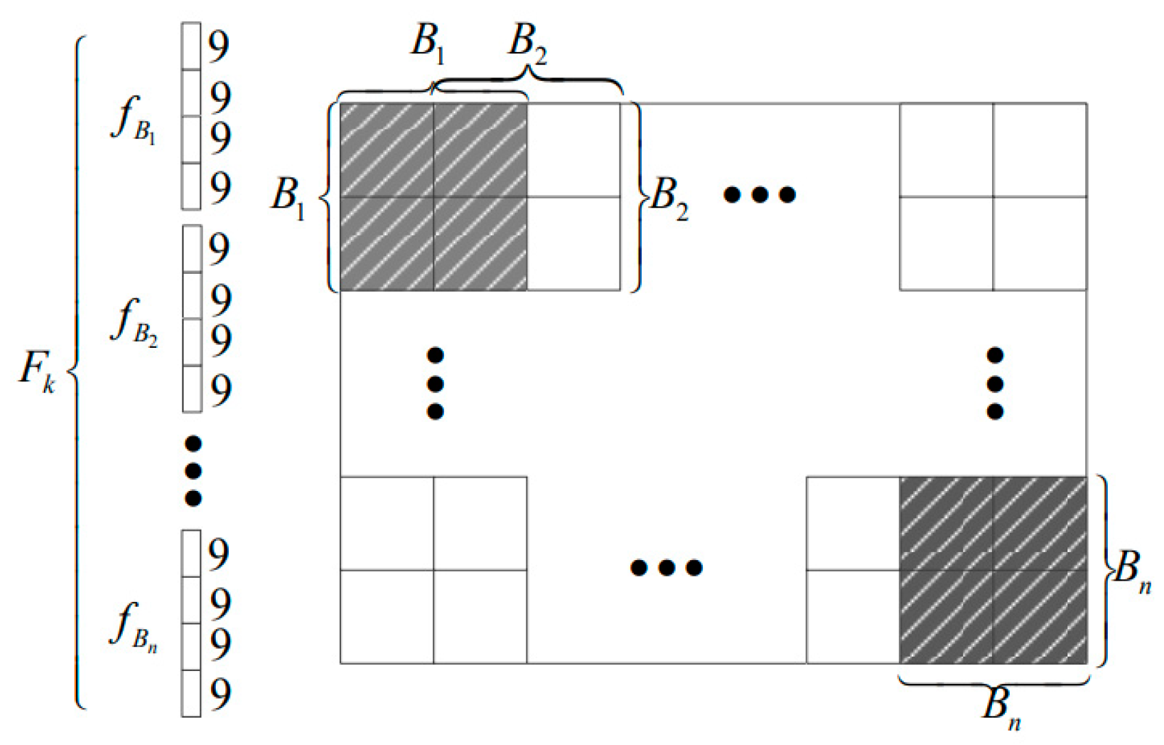
- For each point , create a histogram of gradient orientations vector . Typically, each histogram has nine bins covering 0 to 180 degrees.
- Concatenate all normalized histograms to form the HOG descriptor for the frame: .
- Calculate the optical flow HS between two consecutive frames and in a video sequence.
- For each frame that contains numbers of Dlib points, create a histogram of optical flow directions vector .
- Concatenate all normalized histograms to form the HOF descriptor for the frame: .
- Concatenate the HOG descriptor vector computed for the all frames with the HOF descriptor vector computed from the optical flow between all consecutive frames to create the HOG-HOF vector denoted as :
3.3. Fusion Part
MCB Fusion
- and are the feature matrices from different sources,
- denotes vectorization of a matrix,
- and are projection matrices,
- represents the element-wise product.
- Input features from different modalities: let and be the input feature vectors from two different modalities.
- Randomly project the input feature vectors and into high-dimensional spaces using random projection matrices and . These matrices are randomly generated and are shared across different samples.
- Let and be the projected feature vectors.
- Compute the element-wise (Hadamard) product of the projected feature vectors and :
- Perform Compact Bilinear Pooling (CBP) on the element-wise product .
- CBP is computed by taking the Fast Fourier Transform (FFT) of the element-wise product , followed by operation.
- The resulting compact bilinear pooled feature vector is denoted as .
- The final output of the multimodal compact bilinear pooling operation is the compact bilinear pooled feature vector .
4. Experiment Studies and Result Analysis
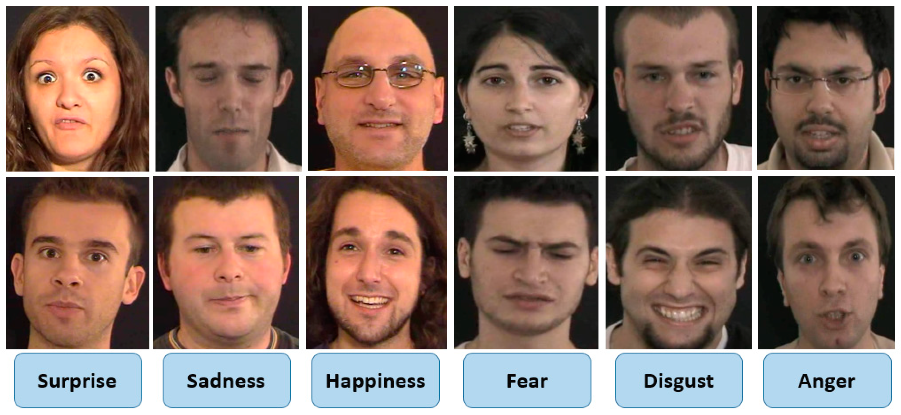
4.1. The Database Selected
4.2. The Classifier Selected
- Feature Vector: Extracted features are transformed into a feature vector, which serves as input to the SVM classifier. This vector represents the unique characteristics of facial expressions in the dataset.
- Training: SVMs are trained using a labeled dataset where each sample is associated with a specific facial expression label. The SVM can identify the optimal hyperplane for separating the various classes.
- Kernel Trick: SVMs frequently convert the input features into a space with more dimensions by using the kernel approach, making it easier to find a hyperplane that separates the classes.
- Cross-Validation: Cross-validation is essential to assess the SVM’s generalization performance. It involves splitting the dataset into training and testing sets multiple times to evaluate the model’s robustness.
- Evaluation Metrics: Common evaluation metrics for facial expression recognition using SVMs include accuracy, precision, recall, and F1 score.
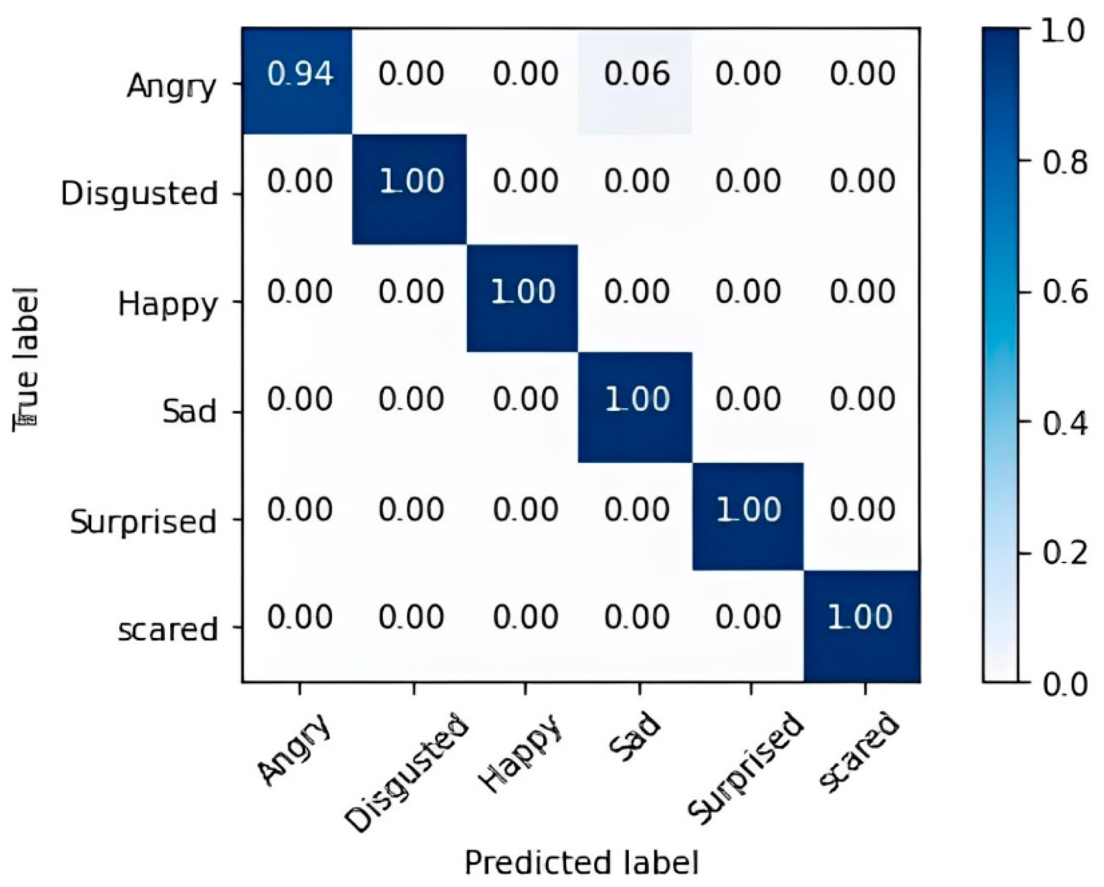
4.3. Experimental Results and Analysis
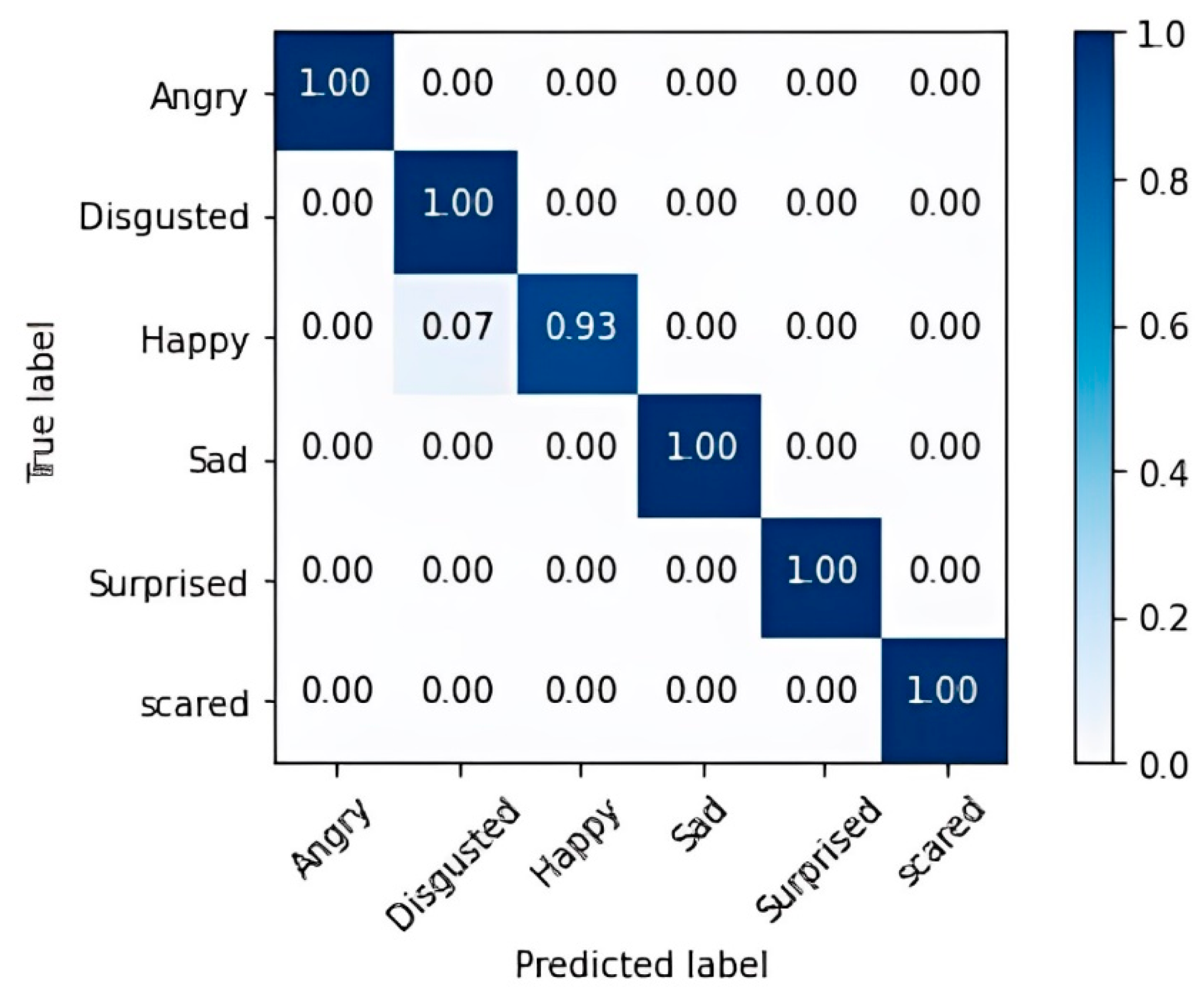
4.3.1. HOG-HOF Method Examination
4.3.2. LSTM Architecture Examination
4.3.3. Methods Vectors Merged
5. Conclusions
Author Contributions
Funding
Data Availability Statement
Acknowledgments
Conflicts of Interest
References
- Efraty, B.; Huang, C.; Shah, S.K.; Kakadiaris, I.A. Facial landmark detection in uncontrolled conditions. In Proceedings of the 2011 International Joint Conference on Biometrics (IJCB), Washington, DC, USA, 11–13 October 2011. [Google Scholar] [CrossRef]
- Ding, J.; Chen, K.; Liu, H.; Huang, L.; Chen, Y.; Lv, Y.; Yang, Q.; Guo, Q.; Han, Z.; Ralph, M.A.L. A unified neurocognitive model of semantics language social behaviour and face recognition in semantic dementia. Nat. Commun. 2020, 11, 1–14. [Google Scholar] [CrossRef]
- Anagnostopoulos, C.N.; Iliou, T.; Giannoukos, I. Features and classifiers for emotion recognition from speech: A survey from 2000 to 2011. Artif. Intell. Rev. 2015, 43, 155–177. [Google Scholar] [CrossRef]
- Dobs, K.; Isik, L.; Pantazis, D.; Kanwisher, N. How face perception unfolds over time. Nat. Commun. 2019, 10, 1–10. [Google Scholar] [CrossRef] [PubMed]
- Kumar, M.P.; Rajagopal, M.K. Detecting facial emotions using normalized minimal feature vectors and semi-supervised twin support vector machines classifier. Appl. Intell. 2019, 49, 4150–4174. [Google Scholar] [CrossRef]
- Kim, Y.; Lee, H.; Provost, E.M. Deep Learning for Robust Feature Generation in Audiovisual Emotion Recognition. In Proceedings of the 2013 IEEE International Conference on Acoustics, Speech and Signal Processing, Vancouver, BC, Canada, 26–31 May 2013; University of Michigan Electrical Engineering and Computer Science: Ann Arbor, MI, USA, 2013; pp. 3687–3691. [Google Scholar]
- Mellouk, W.; Handouzi, W. Facial emotion recognition using deep learning: Review and insights. Procedia Comput. Sci. 2020, 175, 689–694. [Google Scholar] [CrossRef]
- Huang, Y.Y.; Wang, W.Y. Deep residual learning for weakly-supervised relation extraction. In Proceedings of the 2017 Conference on Empirical Methods in Natural Language Processing, Copenhagen, Denmark, 27 September 2017; pp. 1803–1807. [Google Scholar] [CrossRef]
- Simonyan, K.; Zisserman, A. Very deep convolutional networks for large-scale image recognition. In Proceedings of the 3rd International Conference on Learning Representations, ICLR 2015, San Diego, CA, USA, 7–9 May 2015; pp. 1–14. [Google Scholar]
- Staudemeyer, R.C.; Morris, E.R. Understanding LSTM--A tutorial into Long Short-Term Memory Recurrent Neural Networks. arXiv 2019, arXiv:1909.09586, 1–42. [Google Scholar]
- Dalal, N.; Triggs, B. Histograms of Oriented Gradients for Human Detection. In Proceedings of the 2005 IEEE Computer Society Conference on Computer Vision and Pattern Recognition (CVPR’05), San Diego, CA, USA, 20–25 June 2005; pp. 886–893. [Google Scholar]
- Wang, T.; Snoussi, H. Histograms of optical flow orientation for abnormal events detection. In Proceedings of the 2013 IEEE International Workshop on Performance Evaluation of Tracking and Surveillance (PETS), Clearwater Beach, FL, USA, 15–17 January 2013; pp. 45–52. [Google Scholar] [CrossRef]
- Martin, O.; Kotsia, I.; Macq, B.; Pitas, I. The eNTERFACE’05 Audio-Visual emotion database. In Proceedings of the ICDEW 2006—22nd International Conference on Data Engineering Workshops (ICDEW’06), Atlanta, GA, USA, 3–7 April 2006; pp. 2–9. [Google Scholar] [CrossRef]
- Liu, P.; Han, S.; Meng, Z.; Tong, Y. Facial expression recognition via a boosted deep belief network. In Proceedings of the 2014 IEEE Conference on Computer Vision and Pattern Recognition, Columbus, OH, USA, 23–28 June 2014; pp. 1805–1812. [Google Scholar] [CrossRef]
- Mollahosseini, A.; Chan, D.; Mahoor, M.H. Going deeper in facial expression recognition using deep neural networks. In Proceedings of the 2016 IEEE Winter Conference on Applications of Computer Vision (WACV), Lake Placid, NY, USA, 7–10 March 2016. [Google Scholar] [CrossRef]
- Zhang, F.; Zhang, T.; Mao, Q.; Xu, C. Joint Pose and Expression Modeling for Facial Expression Recognition. In Proceedings of the 2018 IEEE/CVF Conference on Computer Vision and Pattern Recognition, Salt Lake City, UT, USA, 18–23 June 2018; pp. 3359–3368. [Google Scholar] [CrossRef]
- Zhao, X.; Liang, X.; Liu, L.; Li, T.; Han, Y.; Vasconcelos, N.; Yan, S. Peak-piloted deep network for facial expression recognition. In Computer Vision–ECCV 2016, Lecture Notes in Computer Science (Including Subser. Lect. Notes Artif. Intell. Lect. Notes Bioinformatics); Springer: Cham, Switzerland, 2016; Volume 9906, pp. 425–442. [Google Scholar] [CrossRef]
- Lowe, D.G. Distinctive image features from scale-invariant keypoints. Int. J. Comput. Vis. 2004, 60, 91–110. [Google Scholar] [CrossRef]
- Scovanner, P.; Ali, S.; Shah, M. A 3-dimensional sift descriptor and its application to action recognition. In Proceedings of the 15th ACM International Conference on Multimedia, Augsburg Germany, 25–29 September 2007; pp. 357–360. [Google Scholar] [CrossRef]
- Kläser, A.; Marszałek, M.; Schmid, C. A spatio-temporal descriptor based on 3D-gradients. In Proceedings of the BMVC 2008—British Machine Vision Conference 2008, Leeds, UK, 1 September 2008. [Google Scholar] [CrossRef]
- Dalal, N.; Triggs, B.; Schmid, C. Human Detection Using Oriented Histograms of Flow and Appearance to cite this version: Human Detection using Oriented Histograms of Flow and Appearance. In Computer Vision–ECCV 2006, Lecture Notes in Computer Science, European Conference on Computer Vision; LNIP; Springer: Berlin/Heidelberg, Germany, 2006; Volume 3952, pp. 428–441. [Google Scholar]
- Laptev, I.; Marszałek, M.; Schmid, C.; Rozenfeld, B. Learning realistic human actions from movies. In Proceedings of the 2008 IEEE Conference on Computer Vision and Pattern Recognition, CVPR, Anchorage, AK, USA, 23–28 June 2008; pp. 1–7. [Google Scholar] [CrossRef]
- Corneanu, C.A.; Simón, M.O.; Cohn, J.F.; Guerrero, S.E. Survey on RGB, 3D, Thermal, and Multimodal Approaches for Facial Expression Recognition: History, Trends, and Affect-Related Applications. IEEE Trans. Pattern Anal. Mach. Intell. 2016, 38, 1548–1568. [Google Scholar] [CrossRef]
- Li, R.; Tian, J.; Chua, M.C.H. Facial expression classification using salient pattern driven integrated geometric and textual features. Multimed. Tools Appl. 2019, 78, 28971–28983. [Google Scholar] [CrossRef]
- Sadeghi, H.; Raie, A.A. Human vision inspired feature extraction for facial expression recognition. Multimed. Tools Appl. 2019, 78, 30335–30353. [Google Scholar] [CrossRef]
- Sharma, M.; Jalal, A.S.; Khan, A. Emotion recognition using facial expression by fusing key points descriptor and texture features. Multimed. Tools Appl. 2019, 78, 16195–16219. [Google Scholar] [CrossRef]
- Lakshmi, D.; Ponnusamy, R. Facial emotion recognition using modified HOG and LBP features with deep stacked autoencoders. Microprocess. Microsyst. 2021, 82, 103834. [Google Scholar] [CrossRef]
- Cai, J.; Chang, O.; Tang, X.L.; Xue, C.; Wei, C. Facial Expression Recognition Method Based on Sparse Batch Normalization CNN. In Proceedings of the 2018 37th Chinese Control Conference (CCC), Wuhan, China, 25–27 July 2018; pp. 9608–9613. [Google Scholar] [CrossRef]
- Agrawal, A.; Mittal, N. Using CNN for facial expression recognition: A study of the effects of kernel size and number of filters on accuracy. Vis. Comput. 2020, 36, 405–412. [Google Scholar] [CrossRef]
- Li, Y.; Zeng, J.; Shan, S.; Chen, X. Occlusion Aware Facial Expression Recognition Using CNN with Attention Mechanism. IEEE Trans. Image Process. 2019, 28, 2439–2450. [Google Scholar] [CrossRef]
- Kim, D.H.; Baddar, W.J.; Jang, J.; Ro, Y.M. Multi-objective based spatio-temporal feature representation learning robust to expression intensity variations for facial expression recognition. IEEE Trans. Affect. Comput. 2019, 10, 223–236. [Google Scholar] [CrossRef]
- Yolcu, G.; Oztel, I.; Kazan, S.; Oz, C.; Palaniappan, K.; Lever, T.E.; Bunyak, F. Facial expression recognition for monitoring neurological disorders based on convolutional neural network. Multimed. Tools Appl. 2019, 78, 31581–31603. [Google Scholar] [CrossRef]
- Chouhayebi, H.; Mahraz, M.A.; Riffi, J.; Tairi, H. A dynamic fusion of features from deep learning and the HOG-TOP algorithm for facial expression recognition. Multimed. Tools Appl. 2023 83, 32993–33017. [CrossRef]
- Hu, Z.; Wang, L.; Luo, Y.; Xia, Y.; Xiao, H. Speech Emotion Recognition Model Based on Attention CNN Bi-GRU Fusing Visual Information. Eng. Lett. 2022, 30, 427–434. [Google Scholar]
- Priyasad, D.; Fernando, T.; Denman, S.; Sridharan, S.; Fookes, C. Attention Driven Fusion for Multi-Modal Emotion Recognition. In Proceedings of the ICASSP 2020—2020 IEEE International Conference on Acoustics, Speech and Signal Processing (ICASSP), Barcelona, Spain, 4–8 May 2020; pp. 3227–3231. [Google Scholar] [CrossRef]
- Chowdary, M.K.; Nguyen, T.N.; Hemanth, D.J. Deep learning-based facial emotion recognition for human–computer interaction applications. Neural Comput. Appl. 2023, 35, 23311–23328. [Google Scholar] [CrossRef]
- Li, B. Facial expression recognition via transfer learning. EAI Endorsed Trans. e-Learn. 2021, 169180. [Google Scholar] [CrossRef]
- Priyasad, D.; Fernando, T.; Denman, S.; Sridharan, S.; Fookes, C. Learning Salient Features for Multimodal Emotion Recognition with Recurrent Neural Networks and Attention Based Fusion. In Proceedings of the 15th International Conference on Auditory-Visual Speech Processing, Melbourne, Australia, 10–11 August 2019; pp. 21–26. [Google Scholar] [CrossRef]
- Deng, J.; Dong, W.; Socher, R.; Li, L.-J.; Li, K.; Fei-Fei, L. ImageNet: A large-scale hierarchical image database. In Proceedings of the 2009 IEEE Conference on Computer Vision and Pattern Recognition, Miami, FL, USA, 20–25 June 2010; pp. 248–255. [Google Scholar] [CrossRef]
- Konečný, J.; Hagara, M. One-shot-learning gesture recognition using HOG-HOF features. J. Mach. Learn. Res. 2014, 15, 2513–2532. [Google Scholar] [CrossRef]
- Harris, C.; Stephens, M. A Combined Corner and Edge Detector. In Proceedings of the Alvey Vision Conference, AVC 1988, Manchester, UK, 1 September 1988; pp. 23.1–23.6. [Google Scholar] [CrossRef]
- Wang, H.; Ullah, M.M.; Kläser, A.; Laptev, I.; Schmid, C. Evaluation of local spatio-temporal features for action recognition. In Proceedings of the British Machine Vision Conference, BMVC 2009, London, UK, 7–10 September 2009. [Google Scholar] [CrossRef]
- Wang, H.; Kläser, A.; Schmid, C.; Liu, C.L. Dense trajectories and motion boundary descriptors for action recognition. Int. J. Comput. Vis. 2013, 103, 60–79. [Google Scholar] [CrossRef]
- King, D.E. Dlib-ml: A machine learning toolkit. J. Mach. Learn. Res. 2009, 10, 1755–1758. [Google Scholar]
- Horn, B.K.P.; Schunck, B.G. Determining optical flow. Artif. Intell. 1981, 17, 185–203. [Google Scholar] [CrossRef]
- Sun, D.; Roth, S.; Black, M.J. Secrets of optical flow estimation and their principles. In Proceedings of the 2010 IEEE Computer Society Conference on Computer Vision and Pattern Recognition, San Francisco, CA, USA, 13–18 June 2010; pp. 2432–2439. [Google Scholar] [CrossRef]
- Farneb, G. Two-Frame Motion Estimation Based on polynomial expansion. Lect. Notes Comput. Sci. 2003, 2749, 363–370. [Google Scholar]
- Dalal, N.; People, F.; Interaction, V.H. Finding People in Images and Videos. Ph.D. Thesis, Institut National Polytechnique de Grenoble–INPG, Grenoble, France, 2006; p. 150. [Google Scholar]
- Fukui, A.; Park, D.H.; Yang, D.; Rohrbach, A.; Darrell, T.; Rohrbach, M. Multimodal compact bilinear pooling for visual question answering and visual grounding. In Proceedings of the EMNLP 2016—2016 Conference on Empirical Methods in Natural Language Processing, Austin, TX, USA, 1–4 November 2016; pp. 457–468. [Google Scholar] [CrossRef]
- eNTERFACE05. Available online: www.enterface.net/enterface05/docs/results/databases/project1_database.zip (accessed on 6 March 2024).


| Emotion | Precision | Recall | F1-Score |
|---|---|---|---|
| Angry | 100.00 | 100.00 | 100.00 |
| Disgusted | 100.00 | 100.00 | 100.00 |
| Happy | 100.00 | 100.00 | 100.00 |
| Sad | 100.00 | 100.00 | 100.00 |
| Surprised | 100.00 | 92.30 | 96.00 |
| Scared | 85.71 | 100.00 | 92.30 |
| Accuracy | - | - | 98.03 |
| Macro avg | 97.61 | 98.71 | 98.05 |
| Weighted avg | 98.31 | 98.03 | 98.07 |
| Model Hyperparameter Name | Value |
|---|---|
| LSTM layer 1 | 500 |
| LSTM layer 2 | 350 |
| LSTM layer 3 | 250 |
| Dense layer | 256 |
| Activation Function | Relu |
| Dense layer | 4096 |
| Activation Function | Relu |
| Epochs | 2000 |
| Optimizer | adam |
| DropOut ratio | 0.2 |
| Emotion | Precision | Recall | F1-Score |
|---|---|---|---|
| Angry | 100.00 | 94.11 | 96.97 |
| Disgusted | 100.00 | 100.00 | 100.00 |
| Happy | 100.00 | 100.00 | 100.00 |
| Sad | 93.33 | 100.00 | 96.55 |
| Surprised | 100.00 | 100.00 | 100.00 |
| Scared | 100.00 | 100.00 | 100.00 |
| Accuracy | - | - | 98.30 |
| Macro avg | 98.88 | 99.02 | 98.92 |
| Weighted avg | 98.41 | 98.30 | 98.30 |
| Emotion | Precision | Recall | F1-Score |
|---|---|---|---|
| Angry | 100.00 | 100.00 | 100.00 |
| Disgusted | 87.50 | 100.00 | 93.33 |
| Happy | 100.00 | 92.85 | 96.29 |
| Sad | 100.00 | 100.00 | 100.00 |
| Scared | 100.00 | 100.00 | 100.00 |
| Surprised | 100.00 | 100.00 | 100.00 |
| Accuracy | - | - | 98.24 |
| Macro avg | 97.91 | 98.81 | 98.27 |
| Weighted avg | 98.46 | 98.24 | 98.27 |
| Emotion | Precision | Recall | F1-Score |
|---|---|---|---|
| Angry | 85.71 | 100.00 | 92.30 |
| Disgusted | 100.00 | 100.00 | 100.00 |
| Happy | 100.00 | 83.33 | 90.90 |
| Sad | 100.00 | 100.00 | 100.00 |
| Scared | 100.00 | 100.00 | 100.00 |
| Surprised | 100.00 | 100.00 | 100.00 |
| Accuracy | - | - | 97.14 |
| Macro avg | 97.61 | 97.22 | 97.20 |
| Weighted avg | 97.55 | 97.14 | 97.12 |
| Method | Accuracy |
|---|---|
| Chouhayebi et al. [33] | 96.89% |
| Hu et al. [34] | 89.65% |
| Priyasad et al. [35] | 80.51% |
| Priyasad et al. [38] | 97.75% |
| Proposed method | 98.24% |
| Method | Accuracy |
|---|---|
| ResNet VGG19 LSTM | 98.30% |
| HOG-HOF | 98.03% |
| Fusion with basic concatenation | 98.24% |
| Fusion with MCB algorithm | 97.14% |
Disclaimer/Publisher’s Note: The statements, opinions and data contained in all publications are solely those of the individual author(s) and contributor(s) and not of MDPI and/or the editor(s). MDPI and/or the editor(s) disclaim responsibility for any injury to people or property resulting from any ideas, methods, instructions or products referred to in the content. |
© 2024 by the authors. Licensee MDPI, Basel, Switzerland. This article is an open access article distributed under the terms and conditions of the Creative Commons Attribution (CC BY) license (https://creativecommons.org/licenses/by/4.0/).
Share and Cite
Chouhayebi, H.; Mahraz, M.A.; Riffi, J.; Tairi, H.; Alioua, N. Human Emotion Recognition Based on Spatio-Temporal Facial Features Using HOG-HOF and VGG-LSTM. Computers 2024, 13, 101. https://doi.org/10.3390/computers13040101
Chouhayebi H, Mahraz MA, Riffi J, Tairi H, Alioua N. Human Emotion Recognition Based on Spatio-Temporal Facial Features Using HOG-HOF and VGG-LSTM. Computers. 2024; 13(4):101. https://doi.org/10.3390/computers13040101
Chicago/Turabian StyleChouhayebi, Hajar, Mohamed Adnane Mahraz, Jamal Riffi, Hamid Tairi, and Nawal Alioua. 2024. "Human Emotion Recognition Based on Spatio-Temporal Facial Features Using HOG-HOF and VGG-LSTM" Computers 13, no. 4: 101. https://doi.org/10.3390/computers13040101
APA StyleChouhayebi, H., Mahraz, M. A., Riffi, J., Tairi, H., & Alioua, N. (2024). Human Emotion Recognition Based on Spatio-Temporal Facial Features Using HOG-HOF and VGG-LSTM. Computers, 13(4), 101. https://doi.org/10.3390/computers13040101