Rational Play in Extensive-Form Games

Abstract

We argue in favor of a departure from the equilibrium approach in game theory towards the less ambitious goal of describing only the actual behavior of rational players. The notions of Nash equilibrium and its refinements require a specification of the players’ choices and beliefs not only along the equilibrium play but also at counterfactual histories. We discuss an alternative—counterfactual-free—approach that focuses on choices and beliefs along the actual play, while being silent on choices and beliefs at unreached histories. Such an approach was introduced in an earlier paper that considered only perfect-information games. Here we extend the analysis to general extensive-form games (allowing for imperfect information) and put forward a behavioral notion of self-confirming play, which is close in spirit to the literature on self-confirming equilibrium. We also extend, to general extensive-form games, the characterization of rational play that is compatible with pure-strategy Nash equilibrium.

1. Introduction

We address the issue of what kind of object qualifies as a “rational solution” of an extensive-form game. Whereas the dominant approach focuses on strategy profiles that, besides being Nash equilibria, satisfy additional—often increasingly complex—criteria, we suggest moving in the opposite direction by doing without the notion of strategy and focusing only on the actions and beliefs of the active players, that is, on choices made and beliefs held at reached histories.

The notions of Nash equilibrium and its refinements require a specification of the players’ choices and beliefs not only along the equilibrium play but also at counterfactual (that is, unreached) histories. In Section 2, we argue that pinning down counterfactual choices at unreached information histories is not a straightforward matter and that it may be futile to search for a general theory of rationality that can achieve this result. Instead, we argue in favor of a more basic approach that was put forward in [1]; while [1] was exclusively focused on perfect-information games, in this paper we extend the approach to general extensive-form games, by allowing for imperfect information. We put forward a behavior-based notion of self-confirming play—which is close in spirit to the literature on self-confirming equilibrium—and extend the characterization of rational play that is compatible with pure-strategy Nash equilibrium to general extensive-form games.

The paper is organized as follows. In Section 2, we illustrate, by means of examples, the difficulties that arise in the pursuit of specifying rational choices and beliefs at unreached information sets. In Section 3, we review the behavioral models introduced in [1], extend them to general extensive-form games and put forward a notion of self-confirming play, where each action taken is justified by the beliefs held at the time of choice and, furthermore, those beliefs turn out to be exactly correct, so that no player receives information that contradicts those beliefs (and thus experiences no regret). We also extend the characterization of rational play that is consistent with pure-strategy Nash equilibrium to general extensive-form games. Section 4 provides further discussion and a conclusion.

2. What Is a Rational Solution?

What constitutes a rational solution of an extensive-form game? Two different approaches can be found in the literature.

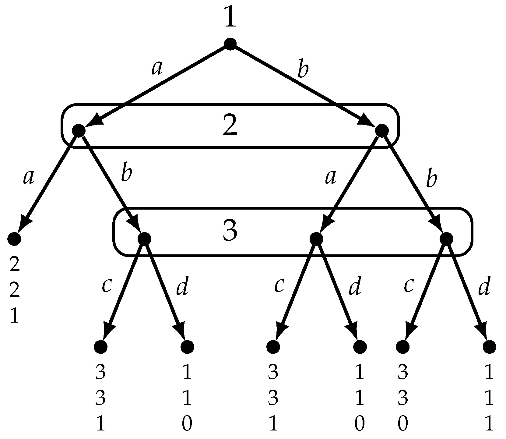
1. The Nash-equilibrium approach. Within this approach the notion of rationality is captured through the concept of Nash equilibrium or one of its refinements. Consider, for example, the game of Figure 1 and the strategy profile $(a,a,d)$.

Although $(a,a,d)$ is a Nash equilibrium, popular refinements of Nash equilibrium would deny it the status of a “rational solution” [for example, $(a,a,d)$ is not a sequential equilibrium [2] because strategy d can be a rational choice for Player 3 only if she assigns positive probability to history $bb$, but the notion of consistency— which is part of the definition of sequential equilibrium—requires Player 3’s beliefs to assign zero probability to $bb$]. Regardless of one’s views on whether $(a,a,d)$ can be considered a rational solution of the game of Figure 1, there is a more fundamental issue to be considered, namely how Player 3’s strategy d should be interpreted. The common interpretation seems to be in terms of an objective counterfactual: Player 3 would play d if her information set were to be reached. It is typically the case in extensive-form games that, given a strategy profile s, there will be information sets that are not reached by the play generated by s. Thus, under this interpretation of strategies, a rational solution of the game would determine, not only what actions are actually taken by the players (that is, what the actual play of the game is), but also—counterfactually— what actions would be taken at every unreached information set.

The standard theory of counterfactuals, due to Robert Stalnaker and David Lewis [3,4,5], postulates a family of similarity relations on the set of possible worlds (one for each possible world) and the sentence “if $\varphi$ were the case then $\psi$ would be the case” is declared to be true at a possible world $\omega$ if $\psi$ is true at the most similar world(s) to $\omega$ where $\varphi$ is true. Referring to the game of Figure 1, at a world where Players 1 and 2 play $aa$, we can take $\varphi$ to be the sentence “Player 3’s information set is reached” and $\psi$ the sentence “Player 3 plays d”. Then the sentence “if $\varphi$ were the case then $\psi$ would be the case” would be true at the actual world (where Player 3’s information set is not reached, because Players 1 and 2 play $aa$) if and only if the most similar world to the actual world at which Player 3’s information is reached is one where Player 3 plays d. However, how are we to determine if the most similar world to the actual world is one where Player 3 plays d or one where Player 3 plays c?

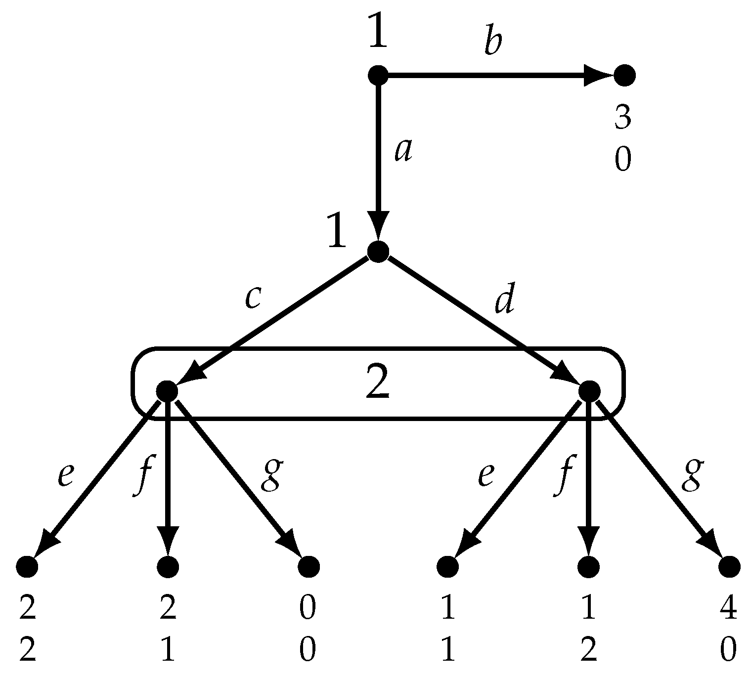
In general, pinning down counterfactual choices at unreached information sets is not a straightforward matter. Consider, for example, the game illustrated in Figure 2 due to Perea ([6], p. 169), where Player 1 can either play b and end the game, or play a, in which case Players 1 and 2 play a “simultaneous” game.

If one appeals to backward-induction reasoning, one is led to conclude that the “rational solution” of this game is the strategy profile $(b,e)$, which incorporates the counterfactual claim that Player 2 would play e if her information set were to be reached [first apply the procedure of iterative deletion of strictly dominated strategies to the subgame that starts at history a to obtain $(c,e)$: in the subgame, for Player 2 g is strictly dominated by both e and f; after deleting g, for Player 1 d becomes strictly dominated by c; after deleting d, for Player 2 f becomes strictly dominated by e; then infer that Player 1 will play b; backward-induction reasoning is captured by such notions as “common belief in present and future rationality” [7], or forward belief in rationality [8,9].]

On the other hand, if one appeals to forward-induction reasoning (as captured by the notion of extensive-form rationalizability [10,11]) one is led to conclude that the “rational solution” of this game is the strategy profile $(b,f)$, incorporating the counterfactual claim that Player 2 would play f if her information set were to be reached [first eliminate Player 1’s strategy $ac$, since it is strictly dominated by b, and Player 2’s strategy g; then eliminate Player 1’s strategy $ad$ and Player 2’s strategy e, with the conclusion that Player 1 will play b and Player 2 would play f.]

Note, however, that the prediction in terms of play is the same, namely that Player 1 would end the game by playing b; the two solutions differ only in terms of the answer to the question “what would Player 2 do if her information set were to be reached?”

The above example shows that it may be futile to search for a general theory of rationality that would pin down counterfactual choices and beliefs at unreached information sets (as shown recently by [12], besides backward-induction and forward-induction reasoning, there are other types of rationality-based reasoning that lead to the same outcome but different counterfactual “predictions” about choices at unreached information sets). It is natural, therefore, to ask: Is it essential to provide an answer to such counterfactual questions? The thesis put forward in this paper is that the answer to this question is negative.

2. The self-confirming equilibrium approach. Returning to the strategy profile $(a,a,d)$ in the game of Figure 1, an alternative approach is to interpret Player 3’s strategy d not as a claim about what Player 3 would actually do in a counterfactual world where her information is reached, but as a belief, shared by Players 1 and 2, about Player 3’s hypothetical behavior. Such shared belief would support the rationality of playing a for both Players 1 and 2.

This approach is in line with the literature that identifies rational play in extensive-form games with the notion of self-confirming equilibrium, introduced in [13] (similar notions are put forward in [14,15,16]; Refs. [17,18] provide a refinement of self-confirming equilibrium that imposes constraints on the players’ beliefs about what actions an opponent could take at an off-path information set and [19] provide a generalization of self-confirming equilibrium; the related expression ‘conjectural equilibrium’ is mostly used in the context of strategic-form games: it was introduced in this context by [20,21] and is defined as a situation where each player’s strategy is a best response to a conjecture about the other players’ strategies and any information acquired after the play of the game does not induce the player to change her conjecture). A self-confirming equilibrium is a strategy profile satisfying the property that each player’s strategy is a best response to her beliefs about the strategies of her opponents, and each player’s beliefs are correct along the equilibrium play, even though beliefs about play at unreached information sets may be incorrect. The essential feature of a self-confirming equilibrium is that no player receives information that contradicts her beliefs.

If one follows the interpretation suggested above, then two issues arise. First of all, the strategy profile $(a,a,d)$ (for the game of Figure 1) is now a hybrid object, incorporating—on the one hand—a prediction about actual behavior (namely, the $(a,a)$ part) and—on the other hand – an encoding of the beliefs of Players 1 and 2 (namely, the d part). This leaves to be desired, since one should clearly distinguish between actions and beliefs and model the latter explicitly. The second issue is that there seems to be no reason to require different players to agree on the hypothetical choice of a third player at an unreached information set. Consider, for example, the game of Figure 3, taken from ([13], p. 533).

In this game it is rational for Player 1 to play a, if she believes that Player 2 will play A and Player 3 would play L, and it is rational for Player 2 to play A, if he believes that Player 3 would play R. Thus, the play $aA$ is supported by beliefs of Players 1 and 2 that are not in agreement with each other.

Note, however, that the notion of self-confirming equilibrium is still defined in terms of a strategy profile and thus one cannot claim that $(a,A)$ is a self-confirming equilibrium. One would have to state that both $(a,A,L)$ and $(a,A,R)$ are self-confirming equilibria sustained by Player 1’s belief (correct in the former, erroneous in the latter) that Player 3 would play L and Player 2’s belief (erroneous in the former, correct in the latter) that Player 3 would play R. In other words, also the notion of self-confirming equilibrium requires an answer to the counterfactual “what would Player 3 do if her information set were to be reached?” Note also that in the game of Figure 3 there is no Nash equilibrium that yields the play $aA$; thus, a self-confirming equilibrium need not be a Nash equilibrium.

Both the notion of Nash equilibrium and the notion of self-confirming equilibrium require specifying choices at all information sets, whether they are reached or not. From a conceptual point of view, however, it is not clear what role choices at unreached information sets play beyond expressing the beliefs of the active players along the equilibrium path. For example, consider again the game of Figure 3 and a situation where Player 1 plays a – believing that Player 2 will play A and Player 3 would play L–and Player 2 plays A, believing that Player 3 would play R. Why is this not enough as a “solution”? Why the need to settle the counterfactual concerning what Player 3 would truly do if her information set were to be reached and thus which of Players 1 and 2 is holding incorrect beliefs? [Note that, as [15] points out, in this game Player 3 gains from the uncertainty in the minds of Players 1 and 2 and, if asked what she would do, she would refuse to answer, since her payoff is largest when Players 1 and 2 play $aA$.] Furthermore, it is not clear how the counterfactual could be settled: both L and R can be justified as hypothetical rational choices for Player 3.

In this paper, we turn to an alternative approach, put forward in [1] in the context of perfect-information games, and extend it to general extensive-from games. The proposed framework restricts attention to the actual choices of the players and the beliefs that justify those choices.

3. Behavioral Models of Games

There are two types of epistemic/doxastic models used in the game-theoretic literature: the so-called “state-space” models and the “type-space” models. We will adopt the former (note that there is a straightforward way of translating one type of model into the other). In the standard state-space model of a given game, one takes as starting point a set of states (or possible worlds) and associates with every state a strategy for every player, thus providing an interpretation of a state in terms of players’ choices. If $\omega$ is a state and $s_i$ is the strategy of player i at $\omega$ then the interpretation is that, at that state, player i plays $s_i$. If the game is simultaneous (so that there cannot be any unreached information sets), then there is no ambiguity in the expression “player i plays $s_i$”, but if the game is an extensive-form game then the expression is ambiguous. Consider, for example, the game of Figure 1 and a state $\omega$ where Players 1 and 2 play $aa$, so that Player 3’s information set is not reached; suppose also that the strategy of Player 3 associated with state $\omega$ is d. In what sense does Player 3 “play” d? Does it mean that, before the game starts, Player 3 has made a plan to play d if her information happens to be reached? Or does it mean (in a Stalnaker-Lewis interpretation of the counterfactual) that in the state most similar to $\omega$ where her information set is actually reached, Player 3 plays d? [This interpretation is adopted in [22] where it is pointed out that in this type of models “one possible culprit for the confusion in the literature regarding what is required to force the backward induction solution in games of perfect information is the notion of a strategy”.] Or is Player 3’s strategy d to be interpreted not as a statement about what Player 3 would do but as an expression of what the opponents think that Player 3 would do?

While most of the literature on the epistemic foundations of game theory makes use of strategy-based models, a few papers follow a behavioral approach by associating with each state a play (or outcome) of the game (the seminal contribution is [23], followed by [1,8,24,25]; the focus of this literature has been on games with perfect information). The challenge in this class of models is to capture the reasoning of a player who takes a particular action while considering what would happen if she took a different action. The most common approach is to postulate, for each player, a set of conditional beliefs, where the conditioning events are represented by possible histories in the game, including off-path histories ([23] uses extended information structures to model hypothetical knowledge, [8] use plausibility relations and [24] use conditional probability systems). Here we follow the simpler approach put forward in [1], which models the “pre-choice” beliefs of a player, while the previous literature considered the “after-choice” beliefs. The previous literature was based on the assumption that, if at a state a player takes action a, then she knows that she takes action a, that is, in all the states that she considers possible she takes action a. The pre-choice or deliberation stage approach, on the other hand, models the beliefs of the player at the time when she is contemplating the actions available to her and treats each of those actions as an “open possibility”. Thus, her beliefs take the following form: “if I take action a then the outcome will be x and if I take action b then the outcome will be y”, where the conditional “if p then q” is interpreted as a material conditional, that is, as equivalent to “either not p or q” (in [26] it is argued that, contrary to a common view, the material conditional is indeed sufficient to model deliberation; it is also shown how to convert pre-choice beliefs into after-choice beliefs, reflecting a later stage at which the agent has made up her mind on what to do). This analysis does not rely in any way on counterfactuals; furthermore, only the beliefs of the active players at the time of choice are modeled, so that no initial beliefs nor belief revision policies are postulated. The approach is described below and it makes use of the history-based definition of extensive-form game, which is reviewed in Appendix A.

As in [1] we take a non-quantitative approach based on qualitative beliefs and ordinal utility.

3.1. Qualitative Beliefs

Let $\mathrm{\Omega }$ be a set, whose elements are called states (or possible worlds). We represent the beliefs of an agent by means of a binary relation $\mathcal{B}\subseteq \mathrm{\Omega }\times \mathrm{\Omega }$. The interpretation of $(\omega ,{\omega }^{\prime })\in \mathcal{B}$, also denoted by $\omega \mathcal{B}{\omega }^{\prime }$, is that at state $\omega$ the agent considers state ${\omega }^{\prime }$ possible; we also say that ${\omega }^{\prime }$ is reachable from $\omega$ by $\mathcal{B}$. For every $\omega \in \mathrm{\Omega }$ we denote by $\mathcal{B}\left(\omega \right)$ the set of states that are reachable from $\omega$, that is, $\mathcal{B}\left(\omega \right)=\{{\omega }^{\prime }\in \mathrm{\Omega }:\omega \mathcal{B}{\omega }^{\prime }\}$.

$\mathcal{B}$ is transitive if ${\omega }^{\prime }\in \mathcal{B}\left(\omega \right)$ implies $\mathcal{B}\left({\omega }^{\prime }\right)\subseteq \mathcal{B}\left(\omega \right)$ and it is euclidean if ${\omega }^{\prime }\in \mathcal{B}\left(\omega \right)$ implies $\mathcal{B}\left(\omega \right)\subseteq \mathcal{B}\left({\omega }^{\prime }\right)$ (it is well known that transitivity of $\mathcal{B}$ corresponds to positive introspection of beliefs: if the agent believes an event $\mathbf{E}$ then she believes that she believes $\mathbf{E}$, and euclideanness corresponds to negative introspection: if the agent does not believe $\mathbf{E}$ then she believes that she does not believe $\mathbf{E}$). We will assume throughout that the belief relations are transitive and euclidean so that ${\omega }^{\prime }\in \mathcal{B}\left(\omega \right)$ implies that $\mathcal{B}\left({\omega }^{\prime }\right)=\mathcal{B}\left(\omega \right)$. Note that we do not assume reflexivity of $\mathcal{B}$ (that is, we do not assume that, for every state $\omega$, $\omega \in \mathcal{B}\left(\omega \right)$; reflexivity corresponds to the assumption that a player cannot have incorrect beliefs: an assumption that, as [27] points out, is conceptually problematic, especially in a multi-agent context). Hence, in general, the relation $\mathcal{B}$ does not induce a partition of the set of states.

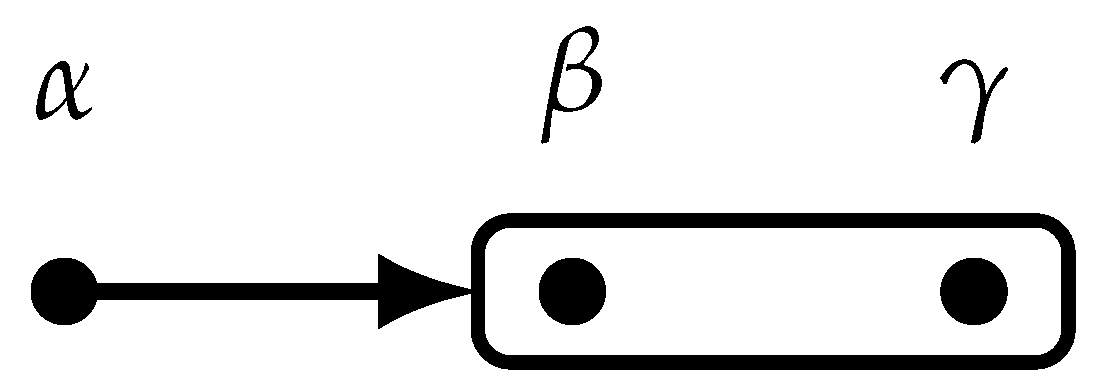
Graphically, we represent a transitive and euclidean belief relation as shown in Figure 4, where ${\omega }^{\prime }\in \mathcal{B}\left(\omega \right)$ if and only if either there is an arrow from $\omega$ to the rounded rectangle containing ${\omega }^{\prime }$, or $\omega$ and ${\omega }^{\prime }$ are enclosed in the same rounded rectangle (that is, if there is an arrow from state $\omega$ to a rounded rectangle, then, for every ${\omega }^{\prime }$ in that rectangle, $(\omega ,{\omega }^{\prime })\in \mathcal{B}$ and, for any two states $\omega$ and ${\omega }^{\prime }$ that are enclosed in a rounded rectangle, $\{(\omega ,\omega ),(\omega ,{\omega }^{\prime }),({\omega }^{\prime },\omega ),({\omega }^{\prime },{\omega }^{\prime })\}\subseteq \mathcal{B}$).

The object of beliefs are propositions or events (i.e., sets of states; events are denoted by bold-type capital letters). We say that at state ω the agent believes event $\mathbf{E}\subseteq \mathrm{\Omega }$ if and only if $\mathcal{B}\left(\omega \right)\subseteq \mathbf{E}$. For example, in the case illustrated in Figure 4, at state $\alpha$ the agent believes event $\{\beta ,\gamma \}$. We say that, at state ω, event $\mathbf{E}$ is true if $\omega \in \mathbf{E}$. In the case illustrated in Figure 4, at state $\alpha$ the agent erroneously believes event $\{\beta ,\gamma \}$, since event $\{\beta ,\gamma \}$ is not true at $\alpha$ ($\alpha \notin \mathcal{B}\left(\alpha \right)=\{\beta ,\gamma \}$). We say that at state ω the agent has correct beliefs if $\omega \in \mathcal{B}\left(\omega \right)$ (note that it is a consequence of euclideanness of the relation $\mathcal{B}$ that, even if the agent’s beliefs are objectively incorrect, she always believes that what she believes is true: if ${\omega }^{\prime }\in \mathcal{B}\left(\omega \right)$ then ${\omega }^{\prime }\in \mathcal{B}\left({\omega }^{\prime }\right)$).

3.2. Models of Games

As a starting point in the definition of a model of a game, we take a set of states $\mathrm{\Omega }$ and provide an interpretation of each state in terms of a particular play of the game, by means of a function $\zeta :\mathrm{\Omega }\to Z$ that associates, with every state $\omega$, a play or terminal history $\zeta \left(\omega \right)\in Z$. Each state $\omega$ also provides a description of the beliefs of the active players by means of a binary relation ${\mathcal{B}}_h$ on $\mathrm{\Omega }$ representing the beliefs of $\iota \left(h\right)$, the player who moves at decision history h. It would be more precise to write ${\mathcal{B}}_{\iota \left(h\right)}$ instead of ${\mathcal{B}}_h$, but we have chosen the lighter notation since there is no ambiguity, because we assume (see Appendix A) that at every decision history there is a unique player who is active there. Note that beliefs are specified only at histories that are reached at a given state, in the sense that ${\mathcal{B}}_h\left(\omega \right)\ne ⌀$ if and only if $h\prec \zeta \left(\omega \right)$.

Definition 1. 

A model of an extensive-form game is a tuple $〈\mathrm{\Omega },\zeta ,{\left\{{\mathcal{B}}_h\right\}}_{h\in D}〉$ where

• Ω is a set of states.
• $\zeta :\mathrm{\Omega }\to Z$ is an assignment of a terminal history to each state.
• For every $h\in D$, ${\mathcal{B}}_h\subseteq \mathrm{\Omega }\times \mathrm{\Omega }$ is a belief relation that satisfies the following properties:

  1.

  ${\mathcal{B}}_h\left(\omega \right)\ne ⌀$ if and only if $h\prec \zeta \left(\omega \right)$ [beliefs are specified only at reached decision histories and are consistent: consistency means that there is no event $\mathbf{E}$ such that both $\mathbf{E}$ and its complement $\neg \mathbf{E}$ are believed; it is well known that, at state ω, beliefs are consistent if and only if $\mathcal{B}\left(\omega \right)\ne ⌀$].

  2.

  If ${\omega }^{\prime }\in {\mathcal{B}}_h\left(\omega \right)$ then $h^{\prime }\prec \zeta \left({\omega }^{\prime }\right)$ for some $h^{\prime }$ such that $h^{\prime }{\approx }_{\iota \left(h\right)}h$ [the active player at history h correctly believes that her information set that contains h has been reached; recall (see Appendix A) that $h^{\prime }{\approx }_{\iota \left(h\right)}h$ (also written as $h^{\prime }\in \left[h\right]$) if and only if h and $h^{\prime }$ belong to the same information set of player $\iota \left(h\right)$ (thus $\iota \left(h\right)=\iota \left(h^{\prime }\right))$].

  3.

  If ${\omega }^{\prime }\in {\mathcal{B}}_h\left(\omega \right)$ then (1) ${\mathcal{B}}_h\left({\omega }^{\prime }\right)={\mathcal{B}}_h\left(\omega \right)$ and (2) if $h^{\prime }\prec \zeta \left({\omega }^{\prime }\right)$ with $h^{\prime }{\approx }_{\iota \left(h\right)}h$ then ${\mathcal{B}}_{h^{\prime }}\left({\omega }^{\prime }\right)={\mathcal{B}}_h\left(\omega \right)$ [by (1), beliefs satisfy positive and negative introspection and, by (2), beliefs are the same at any two histories in the same information set; thus one can unambiguously refer to a player’s beliefs at an information set, which is what we do in Figures 5–9].

  4.

  If ${\omega }^{\prime }\in {\mathcal{B}}_h\left(\omega \right)$ and $h^{\prime }\prec \zeta \left({\omega }^{\prime }\right)$ with $h^{\prime }{\approx }_{\iota \left(h\right)}h$, then, for every action $a\in A\left(h\right)$ (note that $A\left(h^{\prime }\right)=A\left(h\right)$), there is an ${\omega }^{″}\in {\mathcal{B}}_h\left(\omega \right)$ such that $h^{\prime }a\precsim \zeta \left({\omega }^{″}\right)$.

The last condition states that if, at state $\omega$ and history h reached at $\omega$ ($h\prec \zeta \left(\omega \right)$), player $\iota \left(h\right)$ considers it possible that the play of the game has reached history $h^{\prime }$, which belongs to her information set that contains h, then, for every action a available at that information set, there is a state ${\omega }^{″}$ that she considers possible at h and $\omega$ (${\omega }^{″}\in {\mathcal{B}}_h\left(\omega \right)$) where she takes action a at history $h^{\prime }$ ($h^{\prime }a\precsim \zeta \left({\omega }^{″}\right)$). This means that, for every available action, the active player at h considers it possible that she takes that action and thus has a belief about what will happen conditional on taking it. A further “natural” restriction on beliefs will be discussed later (Definition 6).

Figure 5 reproduces the game of Figure 1 and shows a model of it. For every reached decision history, under every state that the corresponding player considers possible we have shown the action actually taken by that player and the player’s payoff (at the terminal history associated with that state).

Suppose, for example, that the actual state is $\gamma$. State $\gamma$ encodes the following facts and beliefs.

1.

As a matter of fact, Player 1 plays a, Player 2 plays b and Player 3 plays d.

2.

Player 1 (who chooses at the null history ⌀) believes that if she plays a then Player 2 will also play a (this belief is erroneous since at state $\gamma$ Player 2 actually plays b, after Player 1 plays a) and thus her utility will be 2, and she believes that if she plays b then Player 2 will play a and Player 3 will play d and thus her utility will be 1.

3.

Player 2 (who chooses at information set $\{a,b\}$) correctly believes that Player 1 played a and, furthermore, correctly believes that if he plays b then Player 3 will play d and thus his utility will be 1, and believes that if he plays a his utility will be 2.

4.

Player 3 (who chooses at information set $\{ab,ba,bb\}$) erroneously believes that both Player 1 and Player 2 played b; thus, she believes that if she plays c her utility will be 0 and if she plays d her utility will be 1.

On the other hand, if the actual state is $\beta$, then the actual play is $aa$ and the beliefs of Players 1 and 2 are as detailed above (Points 2 and 3, respectively), while no beliefs are specified for Player 3, because Player 3 does not get to play (that is, Player 3 is not active at state $\beta$ since her information set is not reached).

3.3. Rationality

Consider again the model of Figure 5 and state $\gamma$. There Player 1 believes that if she takes action a, her utility will be 2, and if she takes action b, her utility will be 1. Thus, if she is rational, she must take action a. Indeed, at state $\gamma$ she does take action a and thus she is rational (although she will later discover that her belief was erroneous and the outcome turns out to be $abd$ not $aa$ so that her utility will be 1, not 2). Since Player 1 has the same beliefs at every state, we declare Player 1 to be rational at precisely those states where she takes action a, namely $\beta$ and $\gamma$. Similar reasoning leads us to conclude that Player 2 is rational at those states where she takes action a, namely states $\alpha$ and $\beta$. Similarly, Player 3 is rational at those states where she takes action d, namely states $\alpha$, $\gamma$ and $\delta$. If we denote by $\mathbf{R}$ the event that all the active players are rational, then in the model of Figure 5 we have that $\mathbf{R}=\left\{\beta \right\}$ (note that at state $\beta$ Player 3 is not active).

We need to define the notion of rationality more precisely. Various definitions of rationality have been suggested in the context of extensive-form games, most notably material rationality and substantive rationality [28,29]. The notion of material rationality is the weaker of the two in that a player can be found to be irrational only at decision histories of hers that are actually reached (substantive rationality, on the other hand, is more demanding since a player can be labeled as irrational at a decision history h of hers even if h not reached). Given that we have adopted a purely behavioral approach, the natural notion for us is the weaker one, namely material rationality. We will adopt a very weak version of it, according to which at a state $\omega$ and reached history h (that is, $h\prec \zeta \left(\omega \right)$), the active player at h is rational if the following is the case: if a is the action that the player takes at h at state $\omega$ (that is, $ha\precsim \zeta \left(\omega \right)$) then there is no other action at h that, according to her beliefs, guarantees a higher utility.

Definition 2. 

Let ω be a state, h a decision history that is reached at ω ($h\prec \zeta \left(\omega \right)$) and $a,b\in A\left(h\right)$ two actions available at h.

(A) 

We say that, at ω and h, the active player $\iota \left(h\right)$ believes that b is better than a if, for all ${\omega }_1,{\omega }_2\in {\mathcal{B}}_h\left(\omega \right)$ and for all $h^{\prime }$ such that $h^{\prime }{\approx }_{\iota \left(h\right)}h$ (that is, history $h^{\prime }$ belongs to the same information set as h), if a is the action taken at history $h^{\prime }$ at state ${\omega }_1$, that is, $h^{\prime }a\precsim \zeta \left({\omega }_1\right)$, and b is the action taken at $h^{\prime }$ at state ${\omega }_2$, that is, $h^{\prime }b\precsim \zeta \left({\omega }_2\right)$, then $u_{\iota \left(h\right)}\left(\zeta \left({\omega }_1\right)\right)<u_{\iota \left(h\right)}\left(\zeta \left({\omega }_2\right)\right)$. Thus, the active player at history h believes that action b is better than action a if, restricting attention to the states that she considers possible, the largest utility that she obtains if she plays a is less than the lowest utility that she obtains if she plays b.

(B) 

We say that player $\iota \left(h\right)$ is rational at history h at state ω if and only if the following is true: if $ha\precsim \zeta \left(\omega \right)$ (that is, $a\in A\left(h\right)$ is the action played at h at state ω) then, for every $b\in A\left(h\right)$, it is not the case that, at state ω and history h, player $\iota \left(h\right)$ believes that b is better than a.

Finally, we define the event that all the active players are rational, denoted by $\mathbf{R}$ as follows:

$$\begin{array}{c}\omega \in \mathbf{R}\mathrm{if}\mathrm{and}\mathrm{only}\mathrm{if},\mathrm{for}\mathrm{every}h\prec \zeta \left(\omega \right),\hfill \\ \mathrm{player}\iota \left(h\right)\mathrm{is}\mathrm{rational}\mathrm{at}h\left(\mathrm{at}\mathrm{state}\omega \right).\hfill \end{array}$$

(1)

For example, as noted above, in the model of Figure 5 we have that $\mathbf{R}=\left\{\beta \right\}$.

3.4. Correct Beliefs

The notion of correct belief was first mentioned in Section 3.1 and was identified with local reflexivity (that is, reflexivity at a state, rather than global reflexivity). Since, at any state, only the beliefs of the active players are specified, we define the event that players have correct beliefs by restricting attention to those players who actually move. Thus, the event that the active players have correct beliefs, denoted by $\mathbf{T}$ (‘T’ stands for ‘true’), is defined as follows:

$$\omega \in \mathbf{T}\mathrm{if}\mathrm{and}\mathrm{only}\mathrm{if}\omega \in {\mathcal{B}}_h\left(\omega \right)\mathrm{for}\mathrm{every}h\mathrm{such}\mathrm{that}h\prec \zeta \left(\omega \right).$$

(2)

For example, in the model of Figure 5, $\mathbf{T}=\left\{\beta \right\}$.

What does the expression “correct beliefs” mean? Consider state $\beta$ in the model of Figure 5 where the active players (Players 1 and 2) have correct beliefs in the sense of (2) ($\beta \in {\mathcal{B}}_{⌀}\left(\beta \right)$ and $\beta \in {\mathcal{B}}_{\{a,b\}}\left(\beta \right)$). Consider Player 1. There are two components to Player 1’s beliefs: (i) she believes that if she plays a then Player 2 will also play a, and ($ii$) she believes that if she plays b then Players 2 and 3 will play a and d, respectively. The first belief is correct at state $\beta$, where Player 1 plays a and Player 2 indeed follows with a. As for the second belief, whether it is correct or not depends on how we interpret it. If we interpret it as the material conditional “if b then $bad$” (which is equivalent to “either not b or $bad$”) then it is indeed true at state $\beta$, but trivially so, because the antecedent is false there (Player 1 does not play b). If we interpret it as a counterfactual conditional “if Player 1 were to play b then Players 2 and 3 would play a and d, respectively” then in order to decide whether the conditional is true or not one would need to enrich the model by adding a “similarity” or “closeness” relation on the set of states (in the spirit of [3,4]); one would then check if at the closest state(s) to $\beta$ at which Player 1 plays b it is indeed the case that Players 2 and 3 play a and d, respectively. Note that there is no a priori reason to think that the closest state to $\beta$ where Player 1 plays b is state $\alpha$. This is because, as pointed out by Stalnaker ([30], p.48), there is no necessary connection between counterfactuals, which capture causal relations, and beliefs: for example, I may believe that, if I drop the vase that I am holding in my hands, it will break (because I believe it is made of glass) but my belief is wrong because—as a matter of fact—if I were to drop it, it would not break, since it is made of plastic.

Our models do not have the resources to answer the question: “at state $\beta$, is it true —as Player 1 believes—that if Player 1 were to play b then Players 2 and 3 would play a and d, respectively?” One could, of course, enrich the models in order to answer the question, but is there a compelling reason to do so? In other words, is it important to be able to answer such questions? If we are merely interested in determining what rational players do, then what matters is what actions they actually take and what they believe when they act, whether or not those beliefs are correct in a stronger sense than is captured by the material conditional.

Is the material conditional interpretation of “if I play a then the outcome will be x” sufficient, though? Since the crucial assumption in the proposed framework is that the agent considers all of her available actions as possible (that is, for every available action there is a doxastically accessible state where she takes that action), material conditionals are indeed sufficient: the material conditional “if I take action a the outcome will be x” zooms in—through the lens of the agent’s beliefs— on those states where action a is indeed taken and verifies that at those states the outcome is indeed x, while the states where action a is not taken are not relevant for the truth of the conditional.

3.5. Self-Confirming Play

We have defined two events: the event $\mathbf{R}$ that all the active players are rational and the event $\mathbf{T}$ that all the active players have correct beliefs. In the model of Figure 5 we have that $\mathbf{R}\cap \mathbf{T}=\left\{\beta \right\}$ and it so happens that $\zeta \left(\beta \right)=aa$ is a Nash equilibrium play, that is, there is a pure-strategy Nash equilibrium (namely, $(a,a,d)$) whose associated play is $aa$. However, as shown below, this is not always the case.

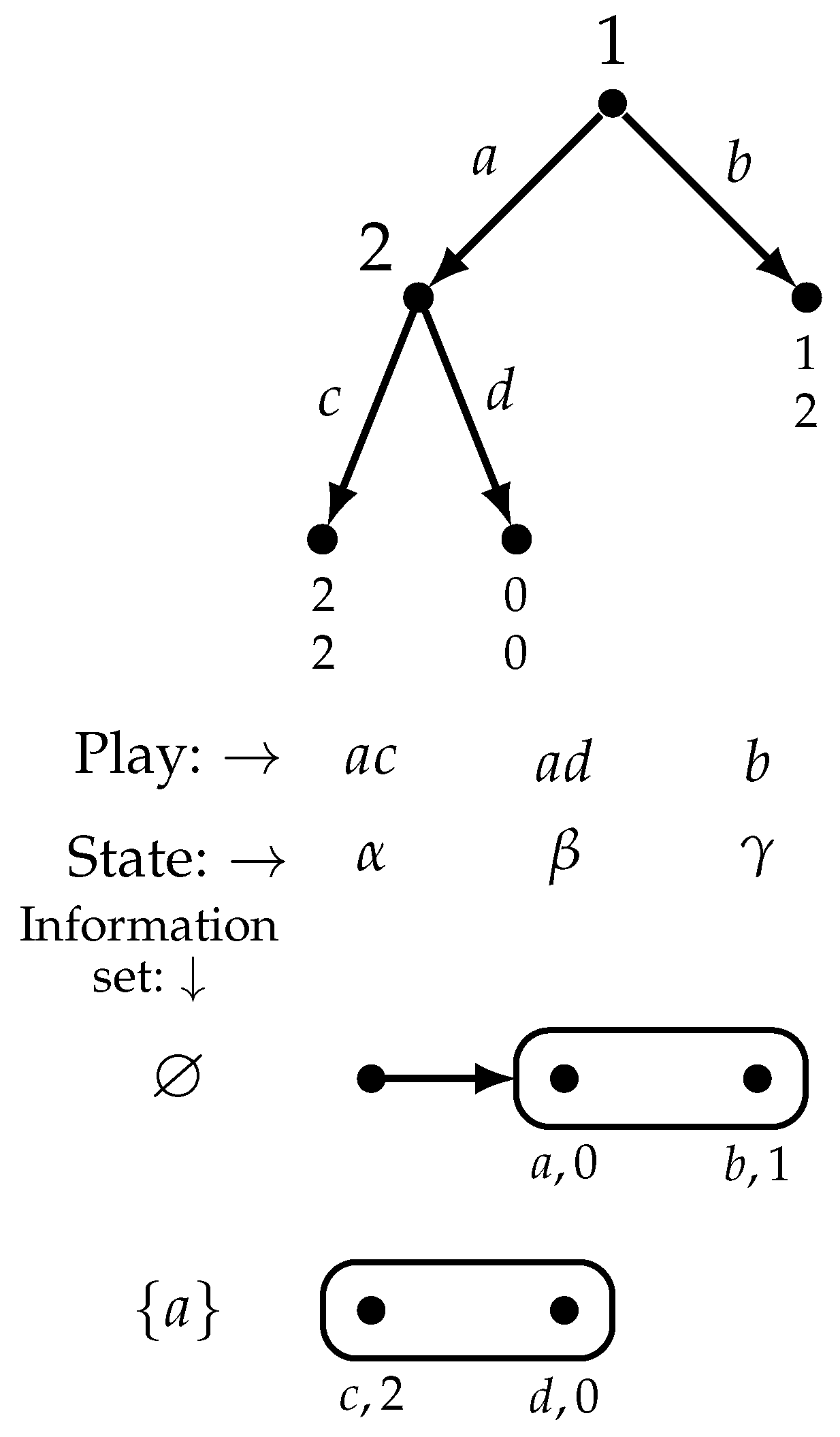
At a play associated with a state $\omega \in \mathbf{R}\cap \mathbf{T}$, each active player’s chosen action is rationally justified by her beliefs at the time of choice (since $\omega \in \mathbf{R}$) and the beliefs concerning what will happen after that action turn out to be correct (since $\omega \in \mathbf{T}$), so that no player is faced with evidence that her beliefs were wrong. Does that mean that, once the final outcome $\zeta \left(\omega \right)$ is revealed, no player regrets her actual choice? The answer is negative, because it is possible that a player, while not having any false beliefs, might not anticipate with precision the actions of the players who move after her. In the model shown in Figure 6 we have that $\mathbf{R}\cap \mathbf{T}=\{\alpha ,\beta ,\gamma \}$, that is, at every state the active players are rational and have correct beliefs. Consider state $\beta$, where the play is $ad$. At state $\beta$ Player 1 is rational because she believes that if she plays b her utility will be 1 and if she plays a her utility might be 0 but might also be 2 (she is uncertain about what Player 2 will do). Thus, she does not believe that action b is better than a and hence it is rational for her to play a (Definition 2). Player 2 is rational because she is indifferent between her two actions. However, ex post, when Player 1 learns that the actual outcome is $ad$, she regrets not taking action b instead of a. This example shows that, even though $\beta \in \mathbf{R}\cap \mathbf{T}$, $\zeta \left(\beta \right)=ad$ is not a Nash equilibrium play, that is, there is no Nash equilibrium whose associated play is $ad$.

Next we introduce another event which, in conjunction with $\mathbf{T}$, guarantees that the active players’ beliefs about the opponents’ actual moves are exactly correct (note that a requirement built in the definition of a self-fulfilling equilibrium ([13], p.523) is that “each player’s beliefs about the opponents’ play are exactly correct”). Event $\mathbf{C}$ (’C’ for ’certainty’) defined below rules out uncertainty about the opponents’ past choices (Point 1) as well as uncertainty about the opponents’ future choices (Point 2). Note that Point 1 is automatically satisfied in games with perfect information and thus imposes restrictions on beliefs only in imperfect-information games.

Definition 3. 

A state ω belongs to event $\mathbf{C}$ if and only if, for every reached history h at ω (that is, for every $h\prec \zeta \left(\omega \right))$, and $\forall {\omega }^{\prime },{\omega }^{″}\in {\mathcal{B}}_h\left(\omega \right)$, $\forall h^{\prime },h^{″}\in \left[h\right]$ (recall that $\left[h\right]$ is the information set that contains h),

1.

if $h^{\prime }\prec \zeta \left({\omega }^{\prime }\right)$ and $h^{″}\prec \zeta \left({\omega }^{″}\right)$ then $h^{\prime }=h^{″}$,

2.

$\forall a\in A\left(h\right)$, if $h^{\prime }a\prec \zeta \left({\omega }^{\prime }\right)$ and $h^{″}a\prec \zeta \left({\omega }^{″}\right)$ then $\zeta \left({\omega }^{\prime }\right)=\zeta \left({\omega }^{″}\right)$.

Note that—concerning Point 1—a player may be erroneous in her certainty about the opponents’ past choices, that is, it may be that $\omega \in \mathbf{C}$, the actual reached history is $h\prec \zeta \left(\omega \right)$ and yet player $\iota \left(h\right)$ is certain that she is moving at history $h^{\prime }\in \left[h\right]$ with $h^{\prime }\ne h$ (for example, in the model of Figure 5, at state $\gamma$, which belongs to event $\mathbf{C}$, and at reached history $ab$, Player 3 is certain that she is moving at history $bb$ while, as a matter of fact, she is moving at history $ab$), and—concerning Point 2— a player may also be erroneous in her certainty about what will happen after her choice (for example, in the model of Figure 5, at state $\mathrm{\gamma }$ and history ⌀, Player 1 is certain that if she takes action a then Player 2 will also play a, but she is wrong about this, because, as a matter of fact, at state $\mathrm{\gamma }$ Player 2 follows with b rather than a).

In the model of Figure 5 $\mathbf{C}=\mathrm{\Omega }$, while in the model of Figure 6 $\mathbf{C}=⌀$, because at the null history ⌀ Player 1 is uncertain about what will happen if she takes action a.

If state $\omega$ belongs to the intersection of events $\mathbf{C}$ and $\mathbf{T}$ then, at state $\omega$, each active player’s beliefs about the opponents’ actual play are exactly correct. Note, however, that—as noted in Section 3.4—there is no way of telling whether or not a player is also correct about what would happen after her counterfactual choices, because the models that we are considering are not rich enough to address the issue of counterfactuals.

Definition 4. 

Let G be a game and z a play (or terminal history) in G. We say that z is a self-confirming play if there exists a model of G and a state ω in that model such that (1) $\omega \in \mathbf{R}\cap \mathbf{T}\cap \mathbf{C}$ and (2) $z=\zeta \left(\omega \right)$.

Definition 5. 

Given a game G and a play z in G, call z a Nash play if there is a pure-strategy Nash equilibrium whose induced play is z.

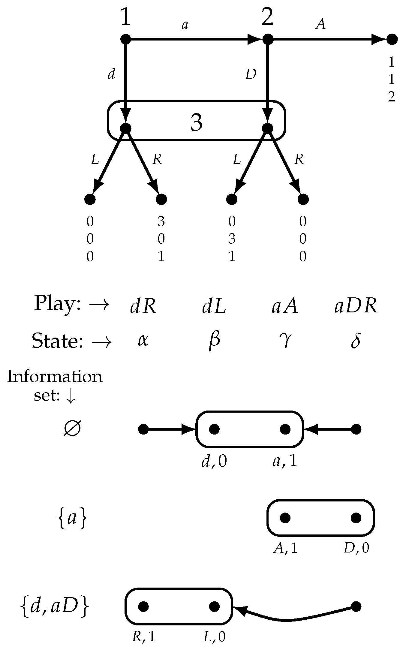
It turns out that, in perfect-information games in which no player moves more than once along any play, the two notions of self-confirming play and Nash play are equivalent ([1], Proposition 1, p. 1012). For games with imperfect information, while it is still true that a Nash play is a self-confirming play, there may be self-confirming plays that are not Nash plays. The reason for this is that two players might have different beliefs about the potential choice of a third player. Figure 7 reproduces the game of Figure 3 together with a model of it.

In the model of Figure 7, $\mathbf{R}=\left\{\mathrm{\gamma }\right\}$, $\mathbf{T}=\{\beta ,\mathrm{\gamma }\}$ and $\mathbf{C}=\mathrm{\Omega }$, so that $\mathbf{R}\cap \mathbf{T}\cap \mathbf{C}=\left\{\mathrm{\gamma }\right\}$. Thus, at state $\mathrm{\gamma }$ the active players (Players 1 and 2) are rational, have correct beliefs and have no uncertainty and yet $\zeta \left(\mathrm{\gamma }\right)=aA$ which is not a Nash play (there is no Nash equilibrium that yields the play $aA$). Players 1 and 2 have different beliefs about what Player 3 would do at her information set: at state $\mathrm{\gamma }$ Player 1 believes that if she plays d then Player 3 will play L, while Player 2 believes that if he plays D then Player 3 will play R.

Next we introduce a new event, denoted by $\mathbf{A}$ (‘A’ stands for ‘agreement’), that rules out such disagreement and use it to provide a doxastic characterization of Nash play in general games (with possibly imperfect information). First we need to add one more condition to the definition of a model of a game that is relevant only if the game has imperfect information.

The definition of model given in Section 3 (Definition 1) allows for “unreasonable” beliefs that express a causal link between a player’s action and her opponent’s reaction to it, when the latter does not observe the former’s choice. As an illustration of such beliefs, consider a game where Player 1 moves first, choosing between actions a and b, and Player 2 moves second choosing between actions c and d without being informed of Player 1’s choice, that is, histories a and b belong to the same information set of Player 2. Definition 1 allows Player 1 to have the following beliefs: “if I play a, then Player 2 will play c, while if I play b then Player 2 will play d”. Such beliefs ought to be rejected as “irrational” on the grounds that there cannot be a causal link between Player 1’s move and Player 2’s choice, since Player 2 does not get to observe Player 1’s move and thus cannot react differently to Player 1’s choice of a and Player 1’s choice of b. [It should be noted, however, that several authors have argued that such beliefs are not necessarily irrational: see, for example, [31,32,33,34,35,36]. A “causally correct” belief for Player 1 would require that the predicted choice(s) of Player 2 be the same, no matter what action Player 1 herself chooses.

Definition 6. 

A causally restricted model of a game is a model (Definition 1) that satisfies the following additional restriction (a verbal interpretation follows; note that, for games with perfect information, there is no difference between a model and a restricted model, since (3) is vacuously satisfied).

5. 

Let ω be a state, h a decision history reached at ω ($h\prec \zeta \left(\omega \right)$) and a and b two actions available at h ($a,b\in A\left(h\right)$). Let $h_1$ and $h_2$ be two decision histories that belong to the same information set of player $j=\iota \left(h_1\right)$ ($h_1{\approx }_j{h}_2$) and $c_1,c_2$ be two actions available at $h_1$ ($c_1,c_2\in A\left(h_1\right)=A\left(h_2\right)$). Then the following holds (recall that $\left[h\right]$ denotes the information set that contains decision history h, that is, $h^{\prime }\in \left[h\right]$ if and only if $h^{\prime }{\approx }_{\iota \left(h\right)}h$):

$$\begin{array}{c}\mathit{if}{h}^{\prime },h^{″}\in \left[h\right],{\omega }_1,{\omega }_2\in {\mathcal{B}}_h\left(\omega \right),h^{\prime }a\prec h_1{c}_1\precsim \zeta \left({\omega }_1\right)\mathit{and}\hfill \\ h^{″}b\prec h_2{c}_2\precsim \zeta \left({\omega }_2\right),\mathit{then}\mathit{either}{c}_1=c_2\mathit{or}\mathit{there}\mathit{exist}\hfill \\ {\omega }_1^{\prime },{\omega }_2^{\prime }\in {\mathcal{B}}_h\left(\omega \right)\mathit{such}\mathit{that}{h}^{\prime }a\prec h_1{c}_2\precsim \zeta \left({\omega }_1^{\prime }\right)\mathit{and}\hfill \\ h^{″}b\prec h_2{c}_1\precsim \zeta \left({\omega }_2^{\prime }\right).\hfill \end{array}$$

(3)

In words: if, at state $\omega$ and reached history h, player $i=\iota \left(h\right)$ considers it possible that, if she takes action a, history $h_1$ is reached and player $j=\iota \left(h_1\right)$ takes action $c_1$ at $h_1$ and player i also considers it possible that, if she takes action b, then history $h_2$ is reached, which belongs to the same information set as $h_1$, and player j takes action $c_2$ at $h_2$, then either $c_1=c_2$ or at state $\omega$ and history h player i must also consider it possible that (1) after taking action a, $h_1$ is reached and player j takes action $c_2$ at $h_1$ and (2) after taking action b, $h_2$ is reached and player j takes action $c_1$ at $h_2$.

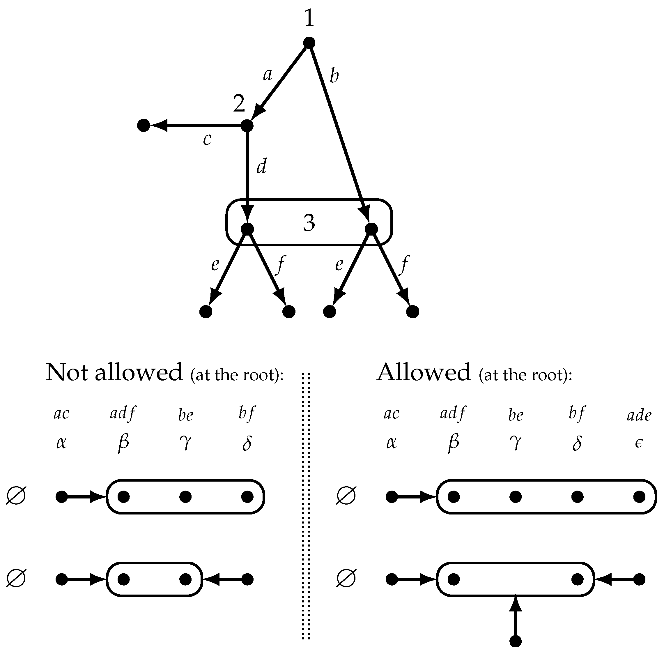
Figure 8 shows a game and four partial models of it, giving only the beliefs of Player 1 (at history ⌀): two of them violate Condition 5 of Definition 6 (the ones on the left that are labeled “not allowed”), while the other two satisfy it. Note that the models shown in Figure 5, Figure 6 and Figure 7 are all causally restricted models.

Now we turn to the notion of agreement, which is intended to rule out situations like the one shown in Figure 7 where Players 1 and 2 disagree about what action Player 3 would take at her information set $\{d,aD\}$.

Definition 7. 

We say that at state ω active players i and j consider future information set $\left[h\right]$ of player $k=\iota \left(h\right)$ if there exist

1.

two decision histories $h_1$ and $h_2$ that are reached at ω (that is, $h_1\prec h_2\prec \zeta \left(\omega \right)$) and belong to i and j, respectively, (that is, $i=\iota \left(h_1\right)$ and $j=\iota \left(h_2\right)$),

2.

states ${\omega }_1\in {\mathcal{B}}_{h_1}\left(\omega \right)$ and ${\omega }_2\in {\mathcal{B}}_{h_2}\left(\omega \right)$,

3.

decision histories $h^{\prime },h^{″}\in \left[h\right]$,

such that, for some $h_1^{\prime }{\approx }_i{h}_1$, $h_1^{\prime }\prec h^{\prime }\prec \zeta \left({\omega }_1\right)$ and, for some $h_2^{\prime }{\approx }_j{h}_2$, $h_2^{\prime }\prec h^{″}\prec \zeta \left({\omega }_2\right)$.

That is, player i at $h_1$ considers it possible that the play has reached history $h_1^{\prime }\in \left[h_1\right]$ and, after taking an action at $h_1^{\prime }$, information set $\left[h\right]$ of player k is reached, and player j at $h_2$ considers it possible that the play has reached history $h_2^{\prime }\in \left[h_2\right]$ and, after taking an action at $h_2^{\prime }$, that same information set $\left[h\right]$ of player k is reached.

Definition 8. 

We say that at state ω active players i and j are in agreement if, for every future information set $\left[h\right]$ that they consider (Definition 7), they predict the same choices(s) of player $k=\iota \left(h\right)$ at h, that is, if player i is active at reached history $h_1$ and player j is active at reached history $h_2$, with $h_1\prec h_2\prec \zeta \left(\omega \right)$, then

1.

if ${\omega }_1\in {\mathcal{B}}_{h_1}\left(\omega \right)$ and $h_1^{\prime }\prec h^{\prime }a\precsim \zeta \left({\omega }_1\right)$ with $h_1^{\prime }\in \left[h_1\right]$, $h^{\prime }\in \left[h\right]$ and $a\in A\left(h\right)$, then there exists an ${\omega }_2\in {\mathcal{B}}_{h_2}\left(\omega \right)$ such that, for some $h^{″}\in \left[h\right]$ and $h_2^{\prime }\in \left[h_2\right]$, $h_2^{\prime }\prec h^{″}a\precsim \zeta \left({\omega }_2\right)$, and

2.

if ${\omega }_2\in {\mathcal{B}}_{h_2}\left(\omega \right)$ with $h_2^{\prime }\prec h^{″}b\precsim \zeta \left({\omega }_2\right)$ with $h_2^{\prime }\in \left[h_2\right]$, $h^{″}\in \left[h\right]$ and $b\in A\left(h\right)$ then here exists an ${\omega }_1\in {\mathcal{B}}_{h_1}\left(\omega \right)$ such that, for some $h^{\prime }\in \left[h\right]$ and $h_1^{\prime }\in \left[h_1\right]$, $h_1^{\prime }\prec h^{\prime }b\precsim \zeta \left({\omega }_1\right)$.

Finally we define the event, denoted by $\mathbf{A}$, that any two active players are in agreement:

$$\omega \in \mathbf{A}\mathrm{if}\mathrm{and}\mathrm{only}\mathrm{if}\mathrm{any}\mathrm{two}\mathrm{players}\mathrm{active}\mathrm{at}\omega \mathrm{are}\mathrm{in}\mathrm{agreement}\mathrm{at}\omega .$$

(4)

We can now state our characterization result, according to which a self-confirming play is a Nash play if and only if the beliefs of any two players are in agreement about the hypothetical choice(s) of a third player at a future information set that they both consider. As in [1] we restrict attention to games that satisfy the property that each player moves at most once along any play. Equivalently, one could consider the agent form of the game, where the same player at different information sets is regarded as different players, but with the same payoff function.

Proposition 1. 

Consider a finite extensive-form game G where no player moves more than once along any play. Then,

(A) 

If z is a Nash play of G then there is a causally restricted model of G and a state $\omega$ in that model such that (1) $\zeta \left(\omega \right)=z$ and (2) $\omega \in \mathbf{R}\cap \mathbf{T}\cap \mathbf{C}\cap \mathbf{A}$.

(B) 

For any causally restricted model of G and for every state $\omega$ in that model, if $\omega \in \mathbf{R}\cap \mathbf{T}\cap \mathbf{C}\cap \mathbf{A}$ then $\zeta \left(\omega \right)$ is a Nash play.

The proof of Proposition 1 is given in Appendix B.

Note that, in a perfect-information game, $\mathbf{T}\cap \mathbf{C}\subseteq \mathbf{A}$. Hence Proposition 1 in [1] is a corollary of the above Proposition.

4. Further Discussion and Conclusions

A reviewer suggested a discussion of the similarities and differences between the approach put forward in this paper and Steven Brams’ Theory of Moves (TOM) [37] (see also the very recent [38]). TOM deals mostly with two-person strategic-form games in which each player has a strict ordinal ranking of the outcomes. TOM assumes that, instead of choosing strategies simultaneously and independently, players start from an outcome (that is, a strategy profile)—called the “initial state”—and from that outcome they consider the consequences of a series of moves and countermoves that lead from state to state. The sequence of moves and countermoves is strictly alternating and the process continues until the game terminates in a “final state” which is called the “final outcome” or simply “outcome” of the game. It is assumed that no payoffs accrue to players from being in a state unless it is the final state (which could be the initial state if the players choose not to move from it). Players make farsighted calculations of where play will terminate after a finite sequence of moves and countermoves. The result of such farsighted calculations is called a Non-Myopic Equilibrium (NME). Thus, an NME can be understood as the backward-induction solution of a finite perfect-information “moves game” (with no ties).

There are two points in common between TOM and our approach. First of all, only ordinal preferences are considered in both approaches. Secondly, both approaches are based on a departure from standard solution concepts in game theory. However, the differences between the two approaches are substantial. Brams’ theory is not based at all on epistemic considerations: no beliefs are attributed to the players and the conceptual nature of a “state” is very different; in TOM a state is merely an outcome, while in our doxastic approach a state is described not only in terms of an outcome but also in terms of doxastic relations that describe what the active players believe about the possible outcomes when it is their turn to move. Furthermore, while TOM starts from a strategic-form game and builds on it a finite perfect-information game by specifying an initial outcome and the rules for moves and countermoves from it, we analyze a given extensive-form game (with possibly imperfect information) without modifying it in any way. Our approach falls within the “epistemic foundations approach” in which beliefs play an essential role. TOM, on the other hand, is entirely “belief-free”.

In Section 2, we raised the question “what constitutes a rational solution of an extensive-form game?” Most of the epistemic game theory literature has gone in the direction of imposing more and more subtle and complex conditions on counterfactual beliefs and choices of the players at unreached information sets. We suggested going in the opposite direction, by focusing only on the actions and beliefs of the active players. Within this framework, a natural notion of rational play is captured by the definition of self-confirming play, where each action taken is justified by the beliefs held at the time of choice and those beliefs turn out to be exactly correct, so that no player receives information that contradicts those beliefs and thus experiences no regret. This approach is flexible enough to allow one to explore the epistemic foundations of standard solution concepts such as Nash equilibrium and backward induction (within the behavioral approach described in this paper, the epistemic conditions needed to obtain a characterization of backward induction in perfect information games, or a generalized version of it for a class of games with imperfect-information, are investigated in [1] and [9], respectively).

The characterization of Nash play given in Proposition 1—unlike characterizations of Nash equilibrium provided for strategic-form games (for a discussion of the relevant literature the reader is referred to ([1], Section 6))—does not require players to believe in each other’s rationality. This can be seen in the game and model shown in Figure 9, where $\mathbf{R}=\left\{\mathrm{\gamma }\right\}$, $\mathbf{T}=\{\beta ,\mathrm{\gamma }\}$ and $\mathbf{C}=\mathbf{A}=\{\alpha ,\beta ,\mathrm{\gamma }\}$, so that $\mathbf{R}\cap \mathbf{T}\cap \mathbf{C}\cap \mathbf{A}=\left\{\mathrm{\gamma }\right\}$ but at $\mathrm{\gamma }$ Player 1 does not believe that Player 2 is rational, because $\beta \in {\mathcal{B}}_{⌀}\left(\mathrm{\gamma }\right)$ and at $\beta$ Player 2 is not rational (she plays d believing that c gives her higher utility).

In Definition 4 we put forward the notion of self-confirming play, which is in the spirit of self-confirming equilibrium ([13]), but framed in behavioral terms and without making use of the notion of strategy. Whereas in perfect-information games the notion of self-confirming play is equivalent to the notion of Nash play, the equivalence does not extend to imperfect information games. Proposition 1 identified the additional restriction that is needed to characterize the set of Nash plays in games with imperfect information.

The main purpose of this paper was to show that one can go a long way in the analysis of rational play in extensive-form games without using the notion of strategy, that is, without the need to specify choices at all histories—even those that are not reached—and without the need to model players’ beliefs at unreached histories. We argued that the standard approach based on Nash equilibrium and its refinements is too ambitious in its goal to tackle the counterfactual behavior and beliefs of players at unreached histories and that there is no need to pursue this goal in order to have a theory of rational behavior in dynamic games.

In what directions can the approach discussed in this paper be further developed? One natural extension is to move from ordinal preferences to von Neumann-Morgenstern preferences and from qualitative beliefs to probabilistic beliefs; one would then, correspondingly, move from the very weak definition of rationality given in Definition 2 to the stronger definition of rationality as expected utility maximization. Another possible line of inquiry would be to identify the circumstances (if any) that would make the structures used in this paper inadequate and would require a full analysis in terms of counterfactuals (which in turn would require extending those structures by adding similarity relations among states, as explained in Section 3).

References

- Bonanno, G. Behavior and deliberation in perfect-information games: Nash equilibrium and backward induction. Int. J. Game Theory 2018, 47, 1001–1032. [Google Scholar] [CrossRef] [Green Version]
- Kreps, D.; Wilson, R. Sequential equilibrium. Econometrica 1982, 50, 863–894. [Google Scholar] [CrossRef]
- Lewis, D. Counterfactuals; Harvard University Press: Cambridge, MA, USA, 1973. [Google Scholar]
- Stalnaker, R. A theory of conditionals. In Studies in Logical Theory; Rescher, N., Ed.; Blackwell: Oxford, UK, 1968; pp. 98–112. [Google Scholar]
- Stalnaker, R.; Thomason, R. A semantical analysis of conditional logic. Theoria 1970, 36, 246–281. [Google Scholar]
- Perea, A. Backward induction Versus Forw. Induction Reason. Games 2010, 1, 168–188. [Google Scholar] [CrossRef] [Green Version]
- Perea, A. Belief in the opponents’ future rationality. Games Econ. Behav. 2014, 83, 231–254. [Google Scholar] [CrossRef]
- Baltag, A.; Smets, S.; Zvesper, J. Keep ’hoping’ for rationality: A solution to the backward induction paradox. Synthese 2009, 169, 301–333. [Google Scholar]
- Bonanno, G. A doxastic behavioral characterization of generalized backward induction. Games Econ. Behav. 2014, 88, 221–241. [Google Scholar]
- Battigalli, P.; Siniscalchi, M. Strong belief and forward induction reasoning. J. Econ. Theory 2002, 106, 356–391. [Google Scholar]
- Pearce, D. Rationalizable strategic behavior and the problem of perfection. Econometrica 1984, 52, 1029–1050. [Google Scholar]
- Meier, M.; Perea, A. Forward Induction in a Backward Inductive Manner. Technical Report, EPICENTER, Maastricht University. 2022. Available online: https://www.epicenter.name/Perea/Papers/BI-FI-procedure.pdf (accessed on 23 September 2022).
- Fudenberg, D.; Levine, D. Self-confirming equilibrium. Econometrica 1993, 61, 523–545. [Google Scholar]
- Battigalli, P.; Guaitoli, D. Conjectural equilibria and rationalizability in a game with incomplete information. In Decisions, Games and Markets; Battigalli, P., Montesano, A., Panunzi, F., Eds.; Kluwer Academic Publishers: Dordrecht, The Netherlands, 1997; pp. 97–124. [Google Scholar]
- Greenberg, J. The right to remain silent. Theory Decis. 2000, 48, 193–204. [Google Scholar]
- Greenberg, J.; Gupta, S.; Luo, X. Mutually acceptable courses of action. Econ. Theory 2009, 40, 91–112. [Google Scholar]
- Dekel, E.; Fudenberg, D.; Levine, D. Payoff information and self-confirming equilibrium. J. Econ. Theory 1999, 89, 165–185. [Google Scholar] [CrossRef] [Green Version]
- Dekel, E.; Fudenberg, D.; Levine, D. Subjective uncertainty over behavior strategies: A correction. J. Econ. Theory 2002, 104, 473–478. [Google Scholar] [CrossRef] [Green Version]
- Fudenberg, D.; Kamada, Y. Rationalizable partition-confirmed equilibrium. Theor. Econ. 2015, 10, 775–806. [Google Scholar]
- Battigalli, P. Comportamento Razionale ed Equilibrio nei Giochi e nelle Situazioni Strategiche. Unpublished Dissertation, Bocconi University, Milano, Italy, 1987. [Google Scholar]
- Gilli, M. Metodo Bayesiano e Aspettative nella Teoria dei Giochi e nella Teoria Economica. Unpublished Dissertation, Bocconi University, Milano, Italy, 1987. [Google Scholar]
- Halpern, J. Substantive rationality and backward induction. Games Econ. Behav. 2001, 37, 425–435. [Google Scholar]
- Samet, D. Hypothetical knowledge and games with perfect information. Games Econ. Behav. 1996, 17, 230–251. [Google Scholar] [CrossRef] [Green Version]
- Battigalli, P.; Di-Tillio, A.; Samet, D. Strategies and interactive beliefs in dynamic games. In Advances in Economics and Econometrics. Theory and Applications: Tenth World Congress, Volume 1; Acemoglu, D., Arellano, M., Dekel, E., Eds.; Cambridge University Press: Cambridge, UK, 2013; pp. 391–422. [Google Scholar]
- Bonanno, G. A dynamic epistemic characterization of backward induction without counterfactuals. Games Econ. Behav. 2013, 78, 31–43. [Google Scholar]
- Bonanno, G. The material conditional is sufficient to model deliberation. Erkenntnis. February 2021. ISSN 1572-8420. Available online: https://link.springer.com/article/10.1007/s10670-020-00357-7 (accessed on 23 September 2022).
- Stalnaker, R. Knowledge, belief and counterfactual reasoning in games. Econ. Philos. 1996, 12, 133–163. [Google Scholar]
- Aumann, R. Backward induction and common knowledge of rationality. Games Econ. Behav. 1995, 8, 6–19. [Google Scholar] [CrossRef]
- Aumann, R. On the centipede game. Games Econ. Behav. 1998, 23, 97–105. [Google Scholar] [CrossRef] [Green Version]
- Stalnaker, R. Belief revision in games: Forward and backward induction. Math. Soc. Sci. 1998, 36, 31–56. [Google Scholar] [CrossRef]
- Bicchieri, C.; Green, M. Symmetry arguments for cooperation in the Prisoner’s Dilemma. In The Logic of Strategy; Bicchieri, C., Jeffrey, R., Skyrms, B., Eds.; Oxford University Press: Oxford, UK, 1999; pp. 175–195. [Google Scholar]
- Gauthier, D. Morals by Agreement; Oxford University Press: Oxford, UK, 1986. [Google Scholar]
- Nozick, R. Newcomb’s problem and two principles of choice. In Essays in Honor of Carl G. Hempel: A Tribute on the Occasion of His Sixty-Fifth Birthday; Rescher, N., Ed.; Springer: Dordrecht, The Netherlands, 1969; pp. 114–146. [Google Scholar] [CrossRef]
- Spohn, W. Dependency equilibria and the causal structure of decision and game situations. Homo Oeconomicus 2003, 20, 195–255. [Google Scholar] [CrossRef]
- Spohn, W. Dependency equilibria. Philos. Sci. 2007, 74, 775–789. [Google Scholar] [CrossRef] [Green Version]
- Spohn, W. From Nash to dependency equilibria. In Logic and the Foundations of Game and Decision Theory—LOFT 8; Bonanno, G., Löwe, B., van der Hoek, W., Eds.; Springer: Berlin/Heidelberg, Germany, 2010; pp. 135–150. [Google Scholar]
- Brams, S.J. Theory of Moves; Cambridge University Press: Cambridge, UK, 1993. [Google Scholar]
- Brams, S.; Ismail, M. Every normal-form game has a Pareto-optimal nonmyopic equilibrium. Theory Decis. 2022, 92, 349–362. [Google Scholar] [CrossRef]
Figure 1.
An extensive game with imperfect information.
Figure 2.
The conflict between the backward-induction-based counterfactual and the forward-induction-based counterfactual encoded in Player 2’s strategy.
Figure 3.
The play is consistent with the notion of self-confirming equilibrium, even though there is no Nash equilibrium that yields .
Figure 4.
The relation .
Figure 5.
The top part reproduces the game of Figure 1 and the bottom part shows a model of it.
Figure 6.
A perfect-information game and a model of it.
Figure 7.
The game of Figure 3 and a model of it.
Figure 8.
A game and four partial models of it (showing only the beliefs of Player 1 at history ⌀), two of which violate Condition 5 of Definition 6 and the remaining two do not.
Figure 9.
but at Player 1 does not believe that Player 2 is rational.
Publisher’s Note: MDPI stays neutral with regard to jurisdictional claims in published maps and institutional affiliations. |
© 2022 by the author. Licensee MDPI, Basel, Switzerland. This article is an open access article distributed under the terms and conditions of the Creative Commons Attribution (CC BY) license (https://creativecommons.org/licenses/by/4.0/).
Share and Cite
MDPI and ACS Style
Bonanno, G. Rational Play in Extensive-Form Games. Games 2022, 13, 72. https://doi.org/10.3390/g13060072
AMA Style
Bonanno G. Rational Play in Extensive-Form Games. Games. 2022; 13(6):72. https://doi.org/10.3390/g13060072
Chicago/Turabian StyleBonanno, Giacomo. 2022. "Rational Play in Extensive-Form Games" Games 13, no. 6: 72. https://doi.org/10.3390/g13060072
APA StyleBonanno, G. (2022). Rational Play in Extensive-Form Games. Games, 13(6), 72. https://doi.org/10.3390/g13060072
Note that from the first issue of 2016, this journal uses article numbers instead of page numbers. See further details here.