Particle Recognition on Transmission Electron Microscopy Images Using Computer Vision and Deep Learning for Catalytic Applications

Abstract

Recognition and measuring particles on microscopy images is an important part of many scientific studies, including catalytic investigations. In this paper, we present the results of the application of deep learning to the automated recognition of nanoparticles deposited on porous supports (heterogeneous catalysts) on images obtained by transmission electron microscopy (TEM). The Cascade Mask-RCNN neural network was used. During the training, two types of objects were labeled on raw TEM images of ‘real’ catalysts: visible particles and overlapping particle projections. The trained neural network recognized nanoparticles in the test dataset with 0.71 precision and 0.72 recall for both classes of objects and 0.84 precision and 0.79 recall for visible particles. The developed model is integrated into the open-access web service ‘ParticlesNN’, which can be used by any researcher in the world. Instead of hours, TEM data processing per one image analysis is reduced to a maximum of a couple of minutes and the divergence of mean particle size determination is approximately 2% compared to manual analysis. The proposed tool encourages accelerating catalytic research and improving the objectivity and accuracy of analysis.

1. Introduction

Advanced microscopy techniques, such as transmission electron microscopy (TEM), are widely used in modern materials science, and in particularly in catalysis. In heterogeneous catalysis, the catalyst usually consists of an active component deposited as nanoparticles on a support [1,2,3,4,5,6]. The active component and porous supports can be of different nature but are commonly well suited to electron microscopy experiments [1,3,5]. TEM study is widely used during the preparation of catalysts, developing approaches to morphology, composition control, and ways to support particle stabilization [1,3,5,6], investigation of size effects in catalytic activity [4], ‘particle–support’ interaction [1,3], or catalyst activation/deactivation and sintering [1,2]. To compare catalysts, it is necessary to know the particle’s parameters, including size, amount, coverage of the surface, etc. The main information that can be obtained on the basis of TEM image analysis is the size of particles, mean particle size, and particle size distribution [1,2,7]. When microscopy is used for these purposes, processing data on hundreds of particles from several points of the catalyst is required, the more the better [1,2], so common manual analysis can take hours. Therefore, having an accessible and simple to use tool for automatic object recognition, size measurement, and statistical analysis can significantly decrease the work of researchers and the time for experiments.

TEM data of ‘real’ catalysts is complicated for image analysis. In Figure 1, a typical TEM image of the supported catalyst is shown. The non-uniform background, overlapping of the particle projections, and ‘thickening’ of the support material are visible in the image, causing problems in particle identification for users, and making it impossible to use approaches based on conventional image processing methods (automatic selection mode for the image parts with heights above the threshold or determination of boundaries by matrix filtering [8]). New approaches to conduct these tasks need to be found. For these purposes, the use of deep neural networks, or artificial intelligence, looks very promising.

A new approach to image analysis, based on deep convolutional neural networks [9], appeared in 2012. An important aspect of this method is that it takes into account the context of where objects are located. Images with marked objects are used to train the recognition software in automatic mode. In recent years, promising opportunities for this approach were put into practice and the progress in this field of knowledge is notable. Today, deep neural network software products can determine the object type and perform semantic image segmentation, that is, identifying pixels belonging to this object [10,11]. Counting the objects and determining their statistical parameters is a common task in basic research. Recently, deep machine learning methods have been successfully used for different purposes. Progress is observed in biology [12,13,14,15], materials science [7,16], and thermophysics [17]. There are two common approaches to user interface for research imaging data processing. The first is a classic one, when a user has to install the software and learn how to work on it, e.g., CellProfiler [18], ilastik [19], and ImageJ/Fiji [20]. The second one that appeared recently involves working through an online service, when a user uploads images and receives recognized objects and their parameters, e.g., Cellpose [12] and DeepCell Kiosk [21].

As mentioned above, in recent years, the number of publications devoted to the use of deep learning for automatic object recognition in materials science and related fields is increasing gradually [7,19,22,23,24,25,26,27,28,29,30]. Of course, due to the practical importance of different types of electron microscopy, developing automatic image processing is very desirable [27,28,29,30]. Limited results have been achieved in this field using semiautomatic tools and applying neural networks. Semiautomatic tools commonly include the preprocessing of raw ‘noisy’ microscopy data [8], such as background averaging and subtracting, level-based segmentation, and edge detection [8,31,32,33]. The primary issue related to this approach is the mandatory selection of empirical parameters that leads to a loss of universality.

In 2019, simultaneously with our first work [22], our colleagues applied the MO-CNN neural network [34] and the Mask-RCNN [35] to find the localization of nanoparticles on TEM images. The size of TEM projections of spherical particles was finally determined by fitting them with circles. An approach based on manually labeling particle positions on experimental TEM images of inorganic nanoparticles spatial dispersion in an organic polymer matrix diverse polymer composite system was used in this work [29]. An automated pipeline is established that takes a large TEM image as input and extracts inorganic nanoparticle’s locations and sizes. The dataset, Python source code, and trained model are shared on GitHub [29]. The proposed approach is accessible for users that have coding skills. The dataset used is still not multi-purpose since the organic polymer matrix provides a uniform background for perfectly spherical, sharply contrasting inorganic nanoparticles. In 2021, a similar approach was described for the size characterization of titanium dioxide particles present in the form of agglomerates in images obtained by scanning electron microscopy. This applied an algorithm from the deep statistical learning community, the Mask-RCNN, coupled with transfer learning to overcome the generalization problem in commonly used image processing methods, such as watershed or active contour [30]. It should be noted that electron microscopy images used for analysis in the referenced papers are characterized by uniform and homogenous noise; the particles are clearly visible and have a rounded shape. These images are close to ideal and quite simple for analysis.

In general, the task of recognizing nanoparticles on TEM images of ‘real’ catalysts on porous supports (see Figure 1) is more complicated and involves specific issues. A general approach to resolving the task of recognizing nanoparticles on raw complicated microscopy images was developed by our group using scanning tunneling microscopy (STM) images [7,22]. One of the most important results of this work was the creation of the ParticlesNN web service for the automatic search and recognition of nanoparticles on images of scanning probe microscopies (SPM) using a neural network trained by us. The web service is available to any researcher anywhere in the world, no coding skills are required, analysis time is minimized to a maximum of a couple of minutes instead of hours, and the accuracy of mean particle size determination is approximately 5% for STM data compared to manual analysis [7]. At the same time, parameters of the neural network training on probe microscopy images are applicable only for SPM images or for scanning electron microscopy images of the similar view. The SPM option of the ParticlesNN web service is not suited for transmission electron microscopy, the most widely used microscopy technique in modern catalysis.

The current work presents a service for automatic image data processing based on the use of deep neural networks for TEM image analysis. This service is integrated into the ParticlesNN web service with a pre-trained neural network for the online recognition of nanoparticles in transmission electron microscopy images. The recognition results allow statistical analysis of the data obtained (size, quantity and area of particles, and size distribution histograms). It is important that, compared to the ‘STM version’, the proposed model takes into account both visible particles of any shape and particle overlapping/support artifacts identified as dubious objects. Users have the option to make the final decision about statistical analysis of such objects. A disadvantage of the proposed approach is the dependence of the result of recognition on the dataset used for neural network training. When a new image processed with the ParticlesNN is not similar to dataset images, we could expect a decrease of the accuracy of the recognition. At the same time, this feature is an advantage of the deep neural network approach since the dataset can be extended and the neural network can be re-trained, retaining the quality of the recognition of the images. Another peculiarity is the dependence of the service on the graphics server at the Novosibirsk State University Higher College of Informatics. ‘Off line work’ is not available. Meanwhile, this approach allows any user not to worry about additional high-priced equipment or the need to download additional software. Other advantages of the ParticlesNN web service include: the service is free, with no trial period; the service is user friendly, as no coding skills are needed; the results of recognition are available as tables and images.

2. Results and Discussion

2.1. Training

The goal of this work was to obtain an indubitable automatic statistical analysis of TEM data able to serve as a research tool for experimental work assistance. The primary required information is the size of the particles to establish a particle size distribution and calculate the mean particle size. In order to make this training dataset, particles were thoroughly labeled by an expert along the visual borders of the particles forming ground truth contours.

As mentioned above, the main problem with TEM image analysis is the particle projection overlapping or thickening of the support leading to intensive absorption, making patterns that are similar to the particles but usually with an arbitrary shape. To resolve this problem, two types of ground truth contours for objects with different legends were used for training (see Figure 2):

Class 1 ‘Face’ particles, visible ‘by eye’ contours, where particle size can be measured precisely;

Class 0 ‘Bottom’ particles, overlapping (overlapping with other particles or with thickening of the support) when particle contours are poorly visible (size measurement is impeded).

The dataset described in

Table 1. Training dataset.

	Number of Images	‘Face’	‘Bottom’
Training	26	1030	235
Test	5	130	33
Total	31	1160	268

was used for training. After training, the mAP value was 25.3%, which is slightly lower than what was achieved for previous STM data, namely 27.9% [7]. This can be explained by the uniformity of objects in STM images compared to the diversity of features in TEM images, as well as the small number of ‘Bottom’ particles.

An analysis of the quality of neural network predictions is described in the work [7]. Predicted contours were distributed in three general categories:

(a) True positive (TP) predictions: predicted and ground truth (GT) contours to a large extent coincide or at least mark the same particle;

(b) False positive (FP) predictions: predicted contours to a large extent missed any GT contours;

(c) False negative (FN) predictions: GT contour has no close correspondence to predicted contours.

If for GT contour more than one predicted contour was found, just one of them was described as TP, while others were referred to as FP.

Using such classifications, one can calculate precision and recall (accuracy) for each recognized image and the test dataset as a whole:

$$precision=\frac{\mathrm{TP}}{\mathrm{TP}+\mathrm{FP}} , recall=\frac{\mathrm{TP}}{\mathrm{TP}+\mathrm{FN}} .$$

The recognition of predicted contours as TP, FP, or FN was made by the same algorithm as was used in the work [7]. Figure 3 presents an example of TEM image recognition from the test dataset: any predicted contour with a center inside of the GT contour was considered a TP prediction; other predicted contours were FP; GT contours passed by any predicted contours were set as FN. If a predicted contour included more than one GT contour, only one ground truth contour was set as a TP and all other included contours as FN (

Table 2. Result of predicted contour analysis.

	Particle Count
Image No	‘Face’ GT	‘Bottom’ GT	‘Face’ FN	‘Bottom’ FN	‘Face’ TP	‘Face’ FP	‘Bottom’ TP	‘Bottom’ FP
1	42	4	22	10	43	1	3	6
2	6	1	1	0	6	3	1	2
3	8	5	1	1	8	8	5	8
4	19	3		5	19	4	3	4
5	16	0	1	0	16	1	0	5
Total	91	13	25	16	92	17	12	25

).

Table 3. Summary of the quality of the particle count in the test dataset.

Precision		Recall
‘Bottom’	‘Face’	‘Bottom’	‘Face’
0.32	0.84	0.43	0.79
Total	0.71	Total	0.72

summarizes the inference results for all five test images of the test dataset.

As expected, the precision and recall for ‘Bottom’ particles is rather low since it is common for the number of such contours to be low. Nevertheless, such contours are ambiguous and candidates for elimination from the statistical analysis. The appearance of such contours in predictions is cause for a targeted analysis by the user.

The developed TEM image analysis model was integrated into the ParticlesNN web service (http://particlesnn.nsu.ru, accessed on 12 January 2022) as the Processing ML model “TEM image processing v. 1.1”. The analysis described below was performed using ParticlesNN.

For the used dataset, the typical TEM images of metal nanoparticles on porous supports were chosen, restricting the application of the TEM model of the ParticlesNN web service with similar images, namely those well seen by eye particles of the near-circular or elongate shape over non-uniform background of support. Meanwhile, the proposed approach allows dataset extension and neural network re-training, increasing the quality of recognition. We are continuously working on labeled dataset development as new TEM images of the catalysts we are working with are accumulating.

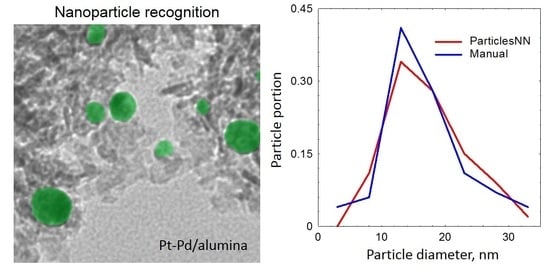
2.2. Comparison with Manual Analysis

For the recognized contours, the area of each particle within the contour and projected area diameter (d = (4S/π)^0.5) are calculated automatically by ParticlesNN.

A typical TEM image of the catalyst Pt-Pd/Al₂O₃ was taken to compare the results of particle size analysis made by ParticlesNN and manually using common ImageJ software [20]. The results of the analysis are shown in Figure 4 and Figure 5 and

Table 4. Processing of TEM image: comparison of ParticlesNN and manual analysis.

Method of Particle Size Determining	Number of Particles	Mean Particle Size, nm	Standard Error Of Mean, nm
Manually	54	17.2	1.8
ParticlesNN	53 *	17.6	1.6

* ‘Face’ particles only.

. It is clear that the mean particle sizes estimated by both methods match each other, with a divergence of ~2%. This is good enough for research. Particle size histograms for both approaches are the same shape. It should be mentioned that ParticlesNN processing time per image is less than 1 min and manual analysis can take hours depending on the user’s experience.

Using manual identification, the operator found 54 particles. Processing by ParticlesNN identified 53 ‘Face’ particles and 7 ‘Bottom’ particles. Two particles were identified as ‘edge particles’, which is optional. In Figure 4b,c, a false positive particle, located at the place of support material thickening, is visible and a set of particles clearly visible by the naked eye was missed by ParticlesNN (Figure 4a). Nevertheless, the set of truth positive particles is representative enough to get an accurate match of mean sizes obtained by ParticlesNN and ImageJ. Missed recognitions due to support material thickening, is a typical data analysis operator error. This can be eliminated, for example, by additional experiments with higher resolution but this is not always possible.

Moreover, in Figure 4b,c, the overlapping of ‘Face’ and ‘Bottom’ particles (blue coloration) is visible. Researchers would recognize this particle as ambiguous for particle size measurement. Labeling the particles with the ‘Bottom’ legend, made by ParticlesNN, is useful to exclude such questionable particles from the statistical analysis. From this point of view, misrecognition of the ‘Bottom’ particle type is preferable since the user can exclude or adjust mistrusted particles during the post-processing stage.

When supported particles are spherical or quasi-spherical shaped, manual size measuring is relatively routine. However, particles can be elongated or present with an arbitrary shape, causing a lot of complications and increasing the analysis time. Figure 6 and

Table 5. Particle size measuring by ParticlesNN and manually.

	Particle Size (pix)
	Particle 1	Particle 2
ParticlesNN, d	74.5	79.8
ImagJ
D1	84.4	94.9
D2	62.9	66.7
Dmean	73.7	80.8
D3	74.2	79.7

show the results of particle size measurement of elongated particles by ParticlesNN and manually. To get the mean particle diameter manually, we need to measure the two main diameters and calculate the mean diameter (Figure 6b) or measure the ‘diagonal’ diameter, which can only be done by experienced researchers. ParticlesNN calculates the diameter precisely based on the number of each particle’s pixels and gives a projected particle diameter (d = (4S/π)^0.5) that can be used for direct statistical analysis. The determined diameter agrees precisely with the results of thorough manual measurement (see Table 5). So, the divergence of the ParticlesNN and manual ImageJ size measurements for individual truth positive contours is less than 1%. The difference of mean particle size between ParticleNN and ImageJ obtained for the whole image originates from false positive and false negative contours. The contribution of FN and FP particles is smoothed by the large number of analyzed particles and the total error stays within 2%.

A comparison of STM and TEM models of particle recognition shows that the accuracy of a particle search is better for STM images (Precision is 0.93, Recall is 0.78 [7]), but particle size determination accuracy is higher for TEM data (2% versus 5%). Particles on TEM images have sharper borders due to a contrast in comparison to STM. At the same time, the variability of artifacts on TEM images causes issues with a TP contour search.

It is important to know that the result of image processing by the ParticlesNN web service is presented not just as a BMP file, where predicted contours are plotted on the original image, but also as a JSON file. Using the LabelMe program the operator can exclude FP, add FN, or adjust TP contours and upload the adjusted file in ParticlesNN for corrected statistics, which decreases the analysis error.

We also compared our service with available software for automatic object detection. Figure 7a shows the result of the application of the “flooding” procedure in the WSxM software [36] for the TEM image in Figure 4a. Particles look like dark spots, so ‘holes’ were chosen for recognition by threshold adjustment. Flooding found 64 objects, the mean projected diameter was 9 nm. Figure 7b shows a histogram of the particle size distribution, which differs significantly from those of Figure 5. It can be easily observed with manual analysis that the increase in particle number and decrease in mean particle size are the result of: (1) false recognition of the dark spots of the support material thickness non-uniformity; (2) distortion of the particle shape/contour due to the particle’s coloring non-uniformity. We obtained similar results by threshold analysis using Digimizer software [37]. For better results, both threshold and min/max length adjustments were used. Mean particle length was 9.0 nm with standard error of 16.7 nm, which is far from manual analysis. So, we conclude that the procedures based on threshold approaches work poorly for TEM images of samples of catalysts on porous supports. Moreover, such procedures do not consider particle projection overlapping.

3. Materials and Methods

3.1. TEM Data

Catalysts consisting of metal nanoparticles (Pt, Pd, etc.) deposited on porous supports of different natures (alumina, silica, titanium dioxide, carbon material ‘Sibunit’) and prepared by the wet impregnation method [1] were used in this work.

The transmission electron microscopy study was performed on a JEM-2010, Jeol Co., Japan, with a lattice resolution of 0.14 nm and an accelerating voltage of 200 kV. The samples of catalysts were fixed on standard copper meshes placed into the holder and put in the chamber of the electron microscope [1]. To determine the particle size, ImageJ software was used [20]. Common for statistical analysis, the selection of no less than 250 measured particles for each sample should be used to obtain mean particle size and to make particle size distribution histograms.

3.2. Dataset

The training dataset and test dataset consist of 31 TEM images with the annotations of 1428 nanoparticles labeled by the operator (ground truth contours (GT)). Dataset images were obtained from original TEM files, which were saved in BMP and JPEG file formats.

Particles were labelled as polygons in the LabelMe program [38] on images colored in a grayscale palette. After being unloaded from LabelMe, JSON files with annotations were converted to COCO format [39], forming files with the annotations of particles.

3.3. Neural Networks

Neural networks in the Cascade Mask-RCNN family [40] were used with a backbone of X-101-64 x4d-FPN. The networks were trained using an MMdetection framework [41] and fine-tuned on our dataset for 500 epochs with a learning rate of 0.005 in epochs 0-332; 0.0005 in 333–457 epochs, and 0.00005 for the subsequent epochs.

3.4. Evaluation

The mean average precision (mAP) [42] with a set of threshold values (0.5, 0.55, 0.6, 0.65, 0.7, 0.75, 0.8, 0.85, 0.9, and 0.95) was used as a quality metric for predicted nanoparticles. In brief, metrics estimate the extent of the union intersection between prediction and ground truth averaged over all classes and the set of threshold values. Values of mAP of 0 (or 0%) correspond to poor predictions while mAP close to 1 (or 100%) signals pixel-to-pixel overlap predictions and the ground truth. mAP metrics were evaluated using a COCO API tool [43] with annotations (annType) of ‘bbox’ type and a maximum particle number (maxDets) of 500.

Training and recognition were carried out on the HPE Apollo 6500 Gen10 graphics server with eight NVIDIA Tesla V-100 graphics accelerators at the Novosibirsk State University Higher College of Informatics.

3.5. Web Service

The TEM image analysis model developed was integrated into the “ParticlesNN” web service (http://particlesnn.nsu.ru, accessed on 12 January 2022) [7] as the Processing ML model “TEM image processing v. 1.1”. For detailed instructions, look for the section “Manual” on the service’s website. TEM images can be uploaded on the website as BMP or JPEG files. The particle recognition result is presented as:

BMP and JSON files with predicted contours;

Tables with results of identification and size measurements for every recognized contour;

Results of statistical analysis (mean particle size, particle size distribution histograms).

The advantages of ParticlesNN as compared to other software products are: (1) It can process images that contain noise and artifacts that are typical for microscopy data without additional processing; (2) The user does not need coding skills. (3) The web service is available to any user, anywhere in the world. (4) The user can adjust automatically determined contours with the help of external software products (for example, LabelMe). (5) Joint statistical processing of the image sets is available. (6) Processing results are displayed in the form of a histogram and tables where information on every identified object is available for users. (7) There is optional consideration of particles at the image boundary for more correct statistical analysis.

4. Conclusions

In this study, we used deep learning for the automatic recognition and size measurements of particles deposited on porous supports on TEM images. The results of the proposed approach were compared with common ‘manual’ TEM data analysis. The error of mean particle size estimation is approximately 2%, which satisfies research tool requirements. The advantages of using deep learning methods for automatic particle recognition were clearly demonstrated:

1. Analysis is faster (compared to manual analysis);

2. Objectivity of measurements (independent of user personality and experience);

3. The neural network takes into account specific features, such as a non-uniform background due to particle projection overlapping or support thickening, etc.

The integration of automatic particle recognition on TEM images in the ParticlesNN web service makes the application of this proposed approach ‘user friendly’ and provides additional tools. For example, the user can automatically adjust determined contours with the help of external software products. This approach to particle recognition using neural networks allows us to improve the quality of recognition over time by accumulating marked data. Integration of the model of TEM image processing into the ParticlesNN web service [7] makes it possible for any user, anywhere in the world to use the results of our work for particle recognition in TEM images.

References

1. Nartova, A.V.; Kovtunova, L.K.; Khudorozhkov, A.K.; Shefer, K.I.; Shterk, G.V.; Kvon, R.I.; Bukhtiyarov, V.I. Influence of preparation conditions on catalytic activity and stability of platinum on alumina catalysts in methane oxidation. Appl. Catal. A Gen. 2018, 566, 174–180. [Google Scholar] [CrossRef]
2. Hansen, T.W.; Delariva, A.T.; Challa, S.R.; Datye, A.K. Sintering of Catalytic Nanoparticles: Particle Migration or Ostwald Ripening? Acc. Chem. Res. 2013, 46, 1720–1730. [Google Scholar] [CrossRef]
3. Akita, T.; Kohyama, M.; Haruta, A. Electron Microscopy Study of Gold Nanoparticles Deposited on Transition Metal Oxides. Acc. Chem. Res. 2013, 46, 1773–1782. [Google Scholar] [CrossRef] [PubMed]
4. Hayden, B.E. Particle Size and Support Effects in Electrocatalysis. Acc. Chem. Res. 2013, 46, 1858–1866. [Google Scholar] [CrossRef] [PubMed]
5. Hutchings, G.J.; Kiely, C.J. Strategies for the Synthesis of Supported Gold Palladium Nanoparticles with Controlled Morphology and Composition. Acc. Chem. Res. 2013, 46, 1759–1772. [Google Scholar] [CrossRef] [PubMed]
6. Lu, J.; Elam, J.W.; Stair, P. Synthesis and Stabilization of Supported Metal Catalysts by Atomic Layer Deposition. Acc. Chem. Res. 2013, 46, 1806–1815. [Google Scholar] [CrossRef]
7. Okunev, A.G.; Mashukov, M.Y.; Nartova, A.V.; Matveev, A.V. Nanoparticle Recognition on Scanning Probe Microscopy Images Using Computer Vision and Deep Learning. Nanomaterials 2020, 10, 1285. [Google Scholar] [CrossRef] [PubMed]
8. Russ, J.C. Computer—Assisted Microscopy: The Measurement and Analysis of Images; Plenum Press: New York, NY, USA, 1990; p. 451. [Google Scholar]
9. Krizhevsky, A.; Sutskever, I.; Hinton, G. Imagenet Classification with Deep Convolutional Neural Networks. In Proceedings of the Annual Conference on Neural Information Processing Systems (NIPS 2012), Lake Tahoe, NV, USA, 3–8 December 2012; pp. 1–9. [Google Scholar]
10. Liu, W.; Anguelov, D.; Erhan, D.; Szegedy, C.; Reed, S.; Fu, C.-Y.; Berg, A.C. SSD: Single Shot MultiboxDetector. In Computer Vision—ECCV 2016; Lecture Notes in Computer, Science; Leibe, B., Matas, J., Sebe, N., Welling, M., Eds.; Springer: Cham, Switzerland, 2016; Volume 9905, pp. 21–37. [Google Scholar]
11. He, K.; Gkioxari, G.; Dollar, P.; Girshick, R. Mask R-CNN. In Proceedings of the 2017 IEEE InternationalConference on Computer Vision (ICCV), Venice, Italy, 22–29 October 2017; pp. 2980–2988. [Google Scholar]
12. Stringer, C.; Michaelos, M.; Pachitariu, M. Cellpose: A generalist algorithm for cellular segmentation. Nat. Methods 2021, 18, 100–106. [Google Scholar] [CrossRef] [PubMed]
13. Moen, E.; Bannon, D.; Kudo, T.; Graf, W.; Covert, M.; Van Valen, D. Deep learning for cellular image analysis. Nat. Methods 2019, 16, 1233–1246. [Google Scholar] [CrossRef] [PubMed]
14. Caicedo, J.; Goodman, A.; Karhohs, K.; Cimini, B.; Ackerman, J.; Haghighi, M.; Heng, C.; Becker, T.; Doan, M.; McQuin, C.; et al. Nucleus segmentation across imaging experiments: The 2018 Data Science Bowl. Nat. Methods 2019, 16, 1247–1253. [Google Scholar] [CrossRef] [PubMed]
15. Yi, J.; Wu, P.; Hoeppner, D.J.; Metaxas, D. Pixel-wise neural cell instance segmentation. In Proceedings of the 2018 IEEE 15th International Symposium on Biomedical Imaging (ISBI 2018), Washington, DC, USA, 4–7 April 2018; pp. 373–377. [Google Scholar]
16. Fu, G.; Sun, P.; Zhu, W.; Yang, J.; Cao, Y.; Ying-Yang, M.; Cao, Y.A. Deep-learning-based approach for fast and robust steel surface defects classification. Opt. Lasers Eng. 2019, 121, 397–405. [Google Scholar] [CrossRef]
17. Poletaev, I.; Tokarev, M.P.; Pervunin, K.S. Bubble Patterns Recognition Using Neural Networks: Application to the Analysis of a Two-phase Bubbly Jet. Int. J. Multiph. Flow 2020, 126, 103194. [Google Scholar] [CrossRef]
18. McQuin, C.; Goodman, A.; Chernyshev, V.; Kamentsky, L.; Cimini, B.; Karhohs, K.; Doan, M.; Ding, L.; Rafelski, S.; Thirstrup, D.; et al. CellProfiler 3.0: Next-generation image processing for biology. PLoS Biol. 2018, 16, e2005970. [Google Scholar] [CrossRef] [PubMed] [Green Version]
19. Berg, S.; Kutra, D.; Kroeger, T.; Straehle, C.; Kausler, B.; Haubold, C.; Schiegg, M.; Ales, J.; Beier, T.; Rudy, M.; et al. ilastik: Interactive machine learning for (bio)image analysis. Nat. Methods 2019, 16, 1226–1232. [Google Scholar] [CrossRef]
20. Schindelin, J.; Arganda-Carreras, I.; Frise, E.; Kaynig, V.; Longair, M.; Pietzsch, T.; Preibisch, S.; Rueden, C.; Saalfeld, S.; Schmid, B.; et al. Fiji: An open-source platform for biological-image analysis. Nat. Methods 2010, 9, 676–682. [Google Scholar] [CrossRef] [Green Version]
21. Bannon, D.; Moen, E.; Schwartz, M.; Borba, E.; Kudo, T.; Greenwald, N.; Vijayakumar, V.; Chang, B.; Pao, E.; Osterman, E.; et al. DeepCell Kiosk: Scaling deep learning–enabled cellular image analysis with Kubernetes. Nat. Methods 2021, 18, 43–45. [Google Scholar] [CrossRef] [PubMed]
22. Okunev, A.G.; Nartova, A.V.; Matveev, A.V. Recognition of Nanoparticles on Scanning Probe Microscopy Images Using Computer Vision and Deep Machine Learning. In Proceedings of the International Multi-Conference on Engineering, Computer and Information Sciences (SIBIRCON), Novosibirsk, Russia, 21–27 October 2019; pp. 940–943. [Google Scholar]
23. Zhu, H.; Ge, W.; Liu, Z. Deep Learning-Based Classification of Weld Surface Defects. Appl. Sci. 2019, 9, 3312. [Google Scholar] [CrossRef] [Green Version]
24. Liu, Y.; Xu, K.; Xu, J. Periodic Surface Defect Detection in Steel Plates Based on Deep Learning. Appl. Sci. 2019, 9, 3127. [Google Scholar] [CrossRef] [Green Version]
25. Feng, S.; Zhou, H.; Dong, H. Using Deep Neural Network with Small Dataset to Predict Material Defects. Mater. Des. 2019, 162, 300–310. [Google Scholar] [CrossRef]
26. Yang, T.; Xiao, L.; Gong, B.; Huang, L. Surface Defect Recognition of Varistor Based on Deep Convolutional Neural Networks. In Optoelectronic Imaging and Multimedia Technology VI, Proceedings of the SPIE/COS PHOTONICS ASIA, Hangzhou, China, 20–23 October 2019; Dai, Q., Shimura, T., Zheng, Z., Eds.; International Society for Optics and Photonics: Bellingham, WA, USA, 2019; Volume 11187, p. 1118718. [Google Scholar]
27. Ziatdinov, M.; Dyck, O.; Maksov, A.; Li, X.; Sang, X.; Xiao, K.; Unocic, R.; Vasudevan, R.; Jesse, S.; Kalinin, S.V. Deep Learning of Atomically Resolved Scanning Transmission Electron Microscopy Images: Chemical Identification and Tracking Local Transformations. ACS Nano 2017, 11, 12742–12752. [Google Scholar] [CrossRef] [Green Version]
28. Modarres, M.H.; Aversa, R.; Cozzini, S.; Ciancio, R.; Leto, A.; Brandino, G.P. Neural Network for Nanoscience Scanning Electron Microscope Image Recognition. Sci. Rep. 2017, 7, 13282. [Google Scholar] [CrossRef] [Green Version]
29. Qu, E.Z.; Jimenez, A.M.; Kumar, S.K.; Zhang, K. Quantifying Nanoparticle Assembly States in a Polymer Matrix Through Deep Learning. Macromolecules 2021, 54, 3034–3040. [Google Scholar] [CrossRef]
30. Monchot, P.; Coquelin, L.; Guerroudj, K.; Feltin, N.; Delvallée, A.; Crouzier, L.; Fischer, N. Deep Learning Based Instance Segmentation of TitaniumDioxide Particles in the Form of Agglomerates in ScanningElectron Microscopy. Nanomaterials 2021, 11, 968. [Google Scholar] [CrossRef] [PubMed]
31. Qian, Y.; Huang, J.Z.; Li, X.; Ding, Y. Robust Nanoparticles Detection from Noisy Background by Fusing Complementary Image Information. IEEE Trans. Image Process. 2016, 25, 5713–5726. [Google Scholar] [CrossRef] [PubMed]
32. Park, C.; Ding, Y. Automating material image analysis for material discovery. MRS Commun. 2019, 9, 545–555. [Google Scholar] [CrossRef] [Green Version]
33. Wei, Y.; Chen, H.; Wang, H.; Wei, D.; Wu, Y.; Fan, K. Detection of Nano-particles Based on Machine Vision. In Proceedings of the 2019 IEEE International Conference on Manipulation, Manufacturing and Measurement on the Nanoscale (3M-NANO), Zhenjiang, China, 4–8 August 2019; pp. 189–192. [Google Scholar]
34. Oktay, A.B.; Gurses, A. Automatic detection, localization and segmentation of nano-particles with deep learning in microscopy images. Micron 2019, 120, 113–119. [Google Scholar] [CrossRef]
35. Zhang, F.; Zhang, Q.; Xiao, Z.; Wu, J.; Liu, Y. Spherical Nanoparticle Parameter Measurement Method based on Mask R-CNN Segmentation and Edge Fitting. In Proceedings of the 8th International Conference on Computing and Pattern Recognition (ICCPR’19), Beijing, China, 23–25 October 2019; pp. 205–212. [Google Scholar]
36. Horcas, I.; Fernandez, R.; Gomez-Rodriguez, J.M.; Colchero, J.; Gomez-Herrero, J.; Baro, A.M. WSXM: A Software for Scanning Probe Microscopy and a Tool for Nanotechnology. Rev. Sci. Instrum. 2007, 78, 013705. [Google Scholar] [CrossRef]
37. Schoonjans, F. Digimizer Manual: Easy-to-Use Image Analysis Software; 2019; 107p, ISBN 9781706417149. [Google Scholar]
38. Wada, K. Labelme: Image Polygonal Annotation with Python. 2016. Available online: https://github.com/wkentaro/labelme (accessed on 1 June 2020).
39. Lin, T.-Y.; Maire, M.; Belongie, S.; Bourdev, L.; Girshick, R.; Hays, J.; Perona, P.; Ramanan, D.; Zitnick, C.L.; Dollár, P. Microsoft COCO: Common Objects in Context. Lect. Notes Comput. Sci. 2014, 8693, 740–755. [Google Scholar]
40. Cai, Z.; Vasconcelos, N. Cascade R-CNN: Delving into High Quality Object Detection. In Proceedings of the IEEE Conference on Computer Vision and Pattern Recognition (CVPR), Salt Lake City, UT, USA, 18–22 June 2018; pp. 6154–6162. [Google Scholar]
41. Chen, K.; Wang, J.; Pang, J.; Cao, Y.; Xiong, Y.; Li, X.; Sun, S.; Feng, W.; Liu, Z.; Xu, J.; et al. MMDetection: Open MMLab Detection Toolbox and Benchmark. arXiv 2019, arXiv:1906.07155. [Google Scholar]
42. Everingham, M.; Van Gool, L.; Williams, C.K.I.; Winn, J.; Zisserman, A. The Pascal Visual Object Classes (voc) Challenge. Int. J. Comput. Vis. 2010, 88, 303–338. [Google Scholar] [CrossRef] [Green Version]
43. COCO API—Dataset. Available online: https://github.com/cocodataset/cocoapi (accessed on 1 June 2020).
Figure 1. Typical TEM image of the support catalyst (Pt nanoparticles on carbon support ‘Sibunit’).
Catalysts 12 00135 g001
Figure 2. TEM images of Pt on alumina catalyst with ground truth contours: (a) individual ‘Face’ particles; (b) overlapping but visible ‘Face’ particles; (c) overlapping ‘Bottom’ particles with poorly visible borders.
Catalysts 12 00135 g002
Figure 3. TEM image of Pt on alumina catalyst from test dataset with 19 ‘Face’ TP (red), 3 ‘Bottom’ TP (green), 5 ‘Bottom’ FN (blue).
Catalysts 12 00135 g003
Figure 4. Result of particle recognition of TEM image of Pt-Pd on alumina catalyst processed by ParticlesNN (a) (‘Face’ particles are of green coloration; ‘Bottom’ are of blue coloration; pink coloration for ‘edge particle’): crops of processed image (b) and original image (c).
Catalysts 12 00135 g004
Figure 5. Particle size histograms: ParticlesNN (a) and manual analysis (b).
Catalysts 12 00135 g005
Figure 6. Result of particle recognition of TEM image processed by ParticlesNN (a) and manual size measuring by ImageJ (b).
Catalysts 12 00135 g006
Figure 7. Processing of the TEM image (Figure 4a) by the “flooding” procedure in WSxM software (a); particle size distributions of the defined 64 contours (b).
Catalysts 12 00135 g007