Enhancing the Predictive Modeling of n-Value Surfaces in Various High Temperature Superconducting Materials Using a Feed-Forward Deep Neural Network Technique

Abstract

In this study, the prediction of n-value (index-value) surfaces—a key indicator of the field and temperature dependence of critical current density in superconductors—across various high-temperature superconducting materials is addressed using a deep learning modeling approach. As superconductors play a crucial role in advanced technological applications in aerospace and fusion energy sectors, improving their performance model is essential for both practical and academic research purposes. The feed-forward deep learning network technique is employed for the predictive modeling of n-value surfaces, utilizing a comprehensive dataset that includes experimental data on material properties and operational conditions affecting superconductors’ behavior. The model demonstrates enhanced accuracy in predicting n-value surfaces when compared to traditional regression methods by a 99.62% goodness of fit to the experimental data for unseen data points. In this paper, we have demonstrated both the interpolation and extrapolation capabilities of our proposed DFFNN technique. This research advances intelligent modeling in the field of superconductivity and provides a foundation for further exploration into deep learning predictive models for different superconducting devices.

1. Introduction

Superconducting materials hold significant importance in existing technological and scientific fields—including aviation, defense, medical, and energy sectors—due to their unique ability to conduct electrical current without resistance in direct current mode when cooled below a certain critical temperature [1,2,3,4,5]. In addition to the sensitivity of superconductors to operating temperature, these materials have a physical limitation in terms of their current flow [6]. Critical current—usually reported in the form of critical current density—is a fundamental property of superconducting materials, representing the maximum current they can carry without losing their superconducting state [7,8]. Beyond this threshold, the material experiences a transition to a normal resistive state [9,10]. The n-value, on the other hand, describes the sharpness of the transition from the superconducting state to the normal resistive state as the current density approaches the critical current density and is a sample-specific phenomenon that its pattern varies in different High Temperature Superconductor (HTS) samples and under different operating temperatures [11]. Normally, the n-value can be evaluated from the power-law formula, which is shown in Equation (1). In this equation, $E$ is the electric field, $E_c$ is the field when critical current flows through the sample, $J$ is the current density, $J_c$ is the critical current density, B is the magnetic field, $\theta$ is the magnetic field angle with respect to the superconductor surface, and T is the operating temperature [12,13].

$$\frac{E}{E_c}={\left(\frac{J}{J_c(B,T,\theta )}\right)}^{n\left(B,T,\theta \right)}$$

(1)

Generally, high n-values indicate a sharp transition, which is desirable for maintaining stability in superconducting applications, especially for high-precision applications like MRI machines and particle accelerators [11,14]. The n-value surfaces refer to the graphical representation of n-values over a range of operating conditions, such as temperature and magnetic field strength [15,16]. These highly non-linear surfaces provide a comprehensive understanding of the material’s performance and stability across different working conditions, which highlights their importance for optimizing the use of superconductors in various applications [17,18]. Therefore, the accurate prediction of n-value helps model superconductors’ behavior more accurately, design more efficient superconducting devices, enhance performance, and reduce operational risks [19].

Traditionally, estimating the n-value has relied on look-up tables and empirical methods, which are limited by their dependency on pre-existing data and lack of adaptability to new conditions [20]. Moreover, look-up tables rely on linear regression between two available data points, which will increase the error of estimation as the changing pattern of the n-value is extremely non-linear. However, in recent years, artificial intelligence (AI) techniques have been proposed and employed—despite being overlooked for many decades—for many applications in superconductivity, including for the intelligent modeling of superconductors [21,22,23,24]. Simpler machine learning (ML) techniques have improved the estimation process by identifying patterns of the n-value, providing more accurate predictions in significantly less time than even look-up tables [20,25].

In most of the works that have focused on the estimation of the n-value by ML methods, the models were developed to accurately estimate only one sample of superconductors [20,25], and in [26], the authors considered three superconductor samples. This study aims to advance toward developing more general solutions that can cover several types of superconductors that are commercially available in the market with a deep learning approach, which potentially can handle bigger datasets with extremely high accuracy. This means that the dataset that is going to be used for this work will be way larger than the datasets that have been used by other researchers in the literature.

Deep learning (DL), on the other hand, offers significant advantages by handling vast and complex datasets, capturing intricate patterns, and providing more accurate predictions [27]. The use of deep learning, particularly deep feed-forward neural networks (DFFNNs), in predicting n-value surfaces for HTS materials is motivated by the need for higher accuracy and adaptability [28]. DL models excel in processing large datasets with multiple variables, learning from the data to identify non-linear relationships and subtle dependencies [29]. The availability of massive datasets in superconductivity research enables the training of DL models to a high degree of accuracy [30]. These models generalize well across different conditions, providing reliable predictions even in scenarios not explicitly covered in the training data. By using a DL approach, this study aims to enhance the predictive modeling of n-value surfaces. In fact, this is the main motivation of our paper to use intelligent algorithms to identify this complex pattern by using deep learning approaches to significantly reduce the uncertainty and error of the prediction. This intelligent algorithm is even able to take the outlier points (noisy points that are existing in the dataset due to errors in the experiments) out of consideration and capture the real pattern that the data follow. In this paper, we have demonstrated both the interpolation and extrapolation capabilities of our proposed DFFNN technique, which essentially means that the DFFNN-based model can be effectively used to predict the n-values out of the training range of our intelligent model.

Our innovative model will be able to predict the n-value of multiple superconducting samples with extremely high accuracy and in only milliseconds of time. Therefore, there is no need to utilize different models for individual samples anymore.

2. Materials and Methods

During this section, first, the dataset that is used for this work will be introduced. Then, the architecture of the DL method that is used in this work is proposed. Finally, the metrics that are used for the evaluation and comparison of the performance of the network will be explained.

2.1. Data Collection

Every ML model needs to be trained by a source of data, which can be in the form of a table or image. To provide this dataset, we have collected the data of six HTS conductors including Shanghai Creative Superconductor Technologies SCST-W12 2G HTS, Shanghai Superconductor Low Field High Temperature 2G HTS, Faraday Factory Japan YBCO 2G HTS, Ceraco M-Type YBCO 2G HTS film on sapphire, SuperOx YBCO 2G HTS, and SuperOx GdBCO 2G HTS from an open-access website by Robinson Research Institute (Victoria University of Wellington, Wellington, New Zealand) [31,32]. However, the raw dataset, containing more than 120,000 data points, is not suitable for implementation in an AI algorithm and needs to be pre-processed. To do so, first, the temperature and magnetic field intensity ranges that contain a reasonable number of missing data points must be removed completely. This will ensure that the quality and consistency of the dataset will not be affected by incomplete data which can lead to inaccurate estimates and predictions. After doing so, the dataset size decreases to 92,003 points, covering the n-value of different HTS tapes for a range of temperatures between 15 and 90 K, magnetic field intensity between 0.01 and 8T, and the angle of the magnetic field between 2° and 240°.

Next, the data need to be normalized to a standard scale between 0 and 1 to bring all features onto a similar scale. This is because many machine learning algorithms, particularly those based on gradient descent like the DFFNN, perform better when features are on a similar scale. Normalization helps the algorithm converge faster by preventing features with larger ranges from dominating the updates. Moreover, normalization may lead to more efficient computations. When features are normalized, the optimization landscape becomes smoother, allowing the algorithm to make more consistent progress in each iteration. This can reduce the overall computational time required for training.

Finally, the dataset has to be randomly split into three individual sets for training, validating, and testing purposes, each consisting of 70%, 15%, and 15% of the data, respectively. This is because we ensure that the model is trained with a reasonable amount of data to capture the pattern of the n-value, and the performance of the developed model is tested by using data points that have never been seen by the model before. By comparing the estimated value of the model and the actual values of the experimental data, we can assess how accurately the model performs.

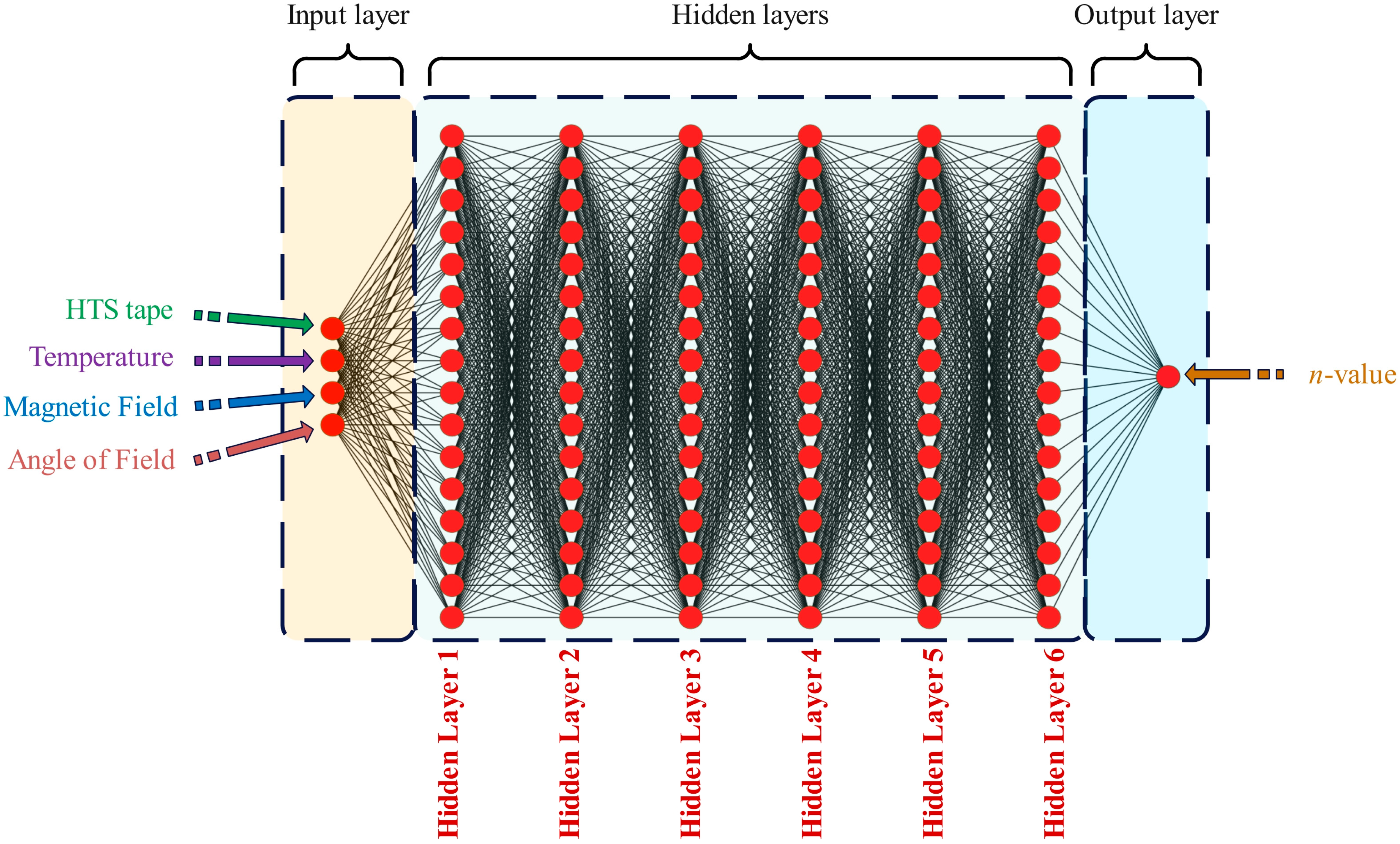
2.2. Architecture of Deep Feed-Forward Neural Network

Deep feed-forward neural networks consist of multiple layers of neurons, each connected to the next in a forward direction, from input to output, without any cycles or loops [33]. The architecture is designed to model complex functions by learning from data through a process of optimization [34,35]. At its core, a deep feed-forward neural network comprises three primary types of layers: the input layer, hidden layers, and the output layer. Each layer consists of nodes or neurons, which are the basic computational units of the network (see Figure 1). In a DFFNN, each connection between neurons is associated with a weight, which adjusts during the training process to minimize the error in the network’s predictions. Each neuron (except those in the input layer) also has an associated bias, which shifts the activation function to help the network learn the data more effectively [36,37,38].

The input layer is the first layer in the network and is responsible for receiving the raw data [39]. Each neuron in the input layer represents a feature or dimension of the input data including a superconductor sample, temperature, magnetic field intensity, and field angle relative to the tape. This has been illustrated in Figure 1. In fact, this layer passes the input values to the subsequent layers without performing any computations [10,40]. This means that these neurons do not have any weight or bias factors to change the values and they only contain the exact input values of each parameter that were mentioned above.

Hidden layers are the intermediate layers between the input and output layers. These layers perform the core computations and transformations on the data [41]. A deep feed-forward neural network has multiple hidden layers, and the term “deep” refers to the presence of these multiple layers [42], making it different from simple FFNN models. Each neuron in a hidden layer receives input from all neurons in the previous layer, processes it through a weighted sum followed by a non-linear activation function, and then passes the output to the neurons in the next layer [43]. The activation function is crucial as it introduces non-linearity into the network and enables it to learn and model complex relationships in the data. Common activation functions include the sigmoid function, hyperbolic tangent (tanh), and the Rectified Linear Unit (ReLU). In this work, we will use tanh and ReLU activation functions for our model, which will be discussed further in Section 3.

The output layer is the final layer of the network, where the results of the computations are produced [44]. The structure and number of neurons in the output layer depend on the specific task. Specifically, for this paper, which focuses on regression tasks, the output layer must consist of a single neuron with a linear activation function to produce continuous values. This neuron will directly estimate the n-value of different superconductors.

2.3. Performance Metrics

In this study, the performance of our DL model is evaluated using several key metrics: R-squared, Root Mean Squared Error (RMSE), mean absolute error (MAE), and Mean Absolute Relative Error (MARE). These metrics provide a comprehensive assessment of the DL model’s accuracy in predicting the target variable.

R-squared, also known as the coefficient of determination, indicates the proportion of the variance in the dependent variable that is predictable from the independent variables. R-squared values range from 0 to 1, with higher values indicating a better fit of the model to the data. An R-squared value close to 1 suggests that a large proportion of the variance in the target variable is explained by the model. The mathematical form of the R-squared can be written as follows:

$$R^2=1-\frac{\sum _{k=1}^K{\left(q_k-y_k\right)}^2}{{\sum _{k=1}^K\left(q_k-\overline{p}\right)}^2}$$

(2)

where $y_k$ is the estimated value, $\overline{y}$ is the mean value of $y$, $n_s$ is the number of samples of the training dataset, $q_k$ are the actual values, and $\overline{q_k}$ is the mean value of $q_k$.

RMSE is a measure of how spread out these residuals are. In essence, RMSE provides a sense of how far the predicted values deviate from the actual values. Lower RMSE values indicate a better fit of the model to the data. RMSE is particularly useful for comparing different models or the same model on different datasets, as it is in the same units as the target variable.

$$RMSE={\left[\frac{1}{K}\sum _{k=1}^K{\left(q_k-y_k\right)}^2\right]}^{\frac{1}{2}}$$

(3)

MAE is the average of the absolute errors between the predicted and actual values. It provides a straightforward measure of the average magnitude of the errors in a set of predictions, without considering their direction. MAE is an intuitive metric that is easy to interpret, with lower values indicating better predictive accuracy.

$$MAE=\sum _{k=1}^K\frac{\left|q_k-y_k\right|}{K}$$

(4)

MRE measures the absolute differences between the predicted and actual values, divided by the actual values, expressed as a percentage. This metric provides insight into the average relative error, making it useful for comparing performance across datasets with different scales. Lower MRE values indicate more accurate predictions relative to the actual values.

$$MRE=100\times \sum _{k=1}^K\frac{q_k-y_k}{y_k\ast K}$$

(5)

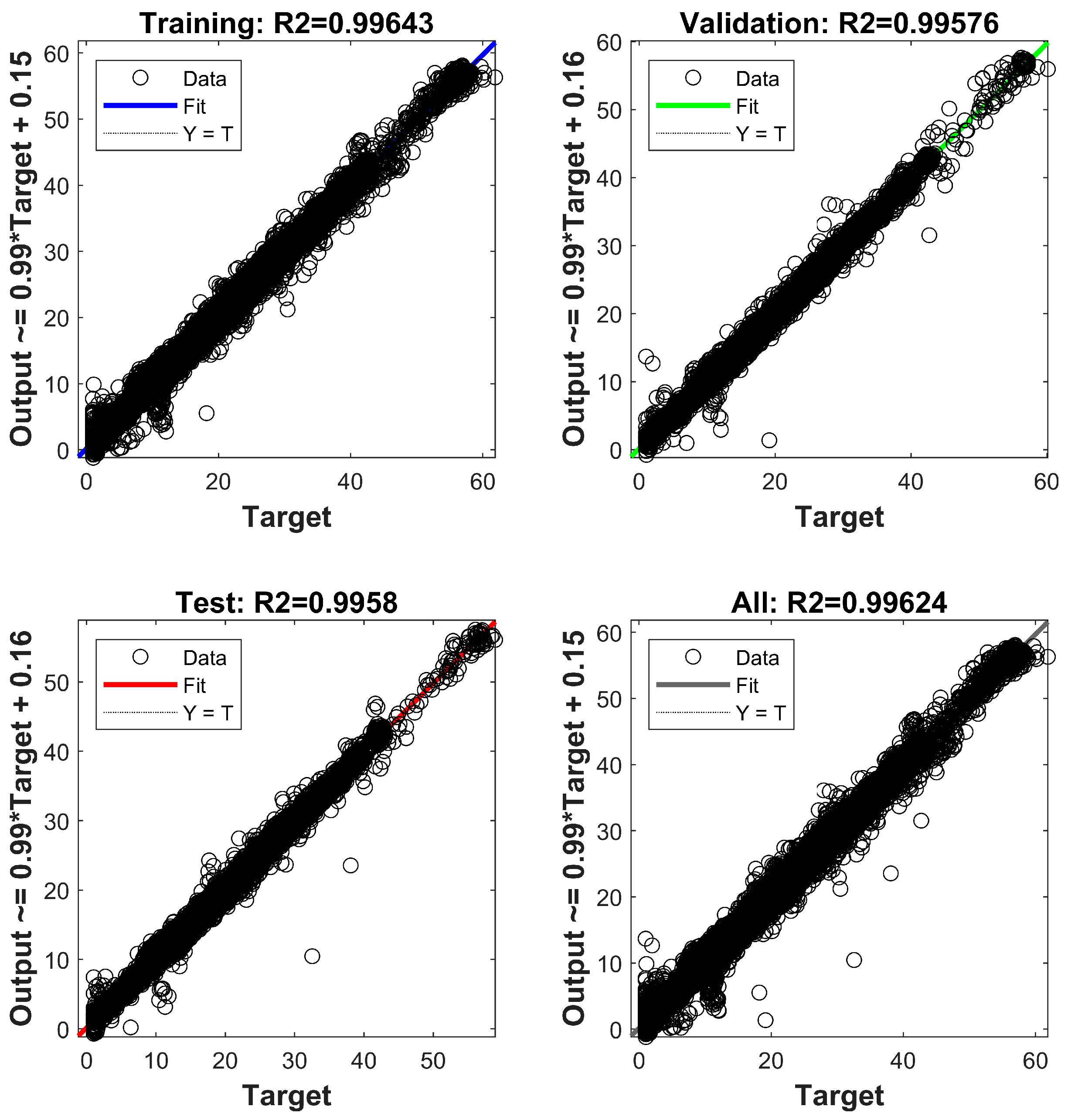
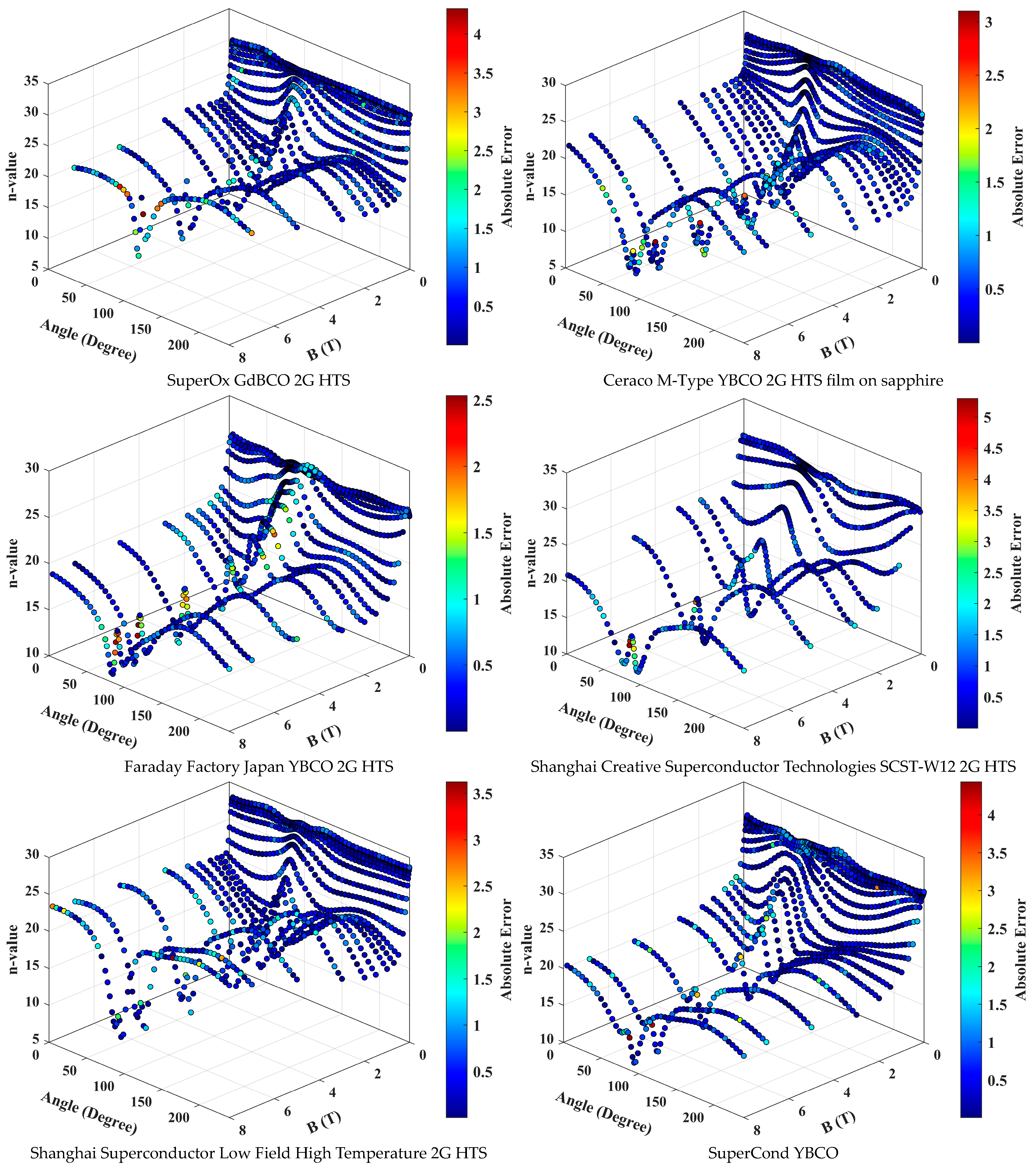
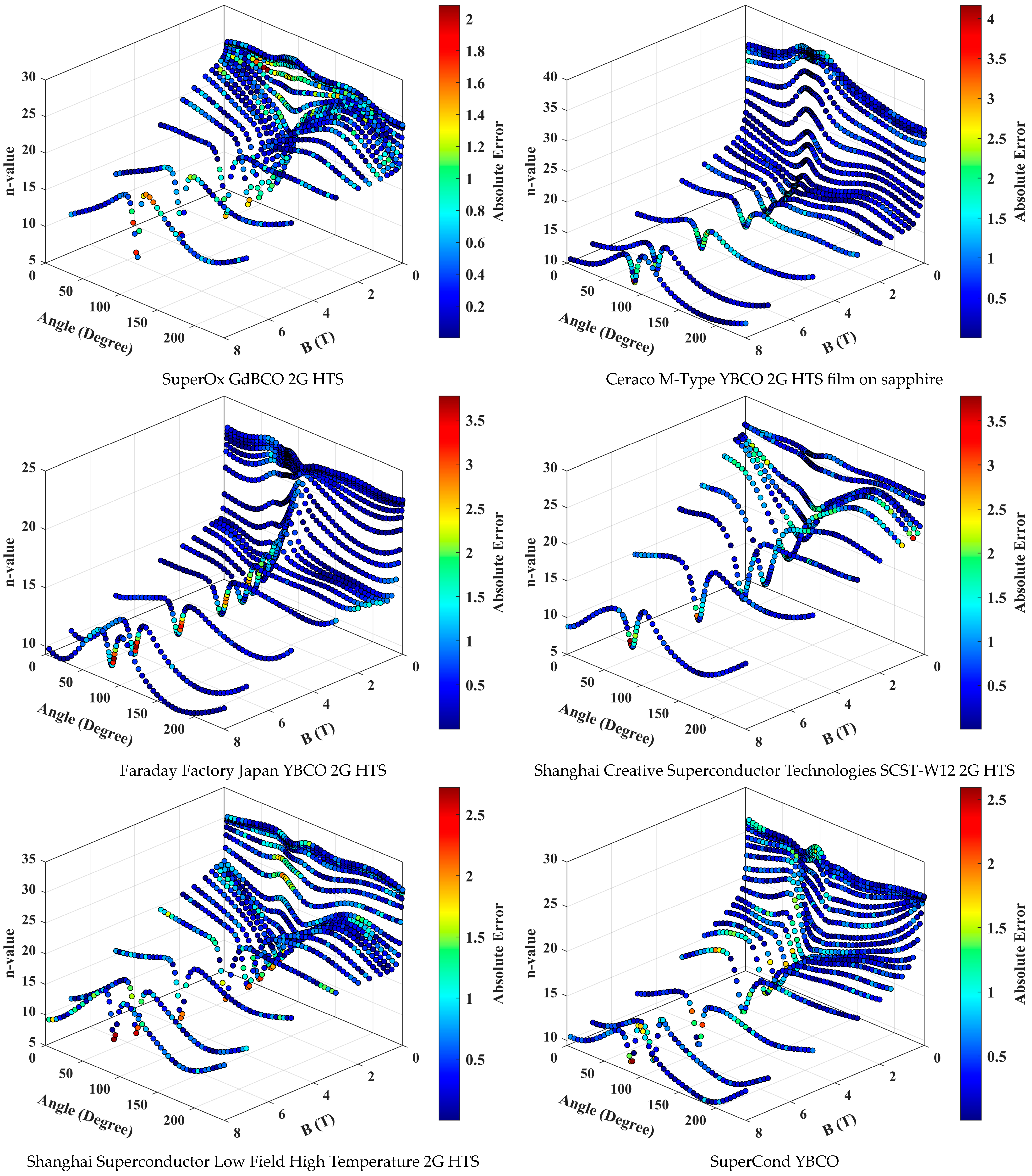
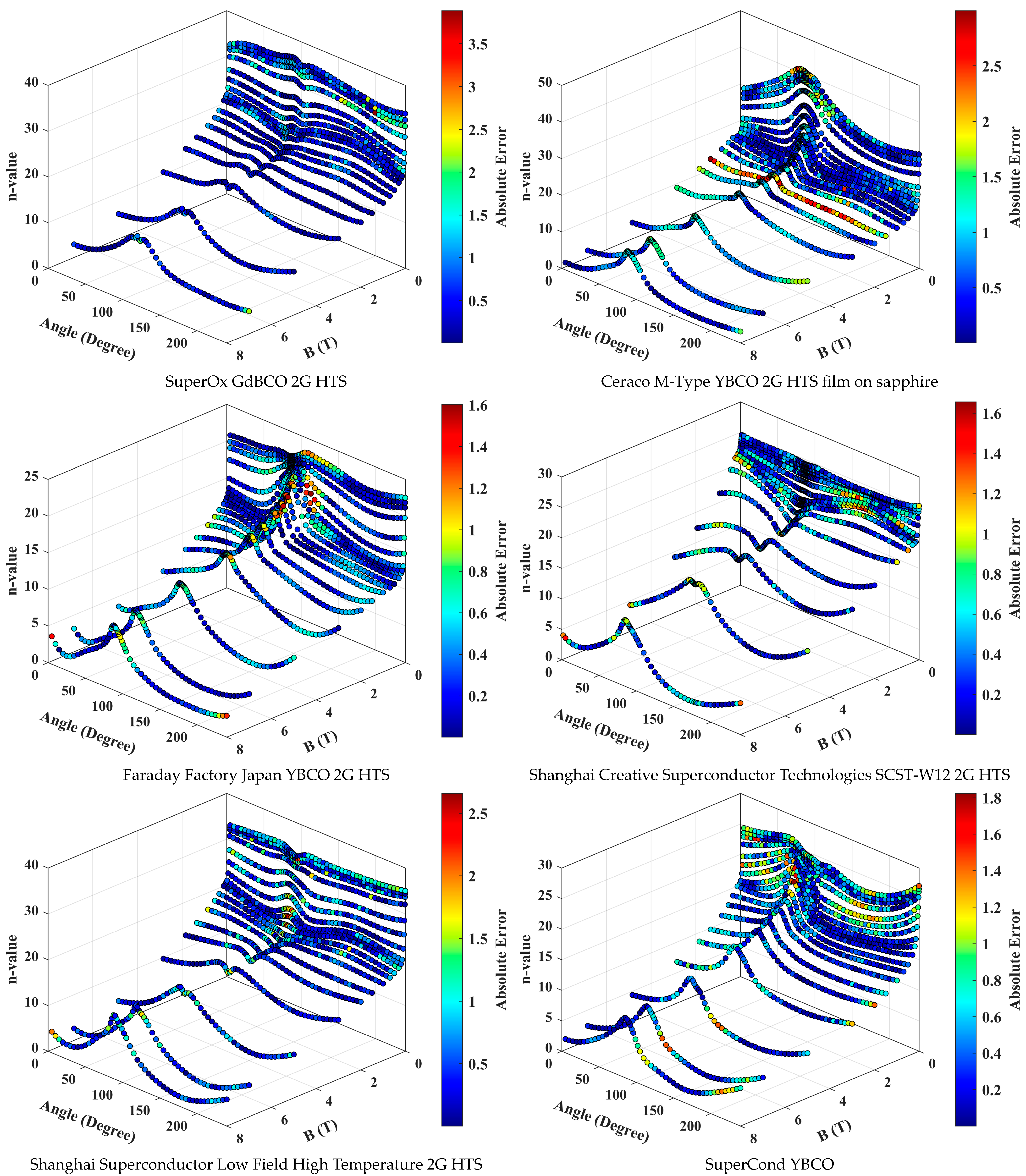
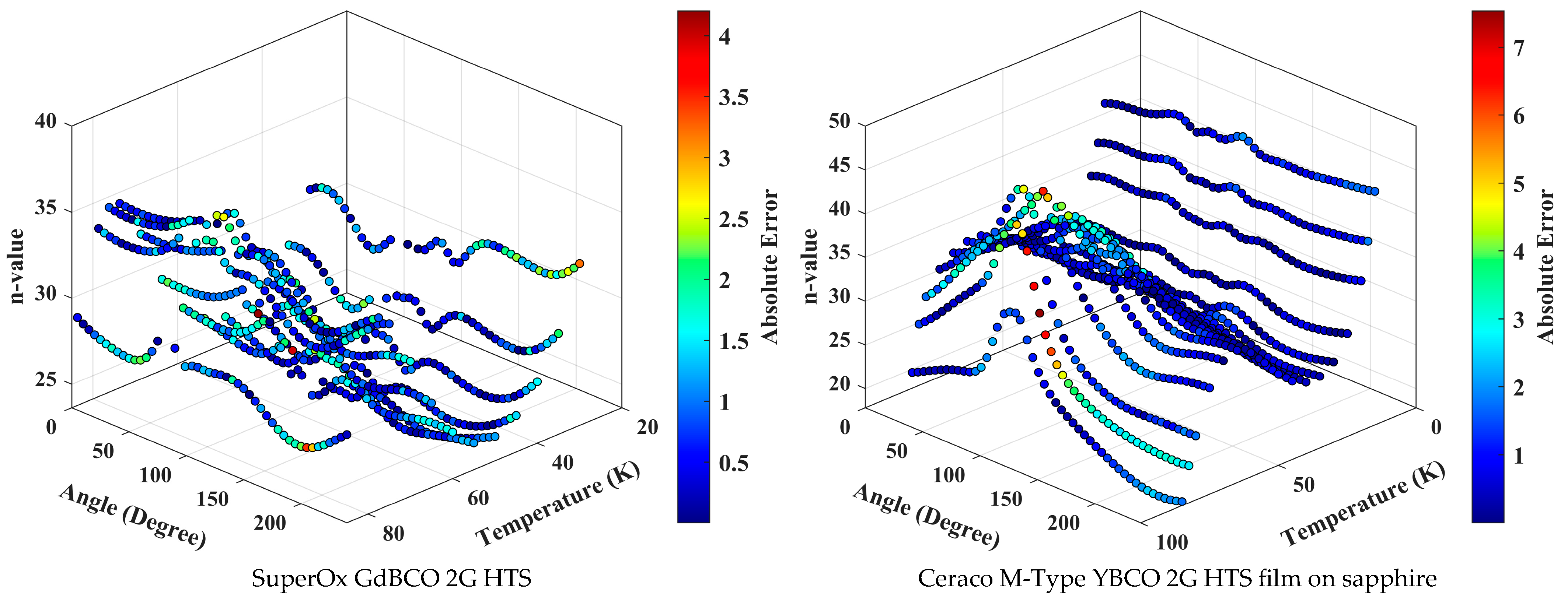
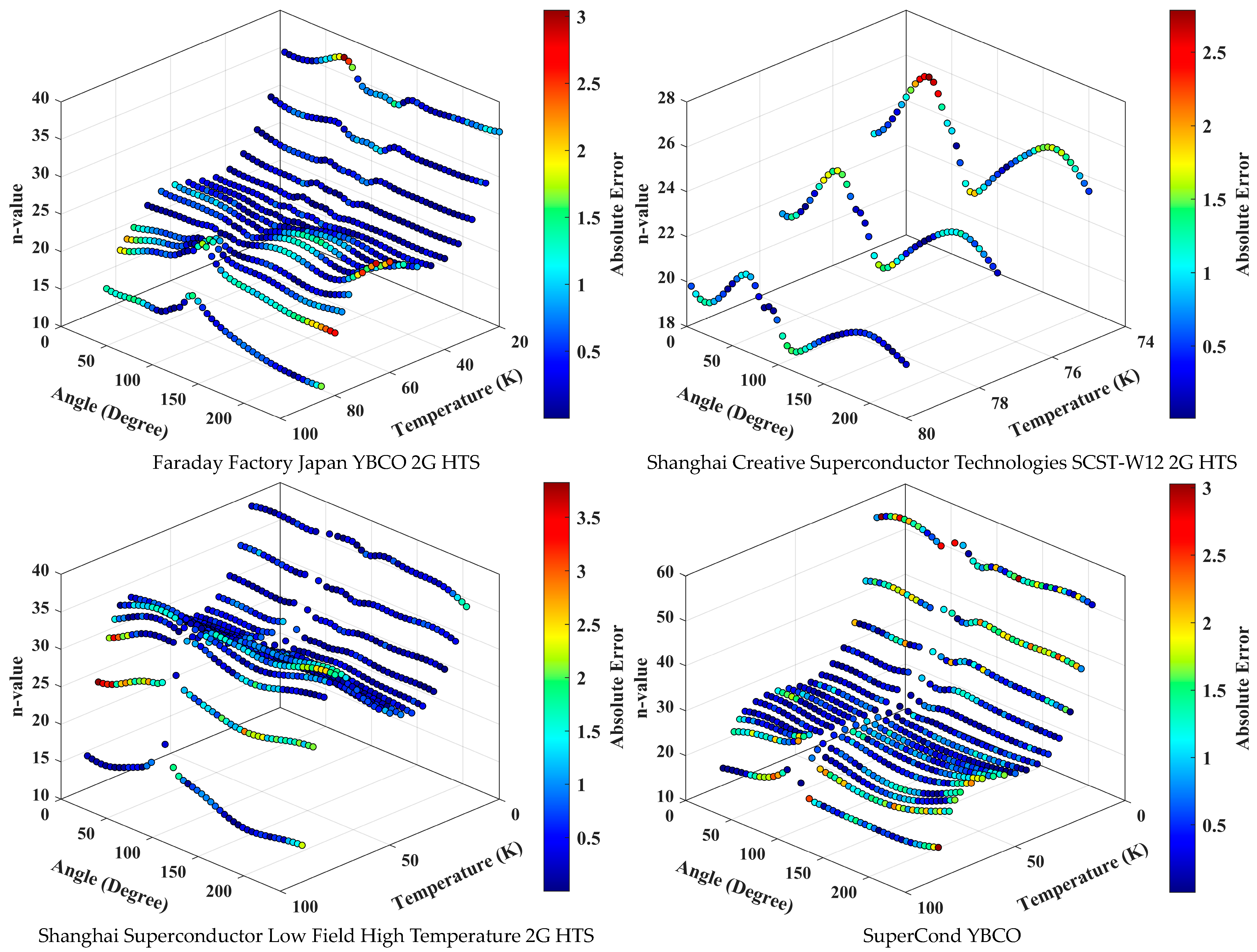
3. Results and Discussion

Now, the data that were prepared in Section 2.1 must be implemented in the algorithm of the DFFNN being explained in Section 2.2. As was described in Section 2.2, there are some effective parameters in the algorithm like the number of hidden layers, the number of neurons in each layer, the activation function, and the optimization algorithm (also known as the training function). After some trial processes and sensitivity analyses on the effects of the number of hidden layers, we have considered six hidden layers for the DFFNN model, with each layer containing 64 neurons as the best structure. Therefore, by considering four neurons of the input layer (equal to the number of input features including the label of sample, temperature, magnitude of the field, and angle of the field), the whole network will have 25,154 free parameters to capture the pattern of the n-value of different superconducting samples. Free parameters are the weights and biases that the network learns during training [45]. We also have considered the “tansig” activation function between the input layer and the hidden layers and between every two hidden layers. This is because the tansig function has an output between −1 and 1 which helps the network’s convergence during the training process by mitigating the vanishing gradient problem. Also, for the activation function between the hidden layer and output layer, the ReLU function has been considered to return the output of the network to the last layer without any scaling. In terms of optimization function, we have considered the Levenberg–Marquardt algorithm to optimize the weight and bias factors of the neurons to minimize the loss of the network. While this optimizer makes the training time of the network longer than other functions and requires more memory on the PC, it has shown accuracy superiority over other conventional functions that are commonly used by researchers.

To train the model, first, an initial and random set of numbers is considered for the weight and bias factors of each neuron. Then, the training data will be introduced to the network and the optimizer function updates the weight and bias factors accordingly to decrease the error from the initial value. This process will be repeated in a loop until the accuracy of the network meets the predefined criteria or the network’s training line starts to diverge. These cycles are known as epochs. This demonstrates that the best validation performance is 0.55622 in terms of MSE (0.7458 in terms of RMSE).

Figure 2 indicates how well the proposed model can estimate the n-value for different materials in terms of R-squared. The evaluation is shown through scatter plots comparing the model outputs to the target values across different datasets: training, validation, testing, and all data. As was discussed before, higher values of R-squared mean the model has a better performance. As it appears from this figure, the developed DFFNN model can predict the n-value with an extremely high accuracy of 99.624% in terms of $R^2.$

As was described in Section 2.1, the method that is used for splitting the dataset into three sets is random, which is a very common method for this step of data pre-processing, used by many AI researchers. The rationale behind choosing this method is to ensure that the training and testing sets are representative of the overall data distribution. This helps in obtaining an unbiased estimate of the model’s performance. This random splitting affects the performance of the model as the training, validating, and testing sets will be different. To overcome this issue, there is a well-known technique, namely ‘data cross-validation’, which ensures that all datapoints are utilized for training and testing. A robust approach of cross-validation is the k-fold method. This technique involves dividing the dataset into k equally sized folds or subsets. Then, the model is trained with k−1 parts of the initial data and tested with the remaining fold. This process is repeated k times while each fold is used one time as the testing dataset. The results of the k-fold cross-validation are as follows:

As can be seen with

Table 1. Performance of DFFNN models using different folds of dataset as testing data.

Number of Fold(s)	R-Squared	RMSE
1	0.99521	0.82374
2	0.99496	0.85219
3	0.99516	0.81372
Mean	0.99511	0.82988

, by considering fold 1 as the testing data and training of the model with the remaining data, the model achieves an R-squared value of 0.99521, indicating a goodness of fit of 0.99521 with the actual experimental values. The RMSE for this fold is 0.82374, showing the squared average error of the predictions from the actual values. For fold 2, the performance of the model relatively decreases as the R-squared value is slightly lower at 0.99496 and RMSE is slightly higher at 0.85219. Finally, for the third fold, the model performance relatively improves again, with an R-squared value of 0.99516, explaining 99.516% of the variance, and an RMSE of 0.81372, which is the lowest among the three folds. These results show that the robust model that has been proposed is not very sensitive to the random selection of the data, as the deviation of R-squared is below 0.0003. This ensures that the proposed model does not perform well only on a specific subset of data but demonstrates its generalizability across the entire dataset.

Once the training process of the model is finished, we test the prediction performance of the model by integrating the sample label, temperature, magnitude of field, and angle of field as inputs to the model and then compare its predicted n-value with experimental ones. For the consistency of the work and to aid better visualization, we have plotted the n-value pattern of different materials for a common temperature.

Figure 3 illustrates the pattern of the n-value with respect to the changes in field magnitude and angle for six different superconducting materials at 30 K. The color of the data points also shows the error between the predicted value and actual value. As can be seen, in most of the data points, the model has an error near to zero. Also, it is evident that for most of the field intensities, the model struggles to accurately predict the n-value for the angles near 90°. This was previously discussed in [20,25] and is due to the topology of the data, as the sharpness of the pattern of n-value is very high and the data are scarce in this region. So, the model is not able to perfectly capture the real pattern near this zone.

Figure 4 and Figure 5 provide the same information, with the difference in the temperature being 60 and 75 K, respectively. These figures show that the DFFNN model effectively captures the non-linear relationships between the variables, providing reliable predictions even under conditions not explicitly covered in the training data.

Table 2. Estimation accuracy of the proposed DFFNN model.

RMSE	R-Squared	MAE	MRE [%]	Testing Time [s]
0.744591657	0.996244289	0.492103476	3.328049383	0.6135193

summarizes the performance of the proposed DFFNN model in terms of all metrics that were discussed in Section 2.3.

It should be highlighted that the testing time of the developed model is the time that the model needs to predict over 13,800 data points. Also, it completely depends on the computational resources that the model is tested on. For this work, we have used a PC with 11th Gen Intel(R) Core(TM) [email protected] GHz CPU and 8.00 GB of RAM with solid-state drive storage.

Moreover, these AI methods are not only beneficial for estimating the points within the training range, but also, they are useful for even out-of-range data, where extrapolation is necessary. To demonstrate that ability of our DFFNN model, we have taken out all datapoints of the initial data which have a field of 0.01 T and used these data for the training of our model. Then, we have used the removed data for testing of the model. This way, we will ensure that our test points (containing 3750 datapoints) are out of the training range of data and the model needs to extrapolate them in order to estimate the n-value. The results of our test (see

Table 3. Estimation accuracy of the proposed DFFNN model for out-of-range data (0.01 T).

RMSE	R-Squared	MAE	MRE [%]	Testing Time [s]
1.058721	0.973809126	0.76842511	2.7668185	0.259087

) demonstrate that the performance of our proposed DFFNN model for predicting is 97.3809% in terms of R-squared and has a MARE of only 2.7668%. The RMSE of this test is also 1.0587. The results of this test demonstrate that AI models can potentially be used for a range of data that has not been trained before. The more detailed prediction ability of this model is presented in Figure 6, where the pattern of n-value has been shown with respect to temperature and field angle changes for a common 0.01 T field.

4. Conclusions

This study demonstrates the significant potential of deep feed-forward neural network (DFFNN) in predicting n-value surfaces for various high-temperature superconducting (HTS) materials. By leveraging a comprehensive dataset encompassing diverse material properties and operational conditions, the DFFNN model developed in this research achieved superior accuracy compared to traditional regression methods. The model’s high precision in estimating n-values across different HTS samples underscores its utility in optimizing superconductor design and enhancing performance in critical technological applications.

The findings of the paper can be listed as follows:

• The DFFNN model demonstrated excellent accuracy in predicting n-value surfaces for various HTS materials, achieving an R-squared value of 0.9962.
• It achieved a mean absolute error of 0.4921 and a mean relative error of 3.33%, indicating high precision in predictions.
• The model provides ultra-fast predictions, with testing times of mere milliseconds for over 15,000 data points.
• The model is capable of generalizing across different HTS samples, eliminating the need for separate models for individual samples.

The model’s efficiency and accuracy make it a valuable tool for optimizing superconductor design in critical technological applications.

References

1. Godeke, A. High temperature superconductors for commercial magnets. Supercond. Sci. Technol. 2023, 36, 113001. [Google Scholar] [CrossRef]
2. Taylor, D.; Keys, S.; Hampshire, D. E–J characteristics and n-values of a niobium–tin superconducting wire as a function of magnetic field, temperature and strain. Phys. C Supercond. 2002, 372-376, 1291–1294. [Google Scholar] [CrossRef]
3. Bruzzone, P.; Fietz, W.H.; Minervini, J.V.; Novikov, M.; Yanagi, N.; Zhai, Y.; Zheng, J. High temperature superconductors for fusion magnets. Nucl. Fusion 2018, 58, 103001. [Google Scholar] [CrossRef]
4. Matsushita, T.; Matsuda, A.; Yanagi, K. Irreversibility line and flux pinning properties in high-temperature superconductors. Phys. C Supercond. 1993, 213, 477–482. [Google Scholar] [CrossRef]
5. Ishida, K.; Byun, I.; Nagaoka, I.; Fukumitsu, K.; Tanaka, M.; Kawakami, S.; Tanimoto, T.; Ono, T.; Kim, J.; Inoue, K. Superconductor Computing for Neural Networks. IEEE Micro 2021, 41, 19–26. [Google Scholar] [CrossRef]
6. Bonab, S.A.; Xing, Y.; Russo, G.; Fabbri, M.; Morandi, A.; Bernstein, P.; Noudem, J.; Yazdani-Asrami, M. Estimation of magnetic levitation and lateral forces in MgB2 superconducting bulks with various dimensional sizes using artificial intelligence techniques. Supercond. Sci. Technol. 2024, 37, 075008. [Google Scholar] [CrossRef]
7. Li, G.Z.; Yang, Y.; A Susner, M.; Sumption, M.D.; Collings, E.W. Critical current densities and n-values of MgB2 strands over a wide range of temperatures and fields. Supercond. Sci. Technol. 2011, 25, 025001. [Google Scholar] [CrossRef]
8. Martinez, E.; Martinez-Lopez, M.; Millan, A.; Mikheenko, P.; Bevan, A.; Abell, J.S. Temperature and Magnetic Field Dependence of the n-Values of MgB2 Superconductors. IEEE Trans. Appl. Supercond. 2007, 17, 2738–2741. [Google Scholar] [CrossRef]
9. Sadeghi, A.; Bonab, S.A.; Song, W.; Yazdani-Asrami, M. Intelligent estimation of critical current degradation in HTS tapes under repetitive overcurrent cycling for cryo-electric transportation applications. Mater. Today Phys. 2024, 42, 101365. [Google Scholar] [CrossRef]
10. Wu, G.; Yong, H. Estimation of critical current density of bulk superconductor with artificial neural network. Superconductivity 2023, 7, 100055. [Google Scholar] [CrossRef]
11. Zhang, X.; Zhong, Z.; Geng, J.; Shen, B.; Ma, J.; Li, C.; Zhang, H.; Dong, Q.; Coombs, T.A. Study of Critical Current and n-Values of 2G HTS Tapes: Their Magnetic Field-Angular Dependence. J. Supercond. Nov. Magn. 2018, 31, 3847–3854. [Google Scholar] [CrossRef]
12. Goodrich, L.; Srivastava, A.; Yuyama, M.; Wada, H. n-value and second derivative of the superconductor voltage-current characteristic. IEEE Trans. Appl. Supercond. 1993, 3, 1265–1268. [Google Scholar] [CrossRef]
13. Shen, B.; Grilli, F.; Coombs, T. Review of the AC loss computation for HTS using H formulation. Supercond. Sci. Technol. 2020, 33, 033002. [Google Scholar] [CrossRef]
14. Kim, J.; Dou, S.; Matsumoto, A.; Choi, S.; Kiyoshi, T.; Kumakura, H. Correlation between critical current density and n-value in MgB2/Nb/Monel superconductor wires. Phys. C Supercond. 2010, 470, 1207–1210. [Google Scholar] [CrossRef]
15. Romanovskii, V.; Watanabe, K.; Ozhogina, V. Thermal peculiarities of the electric mode formation of high temperature superconductors with the temperature-decreasing n-value. Cryogenics 2009, 49, 360–365. [Google Scholar] [CrossRef]
16. Douine, B.; Bonnard, C.-H.; Sirois, F.; Berger, K.; Kameni, A.; Leveque, J. Determination of Jc and n-Value of HTS Pellets by Measurement and Simulation of Magnetic Field Penetration. IEEE Trans. Appl. Supercond. 2015, 25, 1–8. [Google Scholar] [CrossRef]
17. Taylor, D.M.J.; Hampshire, D.P. Relationship between the n-value and critical current in Nb3Sn superconducting wires exhibiting intrinsic and extrinsic behaviour. Supercond. Sci. Technol. 2005, 18, S297–S302. [Google Scholar] [CrossRef]
18. Liu, Q.; Kim, S. Temperature-field-angle dependent critical current estimation of commercial second generation high temperature superconducting conductor using double hidden layer Bayesian regularized neural network. Supercond. Sci. Technol. 2022, 35, 035001. [Google Scholar] [CrossRef]
19. Amemiya, N.; Miyamoto, K.; Banno, N.; Tsukamoto, O. Numerical analysis of AC losses in high Tc superconductors based on E-j characteristics represented with n-value. IEEE Trans. Appl. Supercond. 1997, 7, 2110–2113. [Google Scholar] [CrossRef]
20. Russo, G.; Yazdani-Asrami, M.; Scheda, R.; Morandi, A.; Diciotti, S. Artificial intelligence-based models for reconstructing the critical current and index-value surfaces of HTS tapes. Supercond. Sci. Technol. 2022, 35, 124002. [Google Scholar] [CrossRef]
21. Yazdani-Asrami, M.; Sadeghi, A.; Song, W.; Madureira, A.; Murta-Pina, J.; Morandi, A.; Parizh, M. Artificial intelligence methods for applied superconductivity: Material, design, manufacturing, testing, operation, and condition monitoring. Supercond. Sci. Technol. 2022, 35, 123001. [Google Scholar] [CrossRef]
22. Yazdani-Asrami, M.; Sadeghi, A.; Seyyedbarzegar, S.; Song, W. DC Electro-Magneto-Mechanical Characterization of 2G HTS Tapes for Superconducting Cable in Magnet System Using Artificial Neural Networks. IEEE Trans. Appl. Supercond. 2022, 32, 1–10. [Google Scholar] [CrossRef]
23. Yazdani-Asrami, M.; Sadeghi, A.; Seyyedbarzegar, S.M.; Saadat, A. Advanced experimental-based data-driven model for the electromechanical behavior of twisted YBCO tapes considering thermomagnetic constraints. Supercond. Sci. Technol. 2022, 35, 054004. [Google Scholar] [CrossRef]
24. Suresh, N.V.U.; Sadeghi, A.; Yazdani-Asrami, M. Critical current parameterization of high temperature Superconducting Tapes: A novel approach based on fuzzy logic. Superconductivity 2023, 5, 100036. [Google Scholar] [CrossRef]
25. Bonab, S.A.; Russo, G.; Morandi, A.; Yazdani-Asrami, M. A comprehensive machine learning-based investigation for the index-value prediction of 2G HTS coated conductor tapes. Mach. Learn. Sci. Technol. 2024, 5, 025040. [Google Scholar] [CrossRef]
26. Zhu, L.; Wang, Y.; Meng, Z.; Wang, T. Critical current and n-value prediction of second-generation high temperature superconducting conductors considering the temperature-field dependence based on the back propagation neural network with encoder. Supercond. Sci. Technol. 2022, 35, 104002. [Google Scholar] [CrossRef]
27. Ke, Z.; Deng, Z.; Chen, Y.; Yi, H.; Liu, X.; Wang, L.; Zhang, P.; Ren, T. Vibration States Detection of HTS Pinning Maglev System Based on Deep Learning Algorithm. IEEE Trans. Appl. Supercond. 2022, 32, 1–6. [Google Scholar] [CrossRef]
28. Yazdani-Asrami, M. Artificial intelligence, machine learning, deep learning, and big data techniques for the advancements of superconducting technology: A road to smarter and intelligent superconductivity. Supercond. Sci. Technol. 2023, 36, 084001. [Google Scholar] [CrossRef]
29. Ke, Z.; Liu, X.; Chen, Y.; Shi, H.; Deng, Z. Prediction models establishment and comparison for guiding force of high-temperature superconducting maglev based on deep learning algorithms. Supercond. Sci. Technol. 2022, 35, 024005. [Google Scholar] [CrossRef]
30. Yazdani-Asrami, M.; Song, W.; Morandi, A.; De Carne, G.; Murta-Pina, J.; Pronto, A.; Oliveira, R.; Grilli, F.; Pardo, E.; Parizh, M.; et al. Roadmap on artificial intelligence and big data techniques for superconductivity. Supercond. Sci. Technol. 2023, 36, 043501. [Google Scholar] [CrossRef]
31. Robinson HTS Wire Critical Current Database. Available online: https://htsdb.wimbush.eu/ (accessed on 27 October 2023).
32. Wimbush, S.C.; Strickland, N.M. A Public Database of High-Temperature Superconductor Critical Current Data. IEEE Trans. Appl. Supercond. 2016, 27, 1–5. [Google Scholar] [CrossRef]
33. Sumayli, A. Development of advanced machine learning models for optimization of methyl ester biofuel production from papaya oil: Gaussian process regression (GPR), multilayer perceptron (MLP), and K-nearest neighbor (KNN) regression models. Arab. J. Chem. 2023, 16, 104833. [Google Scholar] [CrossRef]
34. McCulloch, W.S.; Pitts, W. A logical calculus of the ideas immanent in nervous activity. Bull. Math. Biophys. 1943, 5, 115–133. [Google Scholar] [CrossRef]
35. Rosenblatt, F. The perceptron: A probabilistic model for information storage and organization in the brain. Psychol. Rev. 1958, 65, 386–408. [Google Scholar] [CrossRef]
36. Xia, J.; Khabaz, M.K.; Patra, I.; Khalid, I.; Alvarez, J.R.N.; Rahmanian, A.; Eftekhari, S.A.; Toghraie, D. Using feed-forward perceptron Artificial Neural Network (ANN) model to determine the rolling force, power and slip of the tandem cold rolling. ISA Trans. 2023, 132, 353–363. [Google Scholar] [CrossRef]
37. Rumelhart, D.E.; Hinton, G.E.; Williams, R.J. Learning representations by back-propagating errors. Nature 1986, 323, 533–536. [Google Scholar] [CrossRef]
38. Lecun, Y.; Bottou, L.; Bengio, Y.; Haffner, P. Gradient-based learning applied to document recognition. Proc. IEEE 1998, 86, 2278–2324. [Google Scholar] [CrossRef]
39. Ekonomou, L.; Fotis, G.; Maris, T.; Liatsis, P. Estimation of the electromagnetic field radiating by electrostatic discharges using artificial neural networks. Simul. Model. Pract. Theory 2007, 15, 1089–1102. [Google Scholar] [CrossRef]
40. Le, T.D.; Noumeir, R.; Quach, H.L.; Kim, J.H.; Kim, J.H.; Kim, H.M. Critical Temperature Prediction for a Superconductor: A Variational Bayesian Neural Network Approach. IEEE Trans. Appl. Supercond. 2020, 30, 1–5. [Google Scholar] [CrossRef]
41. Fausett, L.V. Fundamentals of Neural Networks: Architectures, Algorithms, and Applications. 1994. Available online: https://books.google.co.uk/books?id=ONylQgAACAAJ (accessed on 10 January 2024).
42. Mohanasundaram, R.; Malhotra, A.S.; Arun, R.; Periasamy, P.S. Deep Learning and Semi-Supervised and Transfer Learning Algorithms for Medical Imaging. In Deep Learning and Parallel Computing Environment for Bioengineering Systems; Academic Press: Cambridge, MA, USA, 2019; pp. 139–151. [Google Scholar] [CrossRef]
43. Al-Ruqaishi, Z.; Ooi, C.R. Multilayer neural network models for critical temperature of cuprate superconductors. Comput. Mater. Sci. 2024, 241, 113018. [Google Scholar] [CrossRef]
44. Kamran, M.; Haider, S.; Akram, T.; Naqvi, S.; He, S. Prediction of IV curves for a superconducting thin film using artificial neural networks. Superlattices Microstruct. 2016, 95, 88–94. [Google Scholar] [CrossRef]
45. Moseley, B.; Markham, A.; Nissen-Meyer, T. Finite basis physics-informed neural networks (FBPINNs): A scalable domain decomposition approach for solving differential equations. Adv. Comput. Math. 2023, 49, 62. [Google Scholar] [CrossRef]
Figure 1. Architecture of DFFNN with 16 neurons in each hidden layer (the model that is developed in this work has 64 neurons in each layer, making its structure way more complex and harder for illustration purposes).
Crystals 14 00619 g001
Figure 2. Performance of prediction of the proposed DFFNN model in terms of R-squared.
Crystals 14 00619 g002
Figure 3. The pattern of the predicted n-value for different superconducting samples with absolute error of every field condition for a common temperature of 30 K.
Crystals 14 00619 g003
Figure 4. The pattern of the predicted n-value for different superconducting samples with absolute error of every field condition for a common temperature of 60 K.
Crystals 14 00619 g004
Figure 5. The pattern of the predicted n-value for different superconducting samples with absolute error of every field condition for a common temperature of 75 K.
Crystals 14 00619 g005
Figure 6. The pattern of the predicted n-value for different superconducting samples with absolute error of every temperature and field angle condition for a common field intensity of 0.01 T as an out-of-range magnetic field.
Crystals 14 00619 g006aCrystals 14 00619 g006b