Coupled Anisotropic Magneto-Mechanical Material Model for Structured Magnetoactive Materials


Abstract
:1. Introduction
1.1. Magnetically Influenced Anisotropy
1.2. Existing Material Theories
2. Modeling Approach
2.1. Magneto-Mechanical Coupling
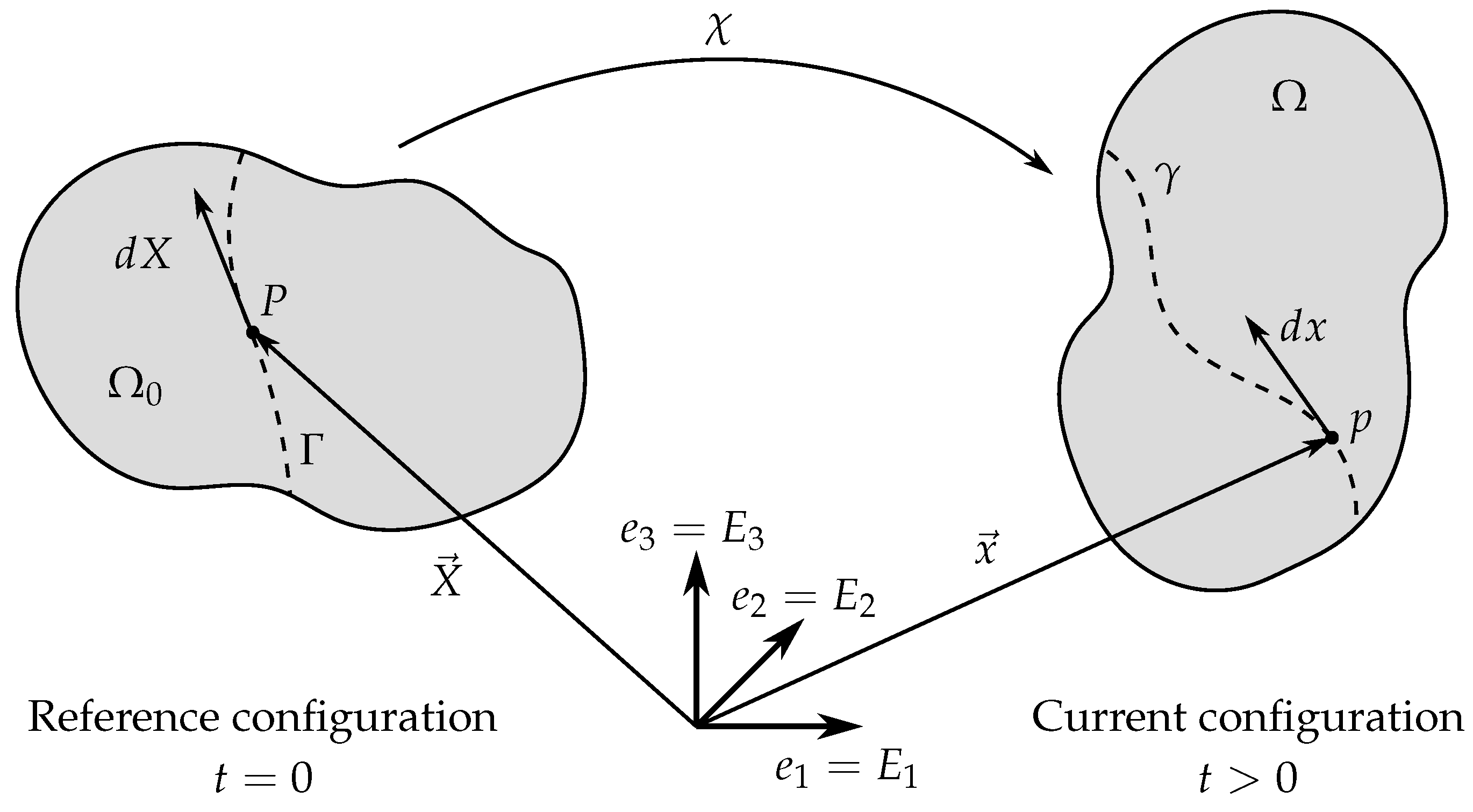
2.2. Kinematics
2.3. Mechanical Stress Definition
2.4. Magnetic Field Equations
2.5. Total Stress Tensor
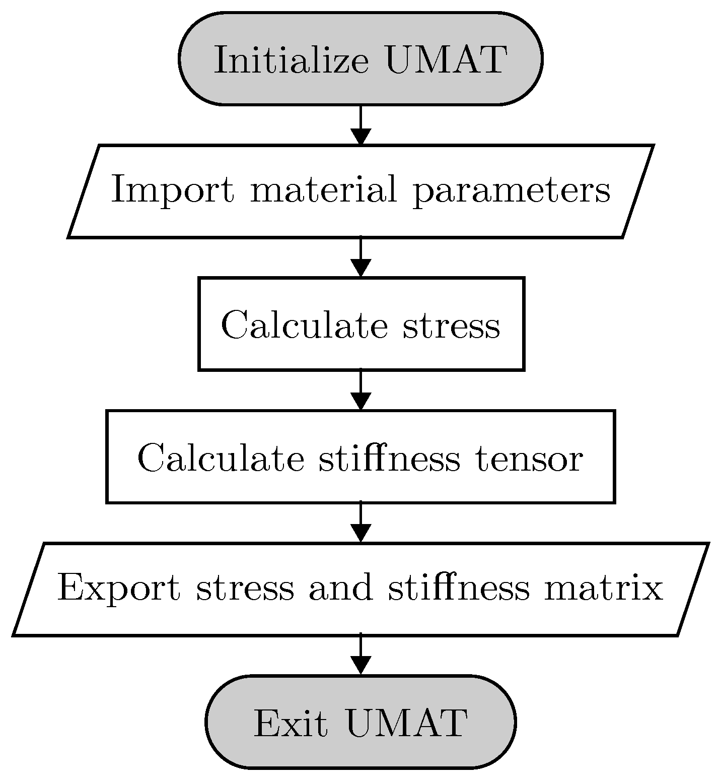
3. Implementation
3.1. Utilized Software Package
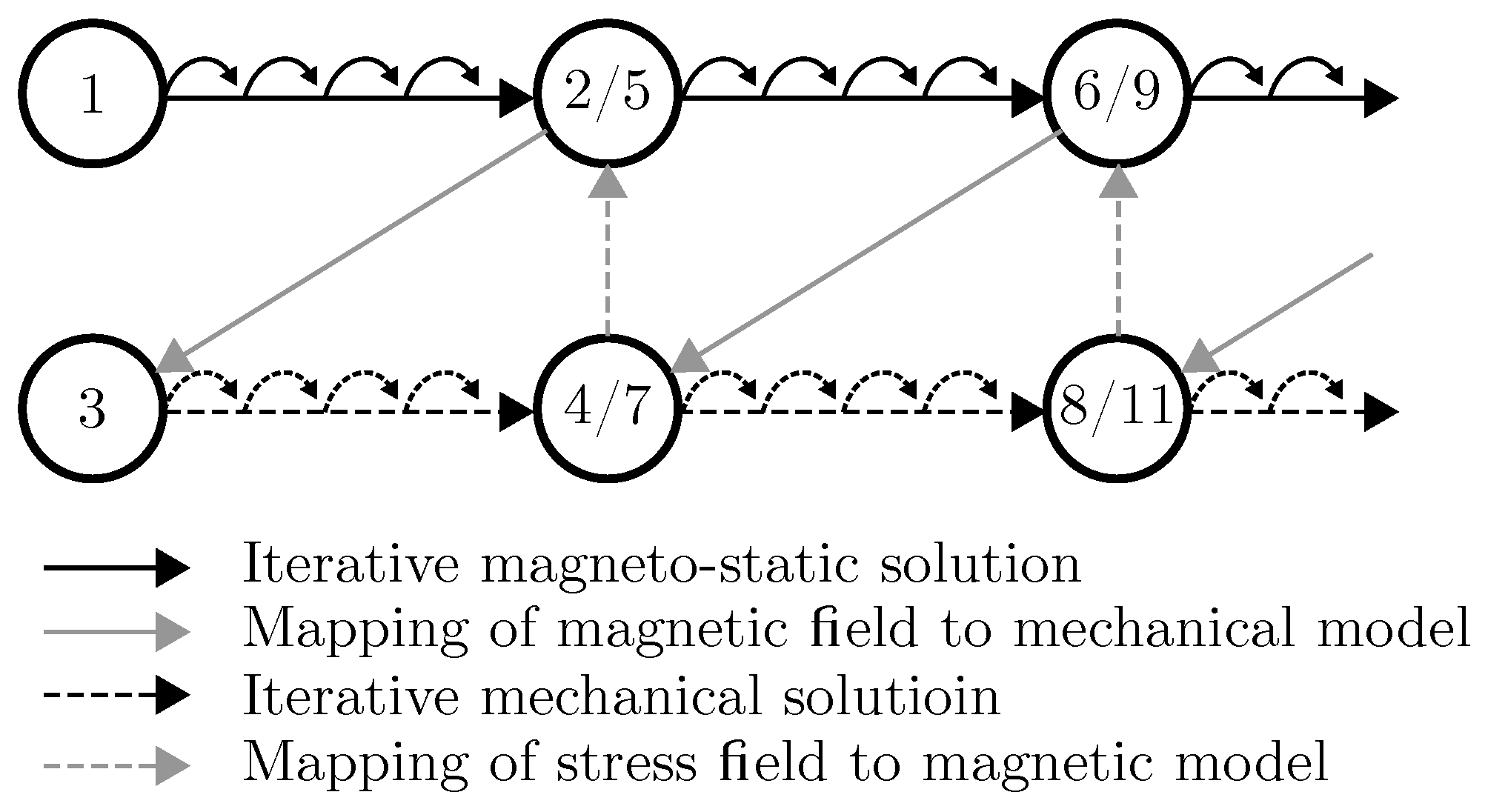
3.2. Iterative Coupling Method
- element orientation (e.g., corresponding to a pre-structuring direction),
- mapped magnetic field orientation,
- mapped magnetic field strength, and
- defined magneto-mechanical material behavior.
 .
.4. Discussion
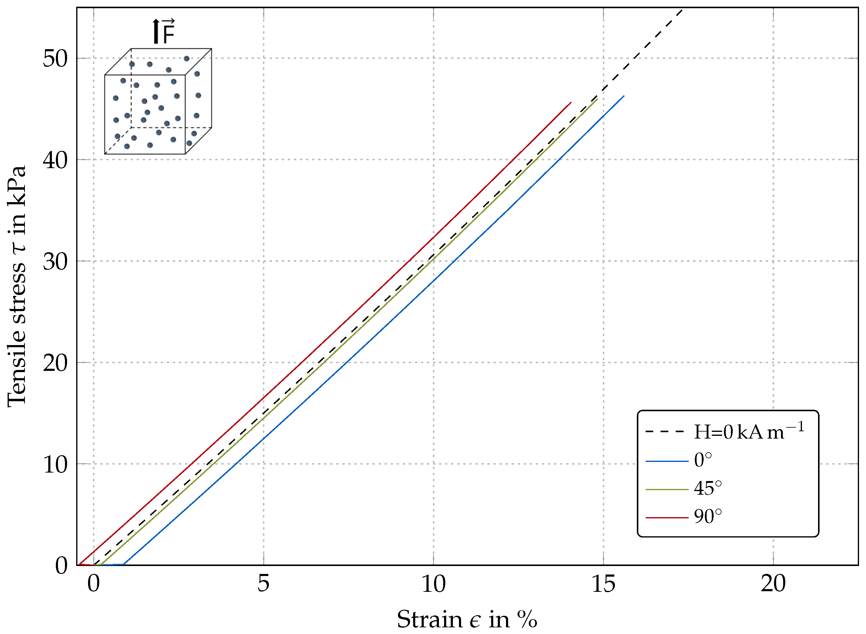
4.1. Simulation
4.1.1. Isotropic Model
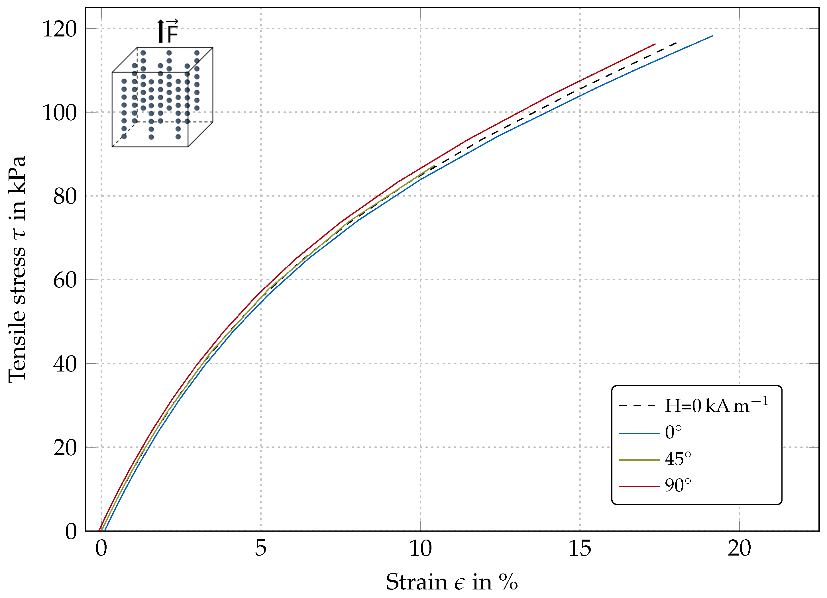
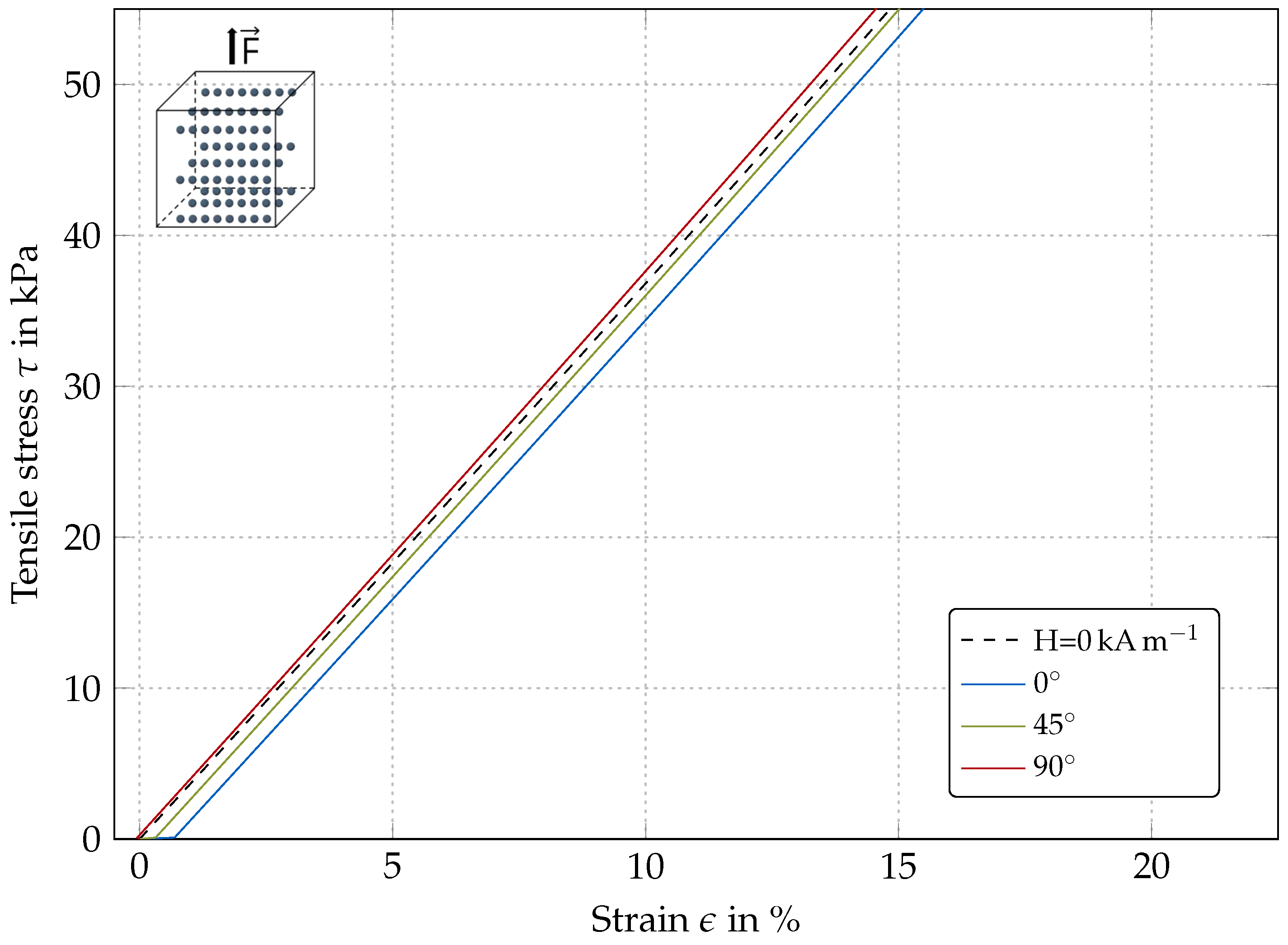
4.1.2. Transversely-Isotropic Models
4.2. Summary
5. Conclusions
Supplementary Materials
Author Contributions
Funding
Acknowledgments
Conflicts of Interest
Abbreviations
| MR | magnetorheological |
| MA | magneto-active |
| FE | finite element |
| UMAT | ABAQUS user material subroutine |
References
- Borin, D.; Stepanov, G.; Dohmen, E. On anisotropic mechanical properties of heterogeneous magnetic polymeric composites. Philos. Trans. R. Soc. A Math. Phys. Eng. Sci. 2019, 377, 20180212. [Google Scholar] [CrossRef] [PubMed] [Green Version]
- Bodelot, L.; Voropaieff, J.P.; Pössinger, T. Experimental investigation of the coupled magneto-mechanical response in magnetorheological elastomers. Exp. Mech. 2018, 58, 207–221. [Google Scholar] [CrossRef] [Green Version]
- Dohmen, E.; Borin, D.; Zubarev, A. Magnetic field angle dependent hysteresis of a magnetorheological suspension. J. Magn. Magn. Mater. 2017, 443, 275–280. [Google Scholar] [CrossRef]
- Wereley, N.M. (Ed.) Magnetorheology; RSC Smart Materials; The Royal Society of Chemistry: London, UK, 2014. [Google Scholar] [CrossRef]
- Dohmen, E.; Boisly, M.; Borin, D.; Kästner, M.; Ulbricht, V.; Gude, M.; Hufenbach, W.; Heinrich, G.; Odenbach, S. Advancing Towards Polyurethane-Based Magnetorheological Composites. Adv. Eng. Mater. 2014, 16, 1270–1275. [Google Scholar] [CrossRef]
- Kuzhir, P.; Bossis, G.; Bashtovoi, V.; Volkova, O. Effect of the orientation of the magnetic field on the flow of magnetorheological fluid. Part II. Cylindrical channel. J. Rheol. 2003, 47, 1385–1398. [Google Scholar] [CrossRef]
- Kuzhir, P.; Bossis, G.; Bashtovoi, V. Effect of the orientation of the magnetic field on the flow of a magnetorheological fluid. Part I. Plane channel. J. Rheol. 2003, 47, 1373–1384. [Google Scholar] [CrossRef]
- Li, Y.; Li, J.; Li, W.; Du, H. A state-of-the-art review on magnetorheological elastomer devices. Smart Mater. Struct. 2014, 23, 123001. [Google Scholar] [CrossRef]
- Odenbach, S. (Ed.) Magnetoviscous Effects in Ferrofluids; Springer: Berlin/Heidelberg, Germany, 2002; Volume 71. [Google Scholar]
- Linke, J.M.; Odenbach, S. Anisotropy of the magnetoviscous effect in a ferrofluid with weakly interacting magnetite nanoparticles. J. Phys. Condens. Matter 2015, 27, 176001. [Google Scholar] [CrossRef]
- Ambacher, O.; Odenbach, S.; Stierstadt, K. Rotational viscosity in ferrofluids. Z. Phys. B Condens. Matter 1992, 86, 29–32. [Google Scholar] [CrossRef]
- Grants, A.; Irbītis, A.; Kroņkalns, G.; Maiorov, M. Rheological properties of magnetite magnetic fluid. J. Magn. Magn. Mater. 1990, 85, 129–132. [Google Scholar] [CrossRef]
- Schliomis, M. Effective Viscosity of Magnetic Suspensions. Sov. Phys. JetP 1972, 34, 1291–1294. [Google Scholar]
- McTague, J.P. Magnetoviscosity of Magnetic Colloids. J. Chem. Physics 1969, 51, 133–136. [Google Scholar] [CrossRef]
- Gundermann, T.; Odenbach, S. Investigation of the motion of particles in magnetorheological elastomers by X-μCT. Smart Mater. Struct. 2014, 23, 105013. [Google Scholar] [CrossRef]
- Metsch, P.; Schmidt, H.; Sindersberger, D.; Kalina, K.; Brummund, J.; Auernhammer, G.; Monkman, G.; Kästner, M. Field-induced interactions in magneto-active elastomers—A comparison of experiments and simulations. Smart Mater. Struct. 2020. [Google Scholar] [CrossRef]
- Kalina, K.; Metsch, P.; Brummund, J.; Kästner, M. A Macroscopic Model for Magnetorheological Elastomers based on Microscopic Simulations. Int. J. Solids Struct. 2020, 193–194, 200–212. [Google Scholar] [CrossRef]
- Puente-Córdova, J.G.; Reyes-Melo, M.E.; Palacios-Pineda, L.M.; Martínez-Perales, I.A.; Martínez-Romero, O.; Elías-Zúñiga, A. Fabrication and Characterization of Isotropic and Anisotropic Magnetorheological Elastomers, Based on Silicone Rubber and Carbonyl Iron Microparticles. Polymers 2018, 10, 1343. [Google Scholar] [CrossRef] [Green Version]
- Metsch, P.; Kalina, K.A.; Brummund, J.; Kästner, M. A quantitative comparison of two- and three-dimensional modeling approaches for magnetorheological elastomers. PAMM 2018, 18, e201800179. [Google Scholar] [CrossRef]
- Bica, I. The influence of the magnetic field on the elastic properties of anisotropic magnetorheological elastomers. J. Ind. Eng. Chem. 2012, 18, 1666–1669. [Google Scholar] [CrossRef]
- Zhang, W.; Gong, X.L.; Chen, L. A Gaussian distribution model of anisotropic magnetorheological elastomers. J. Magn. Magn. Mater. 2010, 322, 3797–3801. [Google Scholar] [CrossRef]
- Kalina, K.A.; Metsch, P.; Kästner, M. Microscale modeling and simulation of magnetorheological elastomers at finite strains: A study on the influence of mechanical preloads. Int. J. Solids Struct. 2016, 102–103, 286–296. [Google Scholar] [CrossRef]
- Ivaneyko, D.; Toshchevikov, V.; Saphiannikova, M.; Heinrich, G. Effects of particle distribution on mechanical properties of magneto-sensitive elastomers in a homogeneous magnetic field. Macromol. Symp. 2012, 338, 96–107. [Google Scholar] [CrossRef]
- Jolly, M.R.; Carlson, J.D.; Muñoz, B.C. A model of the behavior of magnetorheological materials. SMart Mater. Struct. 1996, 5, 607. [Google Scholar] [CrossRef]
- Han, Y.; Hong, W.; Faidley, L.E. Field-stiffening effect of magneto-rheological elastomers. Int. J. Solids Struct. 2013, 50, 2281–2288. [Google Scholar] [CrossRef] [Green Version]
- Biller, A.M.; Stolbov, O.V.; Raikher, Y.L. Modeling of particle interactions in magnetorheological elastomers. JOurnal Appl. Phys. 2014, 116, 114904. [Google Scholar] [CrossRef]
- Bustamante, R. Mathematical Modelling of Non-Linear Magneto-and Electro-Active Rubber-Like Materials. Ph.D. Thesis, University of Glasgow, Glasgow, UK, 2007. [Google Scholar]
- Bustamante, R. Mathematical modelling of boundary conditions for magneto-sensitive elastomers: Variational formulations. J. Eng. Math. 2009, 64, 285–301. [Google Scholar] [CrossRef]
- Bustamante, R. Transversely isotropic nonlinear magneto-active elastomers. Acta Mech. 2010, 210, 183–214. [Google Scholar] [CrossRef]
- Bustamante, R.; Dorfmann, A.; Ogden, R.W. Numerical solution of finite geometry boundary-value problems in nonlinear magnetoelasticity. Int. J. Solids Struct. 2011, 48, 874–883. [Google Scholar] [CrossRef] [Green Version]
- Dorfmann, A.; Ogden, R.W. Nonlinear magnetoelastic deformations of elastomers. Acta Mech. 2004, 167, 13–28. [Google Scholar] [CrossRef]
- Brigadnov, I.A.; Dorfmann, A. Mathematical modeling of magneto-sensitive elastomers. Int. J. Solids Struct. 2003, 40, 4659–4674. [Google Scholar] [CrossRef]
- Varga, Z.; Filipcsei, G.; Zrínyi, M. Magnetic field sensitive functional elastomers with tuneable elastic modulus. Polymer 2006, 47, 227–233. [Google Scholar] [CrossRef]
- Filipcsei, G.; Csetneki, I.; Szilágyi, A.; Zrínyi, M. Magnetic Field-Responsive Smart Polymer Composites. In Oligomers–Polymer Composites–Molecular Imprinting; Springer: Berlin/Heidelberg, Germany, 2007; Chapter 3; pp. 137–189. [Google Scholar] [CrossRef]
- Abramchuk, S.; Kramarenko, E.; Stepanov, G.; Nikitin, L.V.; Filipcsei, G.; Khokhlov, A.R.; Zríínyi, M. Novel highly elastic magnetic materials for dampers and seals: Part I. Preparation and characterization of the elastic matrials. Polym. Adv. Technol. 2007, 18, 883–890. [Google Scholar] [CrossRef]
- Abramchuk, S.; Kramarenko, E.; Grishin, D.; Stepanov, G.; Nikitin, L.V.; Filipcsei, G.; Khokhlov, A.R.; Zríínyi, M. Novel highly elastic magnetic materials for dampers and seals: Part II. Material behavior in a magnetic field. Polym. Adv. Technol. 2007, 18, 513–518. [Google Scholar] [CrossRef]
- Hiptmair, F.; Major, Z.; Haßlacher, R.; Hild, S. Design and application of permanent magnet flux sources for mechanical testing of magnetoactive elastomers at variable field directions. Rev. Sci. Instruments 2015, 86, 085107. [Google Scholar] [CrossRef]
- Karrer, E.; Davies, J.M.; Dieterich, E.O. A simplified Goodrich plastometer. Ind. Eng. Chem. Anal. Ed. 1930, 2, 96–99. [Google Scholar] [CrossRef]
- Tang, X.; Conrad, H. Quasistatic measurements on a magnetorheological fluid. J. Rheol. 1996, 40, 1167–1178. [Google Scholar] [CrossRef]
- Dohmen, E.; Modler, N.; Gude, M. Anisotropic characterization of magnetorheological materials. J. Magn. Magn. Mater. 2017, 431, 107–109. [Google Scholar] [CrossRef]
- Holzapfel, G.A. Nonlinear Solid Mechanics: A Continuum Approach for Engineering; Wiley: Chichester, West Sussex, UK, 2010. [Google Scholar]
- Bustamante, R.; Dorfmann, A.; Ogden, R.W. On variational formulations in nonlinear magnetoelastostatics. Math. Mech. Solids 2008, 13, 725–745. [Google Scholar] [CrossRef]
- Ogden, R.W. Nearly isochoric elastic deformations: Application to rubberlike solids. J. Mech. Phys. Solids 1978, 26, 37–57. [Google Scholar] [CrossRef]
- Tanaka, M.; Fujikawa, M.; Balzani, D.; Schröder, J. Robust numerical calculation of tangent moduli at finite strains based on complex-step derivative approximation and its application to localization analysis. Comput. Methods Appl. Mech. Eng. 2014, 269, 454–470. [Google Scholar] [CrossRef]
- BELLAN, C.; BOSSIS, G. Field Dependence of Viscoelastic Properties of Mr Elastomers. Int. J. Mod. Phys. B 2002, 16, 2447–2453. [Google Scholar] [CrossRef]
- Stolbov, O.V.; Raikher, Y.L. Magnetostriction effect in soft magnetic elastomers. Arch. Appl. Mech. 2019, 89, 63–76. [Google Scholar] [CrossRef]
- Zubarev, A.; Chirikov, D.; Stepanov, G.; Borin, D. Hysteresis of ferrogels magnetostriction. J. Magn. Magn. Mater. 2017, 431, 120–122. [Google Scholar] [CrossRef]
- Ginder, J.M.; Clark, S.M.; Schlotter, W.F.; Nichols, M.E. Magnetostrictive Phenomena in Magnetorheological Elastomers. Int. J. Mod. Phys. B 2002, 16, 2412–2418. [Google Scholar] [CrossRef]

| Parameter | Value | Unit | Source |
|---|---|---|---|
| k | 1 | Table 1 in [29] | |
| Table 1 in [29] | |||
| /(/) | Table 1 in [29] | ||
| Table 2a in [29] | |||
| Table 2a in [29] | |||
| /(/) | Table 2a in [29] | ||
| /(/) | Table 2a in [29] | ||
| /(/) | Table 2a in [29] | ||
| /(/) | Table 2a in [29] | ||
| m | [29] (p. 197) |
| isotropic (no pre-structuring) | |
| pre-structuring direction parallel to field direction | |
| pre-structuring direction perpendicular to field direction |
Publisher’s Note: MDPI stays neutral with regard to jurisdictional claims in published maps and institutional affiliations. |
© 2020 by the authors. Licensee MDPI, Basel, Switzerland. This article is an open access article distributed under the terms and conditions of the Creative Commons Attribution (CC BY) license (http://creativecommons.org/licenses/by/4.0/).
Share and Cite
Dohmen, E.; Kraus, B. Coupled Anisotropic Magneto-Mechanical Material Model for Structured Magnetoactive Materials. Polymers 2020, 12, 2710. https://doi.org/10.3390/polym12112710
Dohmen E, Kraus B. Coupled Anisotropic Magneto-Mechanical Material Model for Structured Magnetoactive Materials. Polymers. 2020; 12(11):2710. https://doi.org/10.3390/polym12112710
Chicago/Turabian StyleDohmen, Eike, and Benjamin Kraus. 2020. "Coupled Anisotropic Magneto-Mechanical Material Model for Structured Magnetoactive Materials" Polymers 12, no. 11: 2710. https://doi.org/10.3390/polym12112710