1. Introduction
Over the years, research involving the blending of different pseudo-spherical particle sizes to maximize the packing fraction has been addressed to optimize several physical properties including viscosity [
1,
2,
3,
4,
5,
6,
7,
8,
9,
10,
11,
12,
13,
14,
15,
16,
17,
18,
19,
20,
21,
22,
23,
24,
25], modulus [
26,
27,
28,
29,
30,
31,
32,
33,
34], and impact [
35,
36,
37,
38,
39,
40,
41,
42]. The importance of the packing fraction for a property such as viscosity can easily be evaluated by addressing one of the more general models to characterize viscosity, such as the following generalized viscosity model [
7,
8,
9,
10]:
where
η = suspension viscosity;
ηo = viscosity of suspending medium;
[η] = intrinsic viscosity;
σ = interaction coefficient;
λPC = particle–particle component of the interaction coefficient;
σs = solvent–particle component of the interaction coefficient;
φ = particle volume fraction concentration;
φn = particle packing fraction;
= number average particle size or the first moment average particle size.
While optimizing the packing fraction is important for large-scale pseudo-spherical aggregates such as asphalt applications, there are also many other applications for optimizing particle size distributions on a much smaller scale. Many small-scale particle size analyzers maintain a constant ratio between successive particle sizes analyzed, Z, such as for the LS 130 Coulter Counter where Z = 1.09532. For reference, the maximum range of particles that can be indicated using the LS 130 Coulter Counter is only from 0.1 microns to 899.7 microns. For such a particle size analyzer, it is normally found that each i
th particle group of diameter
Di in a particle distribution can then be evaluated (where, in general, Z > 1) as:
where
Several attempts have been made over the years to elucidate the best theoretical [
8,
9,
10,
41,
43,
44,
45,
46,
47,
48,
49] approach to characterize the blending of different pseudo-spherical particle sizes to maximize the packing fraction. Based on experimental considerations, Kaeuffer [
49] found that the optimum particle size distribution for a pigment in a paint would be achieved when the accumulated volume fraction for the distribution was directly proportional to the square root of the particle diameter. In other words, according to Kaeuffer, the accumulated volume fraction from the smallest particle size up to the largest particle size considered, D
β, was assumed to be dependent on the square root of the particle diameter as:
where:
Sudduth [
8,
9,
10] was able to extend the experimental observations found by Kaeuffer by showing theoretically that the volume fraction for the i
th particle size in an optimum particle size distribution can be calculated as:
where:
Vi = volume of the ith particles;
VT = total volume of all particles;
fi = volume fraction of particles of the ith type.
Sudduth [
44] also found that for volume fractions calculated using Equation (5) with a constant ratio between particle sizes, a straight line of the following form would necessarily result:
Note specifically that the straight line described by Equation (6) typically does not necessarily go through the origin.
In addition, as already indicated, several attempts have been made over the years to elucidate the best theoretical [
8,
9,
10,
41,
43,
44,
45,
46,
47,
48,
49] approach to characterize the blending of different pseudo-spherical particle sizes to maximize the packing fraction. The theoretical analyses then required extensive experimental blending data [
50,
51,
52] to maximize the packing fractions from several different particle size distributions to compare with the theoretical models.
Probably the most extensive empirical study for blending different particle sizes was generated by McGeary [
52] to maximize the packing fraction in fuel rods for use in nuclear generated power plants.
The experimental results from McGeary have then be utilized in this study to identify how Equations (5) and (6) can be generated theoretically. The theoretical background used to generate Equations (5) and (6) also resulted in the identification of a ratio of two specific particle size averages that has been particularly successful in indicating the packing effectiveness of any given particle size distribution.
At this point, it is useful to identify how to best develop an optimum distribution described by the straight line requirement, as indicated by Equation (6). This study will address the practical limits for the two dominant fundamental approaches to designing particle size distributions to address a specific physical property such as viscosity. Two fundamental approaches to obtain such a straight line would include:
- (1)
The first design approach would be generated utilizing the same initial particle size, Dmin, but by using different ultimate particle sizes, Dmax.
- (2)
The second design approach would be generated where each distribution starts with the same initial particle size, Dmin, and ends with the same ultimate particle size, Dmax.
The first design approach is particularly useful to identify the possible slopes available based on the smallest available particle size and the largest available particle size that can be used in the particle blend for a specific application. Once the slope has been identified, the second design approach can be utilized to identify the preferred ratio between particles, Z, and the number of different particle sizes, n, to be utilized in the final particle blend.
2. Particle Size Distribution Concepts from an Analysis of McGeary’s Particle Size Distributions
Probably the most extensive particle size blending study for spherical particles was generated by McGeary [
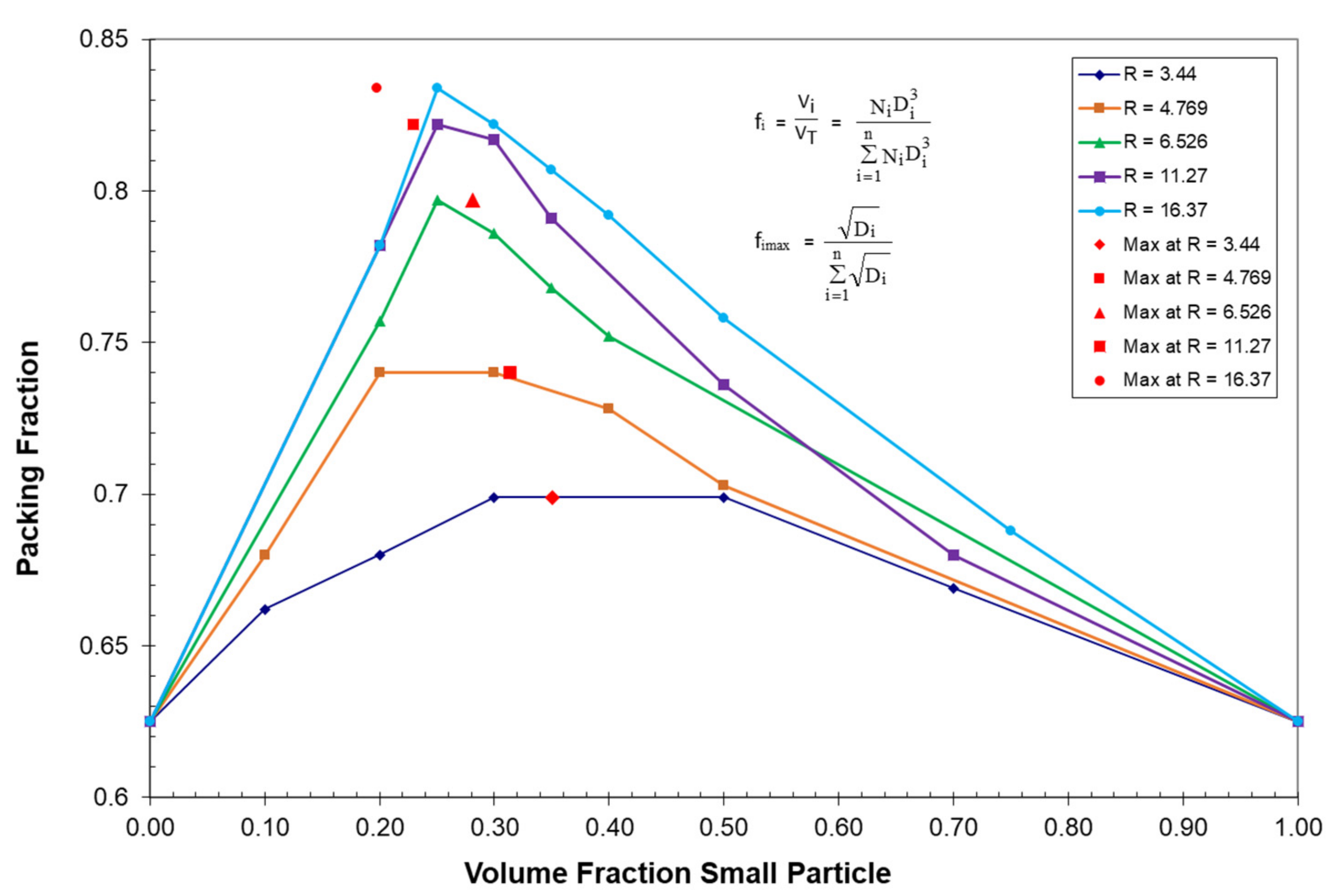
52] as a result of his effort to maximize the packing fraction for fuel rods utilized in nuclear generated power plants. The packing fraction for five binary sets of McGeary’s blending data for spherical particles have been plotted in
Figure 1 as a function of the volume fraction of the smallest particle. The volume fraction for each particle, f
i, in
Figure 1 can be described as:
Taking the ratio of two volume fractions yields:
Assuming that N
k = 1 for largest particle diameter, then the first moment,
, and the fifth moment,
, average particle sizes can be calculated as:
where:
Vi = volume of the ith particles;
Vk = volume of the kth particles;
VT = total volume of all particles;
fi = volume fraction of particles of the ith type;
fk = volume fraction of particles of the kth type;
= number average particle size or the first moment average particle size;
= fifth moment average particle size;
Ni = number of particles of the ith particle size;
Di = diameter of the ith particle size;
n = number of different particle sizes in mixture.
Using Equations (7)–(11), the ratio
/
particle size averages for McGeary’s five binary particle size distributions have been plotted in
Figure 2 as a function of the volume fraction of the smallest particle. The theoretical maximum value of
/
included in each of the binary plots
Figure 1 and
Figure 2 has previously been shown [
8,
10] to easily be calculated as:
Note that the maximum volume fraction, fimax, for component i can be calculated as the square root of diameter i divided by the sum of the square roots of all particle diameters in the distribution.
Of all possible ratios, it has been shown in a previous extensive study [
8] that only the
/
ratio of average particle sizes can accurately predict both the location and relative magnitude of the maximums for McGeary’s [
52] five binary particle size distributions as indicated in both
Figure 1 and
Figure 2. In a later study [
10], it was further established that Equation (12) also applies to the calculation of the volume fraction for any particle size at the maximum packing fraction independent of how many different particles have been included in the particle size distribution.
The maximum packing fraction found by McGeary [
52] for several particle size distributions from binary blends to distributions with up to four particles has been summarized in
Table 1. Note that, using Equation (12), the calculated volume fractions yielding the maximum packing fractions for McGeary’s distributions in
Table 1 were found [
8] to be in good agreement with the volume fractions that McGeary found experimentally.
Since monodisperse spherical particles have essentially the same packing fraction, φ
m, independent of their particle size, then smaller particles can then fit in between the larger particles. In general, Lee [
46] has indicated that monodisperse spherical particles have a maximum packing fraction of φ
m = 0.589 for loose random packing and φ
m = 0.639 for dense random packing. If the assumption is made that smaller spheres will fit into the voids left by the larger spheres, then the ultimate maximum packing fraction, φ
nult, for n different particle sizes yields the following equation, which has been previously published [
8] in detail, has been summarized in
Appendix A:
For reference, the ultimate packing fraction has been summarized in
Table 2 for up to 12 different particles for both loose random packing and for dense random packing. For reference, it needs to be noted that the maximum possible value for
cannot be greater than the magnitude of the largest particle diameter in the distribution and the minimum possible value for
cannot be smaller than the magnitude of the smallest particle diameter in the distribution. The ultimate packing fraction, φ
nult, described by Equation (13) is also shown in
Figure 3 along with the maximum packing fractions that were established experimentally by McGeary’s distributions as indicated in
Table 1. Note in
Figure 3 how amazingly close McGeary’s experimental results were to the ultimate theoretical packing fraction.
At this point, the maximum packing fraction for any particle size distribution then can be calculated using the following equation, which has been developed in a previous publication [
8]:
where:
φn = particle packing fraction;
φnult = ultimate Particle packing fraction;
φm = monodisperse particle packing;
α = particle size distribution constant = 0.268;
= number average particle size or the first moment average particle size;
= fifth moment average particle size.
This equation for the maximum packing fraction, φ
n, was required to be a function of the ratio
/
to successfully predict the maximums for McGeary’s additional blends for tertiary and quaternary blends as well as indicated in
Table 1. It has also been found that Equation (14) has also been successfully extended to include blends with an indefinite number of particles as well.
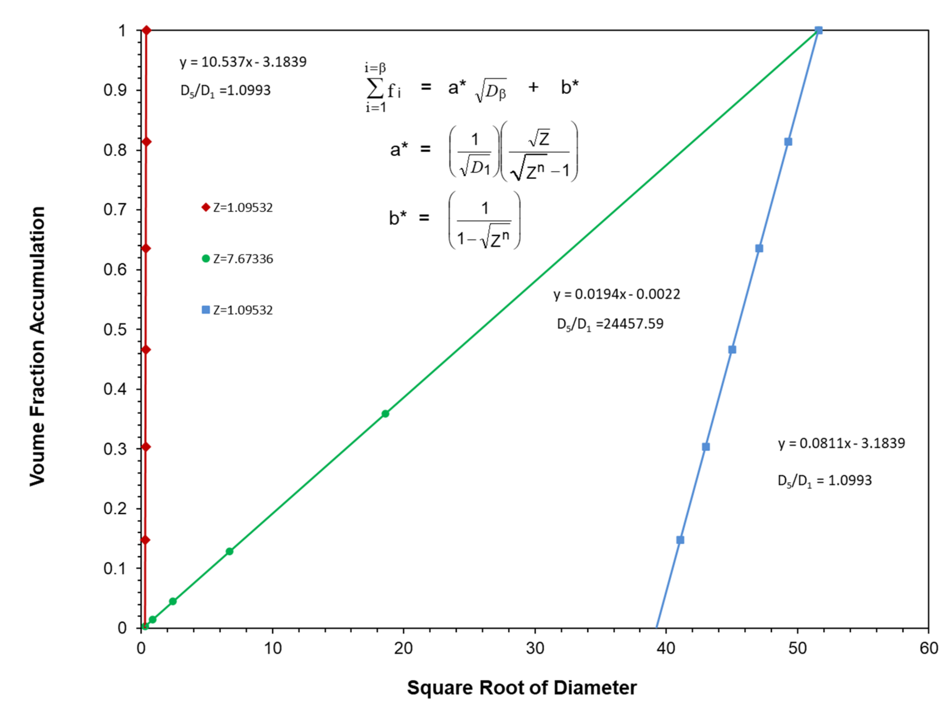
It has also been found that the accumulated volume fractions at the maximum packing fraction for three of McGeary’s particle size distributions can be plotted as effective straight lines as a function of the square root of the particle diameter as indicated in
Figure 4 and
Figure 5 as well as in
Table 3. The following equations were used to obtain the straight lines indicated in
Figure 4 and
Figure 5 as the results in
Table 3:
The correlation between the McGeary’s experimental results and the calculated results in
Figure 4 and
Figure 5 as well as in
Table 3 were quite remarkable. This again suggested that the calculated results appear to be approaching the correct theoretical explanation of McGeary’s experimental results.
Finally, it should be noted that the ratio between McGeary’s particles sizes as indicated in
Table 1 ranged from 5.55 to 11.27. Consequently, it was of interest to see if there was an optimum ratio that would be preferred between particle sizes. The resulting derivation of the optimum ratio between particles, which has been generated in a recent publication [
43], simply looked at the particle ratio between the maximum packing fraction between n and n+1 particles as described by Equation (13). An outline of this derivation which resulted in the following equation has been summarized in
Appendix B:
Equation (18), as derived in
Appendix B, indicates that the optimum ratio between particles, Z
Optimum, should be a direct function of the monodisperse packing fraction for spheres, φ
m. Again, note that Lee [
46] found that for loose random monodisperse packing of spheres (φ
m = 0.589), whereas for dense random monodisperse packing of spheres (φ
m = 0.639). Consequently, the optimum Z results summarized in
Table 4 have been calculated for monodisperse packing fractions that range from loose random packing to dense random packing. As indicated in
Table 4, values of the optimized ratio between particles would then appear to range between 5.92 and 7.67, which is approximately the same range as that found by McGeary experimentally, as indicated in
Table 1. In general, the agreement between theory and McGeary’s experimental results appears to be quite good.
Consequently, it is of interest to include the following quote from the final statement that McGeary [
52] made in his conclusion to his study:
“To produce efficient packing, there should be at least a sevenfold difference between sphere diameters of the various individual components. This size difference was shown to be associated with the ‘triangular pore size’ in the established packing through which the next component had to migrate to reach a permanent site.”
This result again indicates that the results that McGeary found experimentally agree very nicely with the theoretical analysis of his results as addressed in this study.
3. Influence of the Maximum Packing Fraction on the Generalized Viscosity Model
The generalized viscosity model introduced earlier in Equations (1) and (2) as well as Equations (7)–(14) were developed by Sudduth [
7,
8,
9,
10] to describe the viscosity of suspensions and composites with spherical particles as a function of the pigment volume concentration, φ. Three primary variables—the intrinsic viscosity, [η]; the maximum packing fraction, φ
n; and an interaction coefficient, σ—were included in the original development of the generalized viscosity equation. As indicated in
Table 5, the modification of the interaction coefficient, σ, can characterize the solubility of the suspended phase [
53,
54,
55].
The modification of the interaction coefficient, σ, can also be adjusted to yield several different well known suspension equations. For example, when σ = 0, the Arrhenius [
23] equation results; when σ = 1, the Krieger–Dougherty [
24] equation results; and when σ = 2, the Mooney [
25] equation results.
As indicated in
Figure 6, an adjustment of the interaction coefficient to yield a change in the suspension solubility would also typically result in a change in the shape of the viscosity curve, as indicated in
Figure 6. Note that curves in
Figure 6 were all calculated using the Einstein limit [
21,
22] for the intrinsic viscosity of [η] = 2.5 with a maximum packing fraction of φ
n = 0.59.
Similarly, the results in
Figure 7 were calculated with a range of values for the maximum packing fraction, again using the Einstein limit for the intrinsic viscosity of [η] = 2.5 but with a constant interaction coefficient of σ = 1.01. The results in
Figure 7 then suggest that the viscosity of suspensions can be significantly reduced at higher concentrations by increasing the maximum packing fraction of the particle size distribution. In other words, increasing the maximum packing fraction to reduce viscosity, as indicated in
Figure 7, has similar characteristics to decreasing the interaction coefficient to modify the solubility of the suspended particles, as indicated in
Figure 6.
4. Extension of the Influence of the Slope and Intercept of Straight Line for the Optimum Particle Size Distribution with Improved Blending Considerations
Many particle size analyzers maintain a constant ratio, Z, between successive particle sizes analyzed such as that for the LS 130 Coulter Counter where Z = 1.09532. For such a particle size analyzer, it is normally found that each i
th particle group of diameter D
i in a particle size distribution can then be evaluated (where, in general, Z >1) as:
Rearranging then also gives:
and
where:
Note that the maximum range of particles that can be indicated using the LS 130 Coulter Counter is from 0.1 microns to 899.7 microns. It can easily be shown using Equation (19) that the maximum number of different particle size groups that can then be analyzed with this machine is n = 101.
As described earlier, Equation (6) can be used to describe an optimum particle size distribution with a straight line as:
The values for a* and b* in Equation (23) can then be directly calculated based on the following two boundary conditions:
For n = 1, D
β = D
1 = D
Min and
It has also been shown in
Appendix C that the sum
reduces to:
Combining Equation (C4) as well as Equations (20), (24) and (25) with Equation (23) yields:
Note that Equation (26) indicates that the slope for the straight line will always be positive. Conversely, Equation (27) indicates that the value of the straight line intercept, b*, can never be positive. However, recall that for McGeary’s data using Equation (17) the straight line intercept, b**, can be positive if:
At the maximum packing fraction for a particle size distribution, the ratios of two maximum volume fractions can be obtained by combining Equations (8) and (12) to give:
If N
kmax = 1 for the largest particle at the maximum packing fraction, then the relative number of smaller particles for the i
th particle size indicated by N
imax can be easily calculated. In a previous article [
41], it was also shown that at the optimum composition for an optimum distribution that the general particle size average,
, can calculated as
Further simplification similar to that described in
Appendix C yields:
Consequently, at the optimum composition for an optimum particle size distribution, the averages of and can be easily calculated using Equation (32) as well as Equations (10) and (11) to yield the ratio /. Note that the ratio / calculated using Equation (32) is dimensionless and is only a function of Z and n.
The limiting
particle size average that would be of interest depends primarily on which physical property is desired to be addressed. For example, it has already been indicated that to address the viscosity [
7,
8,
9,
10] and/or modulus [
26], both the first moment or number average particle size,
, and the fifth moment average particle size,
, would be need to be evaluated. However, to address an impact performance [
41,
42], the surface average particle size,
, would be of interest and could readily be calculated.
5. Influence of the of the Ratio between Particle Sizes, Z, on the Slope, Maximum Packing Fraction, φn, and the Average Particle Size Ratio /
In general, the optimum packing fraction, φn, as described by Equation (14) would be expected to increase with an increase in the magnitude of the ratio of two specific average particle sizes, namely the ratio of /. This study has addressed several new approaches to evaluate the / ratio. In general, the larger the ratio of / evaluated from particle size distribution measurements, typically, the better the packing of that particle size distribution. Most instruments that measure particle size distribution characterize the distribution with measured values of the volume fraction, fi, and/or the relative numbers, Ni, for each diameter of the ith particle size, Di.
The five examples of optimal straight line particle size distributions illustrated in
Figure 8 have been generated using Equations (23), (26) and (27) with each distribution starting at the same initial particle size at D
1 = D
Min = 0.1 microns. The straight line for each distribution in
Figure 8 then had just six particles that were generated using a different ratio between particles, Z, and each ended at a different particle size, D
Max, generated as the sixth particle.
The calculated results for the distributions in
Figure 8 are summarized in
Table 6 and
Figure 9 along with an extra distribution that was not included in
Figure 8.
There are several observations of interest in
Table 6, including:
Note that as the value of Z was increased, the slope continued to decrease while the ratio of
/
continued to increase, as indicated in
Figure 9. This result was consistent with the earlier observations with McGeary’s data in
Table 1 as well as in
Figure 4 and
Figure 5.
However, note that while the value of the maximum packing fraction, φ
n, in
Table 6 calculated using equation 14 was quite low at low values of the ratio
/
it did increase with an increase in the ratio
/
and ultimately approached an upper limit.
Finally, the intercept, b*, also had a tendency to increase with an increase in the value of Z. At this point, the value of the intercept does not appear to be as significant as the change in the value of the slope in trying to optimize the packing fraction since it generally seems to have a value near b* = 0.
To better interpret the results summarized in
Table 6 as well as the results in
Figure 8 and
Figure 9, it is important to review the limits of the ultimate maximum packing fraction, φ
nult, and the maximum packing fraction, φ
n, as influenced by the number of different particles, n, in the particle size distribution and the average particle size ratio,
/
. An initial discussion of the number of different particles, n, on the ultimate maximum packing fraction, φ
nult, were previously indicated earlier in
Table 2 and
Figure 3 in association with the experimental data of McGeary. With loose random packing and only 2 particles in the blend then the results in
Table 2 and
Figure 3 indicated that an upper limit maximum packing fraction of only φ
n = 0.8311 can be achieved even with the maximum possible ratio of
/
.
Figure 10 addresses the relationship between the maximum packing fraction, φ
n, and the average particle size ratio,
/
, as a function of the number of particles, n, in the blend. Note in
Figure 10 that only lower values of the maximum packing fraction are possible for all particle combinations for up to six particles if the value of
/
is less than 10. Reference back to
Figure 7 also indicates that if the maximum packing fraction cannot achieve above φ
n = 0.6 that a possible improvement in viscosity at higher concentrations is minimized.
Two of the three optimum straight line distributions with six particles included in
Figure 11 were previously included in
Figure 8. However, the third six-particle optimum distribution in
Figure 11 had a very different starting particle size with the remaining five particles being generated with a ratio between particles of Z = 1.0953. The results of the calculations for the three particle size distributions in
Figure 11 have been included in
Table 7. The two particle size distributions in
Figure 11 with the same ratio between particle sizes of Z = 1.0953 and the same number of particles, 6, both ended up with the same value of the ratio of
/
, even though they had very different starting particle sizes. However, the two distributions in
Figure 11 with the same ratio between particles of Z = 1.0953 and the same ratio of
/
had significantly different slopes. This is a clear case wherein the distribution with a higher value of
/
did not yield a lower slope. These two cases with different slopes and different starting particle sizes indicated that the ratio
/
would appear to be considerably more important than the value of Z in controlling the maximum packing fraction.
Nevertheless, the results from
Figure 8,
Figure 9,
Figure 10 and
Figure 11 and
Table 6 and
Table 7 did indicate that it appears to be very desirable to maximize the difference between the minimum size particle,
D1 =
DMin, and the maximum size particle,
DMax, when trying to maximize the ratio of
/
and minimize the slope. It would also appear to be desirable to have at least six or more different particles in an optimum blend to be able to have the possibility to maximize the upper limit maximum packing fraction. For such an optimal particle size distribution, an increase in the value of
/
normally yields an increase in the maximum packing fraction, φ
n, as well as a lower slope. However, the range between the minimum particle size and the maximum particle size would be expected to depend significantly on the application of interest as well as other properties that may be desired.
6. Effect of a Constant Slope on the Influence of the of the Ratio between Particle Sizes, Z, Maximum Packing Fraction, φn, and the Average Particle Size Ratio /
Once the desired maximum and minimum particle sizes have been generated, the slope of the desired particle size distribution would have been established, as shown by the example in
Figure 12. At this point, it is desirable to evaluate the number of different particles to be in the distribution as well as the ratio between particle sizes. The relation between the number of particles and the value of Z to be used is clearly indicated using either Equation (21) or (22) once the maximum and minimum particle sizes have been identified so that all of these combinations have the same slope.
The results indicated in
Table 8 mathematically describe the relationship between the number of particles and their corresponding Z values for these straight lines with essentially the same slope as the straight line in
Figure 12. The results in
Table 8 have identified particle size distributions with the same slope but different combinations between the number of particles, n, and the ratio between particle sizes, Z.
All of the slopes and intercepts in
Table 8 were calculated using Equations (21) and (22) after first relating the number of particles, n, and Z using Equations (26) and (27). However, it is interesting that while this same process was used for all the calculations in
Table 8, the slopes seem to be decreasing ever so slightly in magnitude as the value of Z is increased. This result has no explanation at this point.
Note that the values of Z in
Table 8 have been plotted as a function of the number or particles, n, in
Figure 13.
In order to understand the results in
Figure 13, it is first important to point out that there is an optimum ratio between particles, as addressed in
Appendix B.
Appendix B addresses the derivation [
43] of the optimum ratio between the ultimate packing fractions described in
Appendix A. The final result in
Appendix B is Equation (B10), which is:
The calculated results using Equation (B10) as previously discussed and summarized in
Table 4 yielded a range of this optimum ratio between particles of 5.9199 ≤ Z
Optimum ≤ 7.6734. It is apparent in
Figure 13 that the location of these optimum values for Z is where the curve increases sharply.
The maximum packing fractions in
Table 8 have also been plotted in
Figure 14 as a function of the number of particles in the blends. As indicated in
Figure 14, there is a sharp drop in the maximum packing fraction when the number of particles in the distributions drops below 10. It is also important to note in
Table 8 that the ratio of
/
continues to increase unabated as the number of particles in the distribution decreases from 86 to 2.
Note that optimum Z values of 5.9199 and 7.6734 have been included in both
Table 6 and
Table 8. In
Table 6, these values for Z were both applied to the same number of particles in the blend. However, in
Table 8, these same values of Z were applied to a constant slope analysis of the blend. The availability of both of these approaches as outlined in
Table 6 and
Table 8 can be potentially useful when optimizing a particle size distribution for a specific application.
Another important observation in
Table 8 is the change in the volume fraction of small particles as the number of different particles in the blend is decreased. For reference, the volume fraction of particles in
Table 8 has also been recalculated as the number of small particles relative to the total number of particles in the blend. Note that the volume fraction of the smallest particles has only increased from a volume fraction of 0.00095 to 0.0204 in going from 86 particles to 2 particles. However, as indicated in both
Table 8 and
Figure 15, the number fraction of the smallest particles increased from 0.203 to approximately 1.000 as the number of particles decreased from 86 particles to 2 particles.
The increase in the number of small particles can also play a significant detrimental role in modifying a property such as viscosity.
In general, the volume of a sphere vs. can be obtained as:
where r = sphere radius.
In addition, the surface area of a sphere, A
s, can be obtained as:
The ratio of surface to volume is then:
As the diameter of a sphere becomes smaller, the surface-to-volume ratio of the small particles can contribute dramatically as the number of small particles increase. This can be important since the interaction coefficient, σ, in the generalized viscosity model [
7,
8,
9,
10] can be described by Equation (2) as:
where
= number average diameter of particles in the blend.
Consequently, as the number of small particles in the blend increases, the interaction coefficient can increase significantly as a result of an increase in the surface to volume of the particles, which, in turn, can increase the viscosity as indicated in
Figure 6. This is then another significant reason to have a large number of different-sized particles in the blend to minimize the possibility of having an increase in viscosity as a result of having too many small particles.
In general, as indicated in
Figure 10, a minimum of six particles should be included in the final particle blend to be able to maximize the packing fraction. Utilizing the results in
Figure 10 along with the other equations in this study, the possibility of using only six particles to generate an effective optimum particle size distribution has been addressed in
Table 9. Note in
Table 9 that when only six particles are in the distribution and the ratio between particles is Z = 1.0953, a maximum ratio of
/
= 1.099 is obtained. As indicated in
Figure 10, a ratio
/
= 1.099 would obviously be quite inadequate.
Consequently, based on the results in
Figure 10, it would generally be undesirable to generate an optimum particle size distribution if the ratio of
/
< 25. Therefore, as indicated in
Table 10, a minimum requirement of
/
≥ 25 would be a strongly recommended for an optimum particle size distribution to achieve an effective maximum packing fraction. In general, blends with less than six particles would need to be adjusted extremely carefully to make sure that whatever property (such as viscosity) is addressed, the property will not be adversely affected.
8. Conclusions
This study has identified several practical limits to address the two dominant fundamental approaches to designing optimum particle size distributions with a maximum packing fraction. For a property such as viscosity, if the maximum packing fraction cannot reach above φn = 0.6, the possibility of lowering the viscosity at higher particulate concentrations is significantly reduced. At maximum packing fractions such that φn > 0.6, the generalized viscosity model has indicated that the viscosity at higher concentrations can be reduced since a higher packing fraction can act similarly to reducing the interaction coefficient. However, it has also been shown that if there is a large difference in the sizes of the particles, if there are fewer than six particles, and if the ratio of / is less than 10, then it has been shown that too many small particles can cause the viscosity to increase. An increase in the number of small particles associated with an increase in the surface-to-volume ratio of small particles can play a significant role in modifying or degrading a property such as viscosity.
Based on a detailed analysis of McGeary’s extensive study of several binary, tertiary, and quaternary particle size distributions, it has been found that the maximum packing fraction appears to be fundamentally related to the average particle size ratio /. Two important observations identified from a detailed analysis of McGeary’s extensive study included:
- (1)
Of all the possible ratios of average particle sizes only the ratio of the fifth moment to the first moment average particle sizes, /, was able to effectively characterize both the relative magnitude and the location of the maximum packing fraction for each of McGeary’s binary, tertiary, and quaternary particle size distributions.
- (2)
The location of the maximum value of the ratio, /, at the maximum packing fraction was obtained when the volume fraction for each particle size in the distribution was calculated from the square root of the particle diameter divided by the sum of the square roots of all the particle diameters in the distribution.
At the maximum packing fraction for an optimum constant ratio particle size distribution, a plot of accumulated particle volume fractions vs. square root of particle diameter will normally yield the following characteristics:
For an optimum particle size distribution with a constant ratio between particle sizes, Z, a plot of the accumulated volume fraction vs. the square root of the particle size will, out of necessity, form a straight line with the following characteristics.
If the value of Z >1, then the slope, a*, will be positive and the intercept, b*, will be negative.
The magnitude of the optimum maximum packing fraction is normally increased when the ratio of / has been increased and the slope of the straight line has been lowered.
For the same ratio between particles, Z, and the same number of particles, n, the ratio of / will normally remain the same independent of the value for the initial or minimum particle size, Dmin.
For the same ratio between particles, Z, if the particle distribution has the same initial particle size, Dmin, and the maximum particle size, Dmax, has been increased, the ratio of / must necessarily increase and the slope will normally decrease.
An increase in the ratio between particles, Z, normally results in an increase in the ratio of / with a decrease in the number of different particle sizes, n, and the relative volume fraction of the smallest particle size will normally necessarily increase.
In general, an optimum particle size distribution can be generated if the volume fractions for a particle size distribution are calculated from the square root for each particle diameter divided by the sum of the square roots of the particle diameters, even if there is not a constant ratio between particles. However, if there is not a constant ratio between particle sizes, then such an optimum particle size distribution may only generate an approximate straight line for the accumulated sum of the volume fractions vs. the square root of the particle size. For such an approximate straight line such as was obtained for McGeary’s experimental data that did not necessarily have a constant ratio between particles, it was found that the intercept b** can be positive when:
The two dominant fundamental approaches to designing optimum particle size distributions with a maximum packing fraction can be described as:
- (1)
The first design approach would be generated utilizing the same initial particle size, Dmin, but by using different ultimate particle sizes, Dmax.
- (2)
The second design approach would be generated where each distribution starts with the same initial particle size, Dmin, and ends with the same ultimate particle size, Dmax.
For small-scale particle-size distributions measured with an instrument such as a Coulter Counter, typically, the measured volume fractions are generated with a constant ratio between particle sizes. In this case, once the minimum and maximum particle sizes have been established, the ratio / can be maximized by blending several particle size distributions to an identified straight line to generate the desired final particle size distribution.
It was also found that there is a theoretical optimum ratio between particles, ZOptimum, which appears to range from 5.9199 ≤ ZOptimum ≤ 7.6734. This range of ratios was approximately the same range that McGeary found to be optimum in his study as well. This result indicated that these theoretical calculations agreed nicely with McGeary’s extensive experimental results.
The disadvantage of many particle counters is that their value of Z is often limited to a value not much greater than Z = 1 such as the Coulter Counter with Z = 1.0953. Such a blending approach often requires large numbers of particles to be in the blend to be effective. However, such blends can often be carried out very quickly with a computer program.
While particle counters can be effective when utilized properly, the value of Z can be improved significantly by using multiple sieves to generate optimum particle size distributions.


