
Numerical Study for the Performance of Viscoelastic Fluids on Displacing Oil Based on the Fractional-Order Maxwell Model
Abstract
:
1. Introduction
2. Physical and Mathematical Models
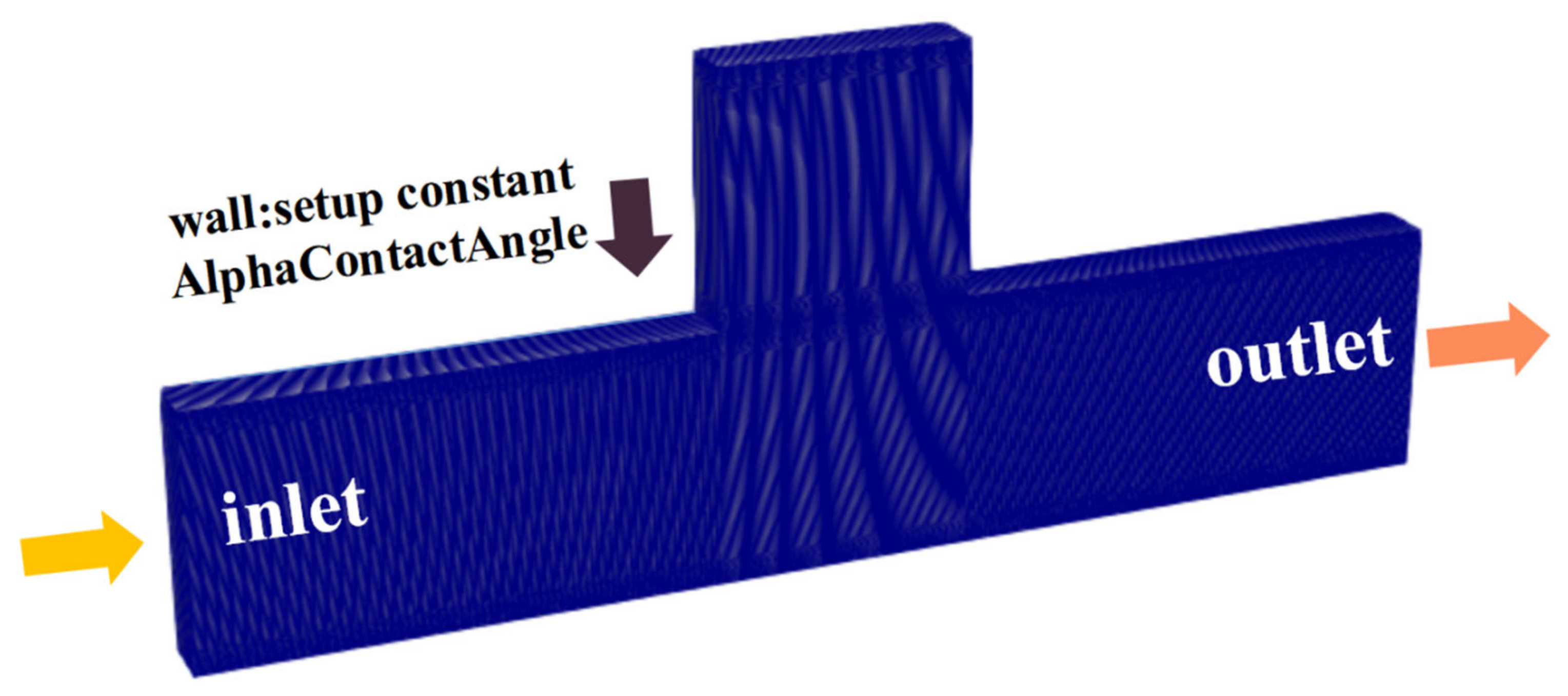
2.1. Physical Model
2.2. Governing Equation of Fluid
2.3. The Constitutive Equation of Viscoelastic Fluid
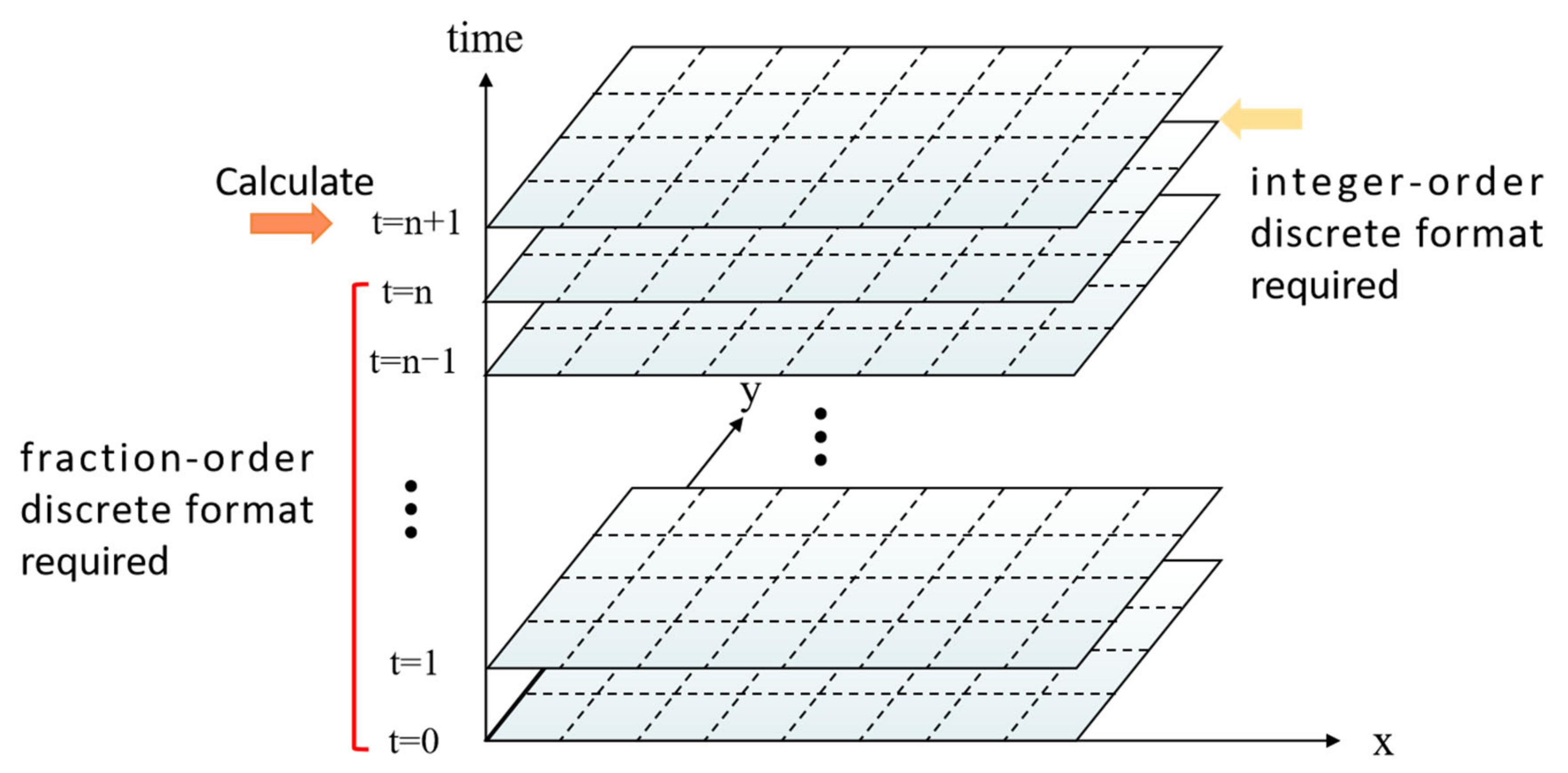
2.4. Numerical Algorithms
- (1)
- The fluid flow in a certain time interval can be regarded as a completely steady state. Therefore, under the physical model we developed in Section 2.1, the strain of the fluid during half the length of the flow through the capillary is assumed to be constant;
- (2)
- Polymers are completely dissolved in water and uniformly distributed in the flow field;
- (3)
- The flow state of the polymer is exactly the same as that of water; i.e., the velocity distribution of both is exactly the same.
3. Result and Analysis
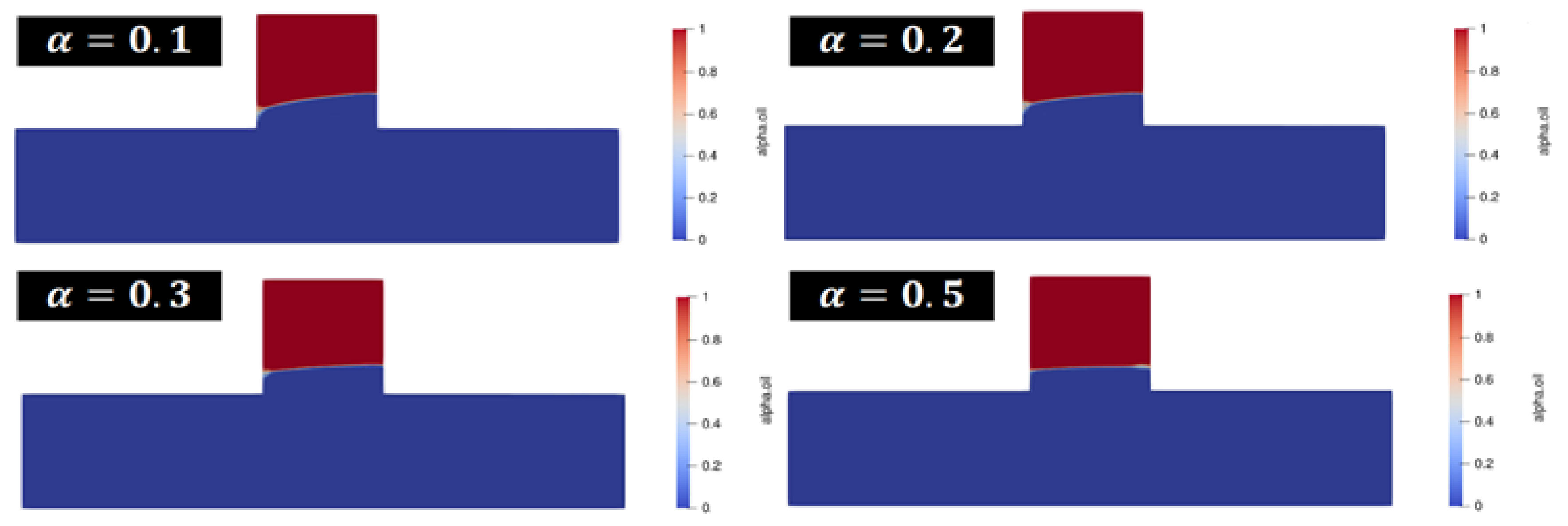
3.1. Effect of on Displacement Efficiency
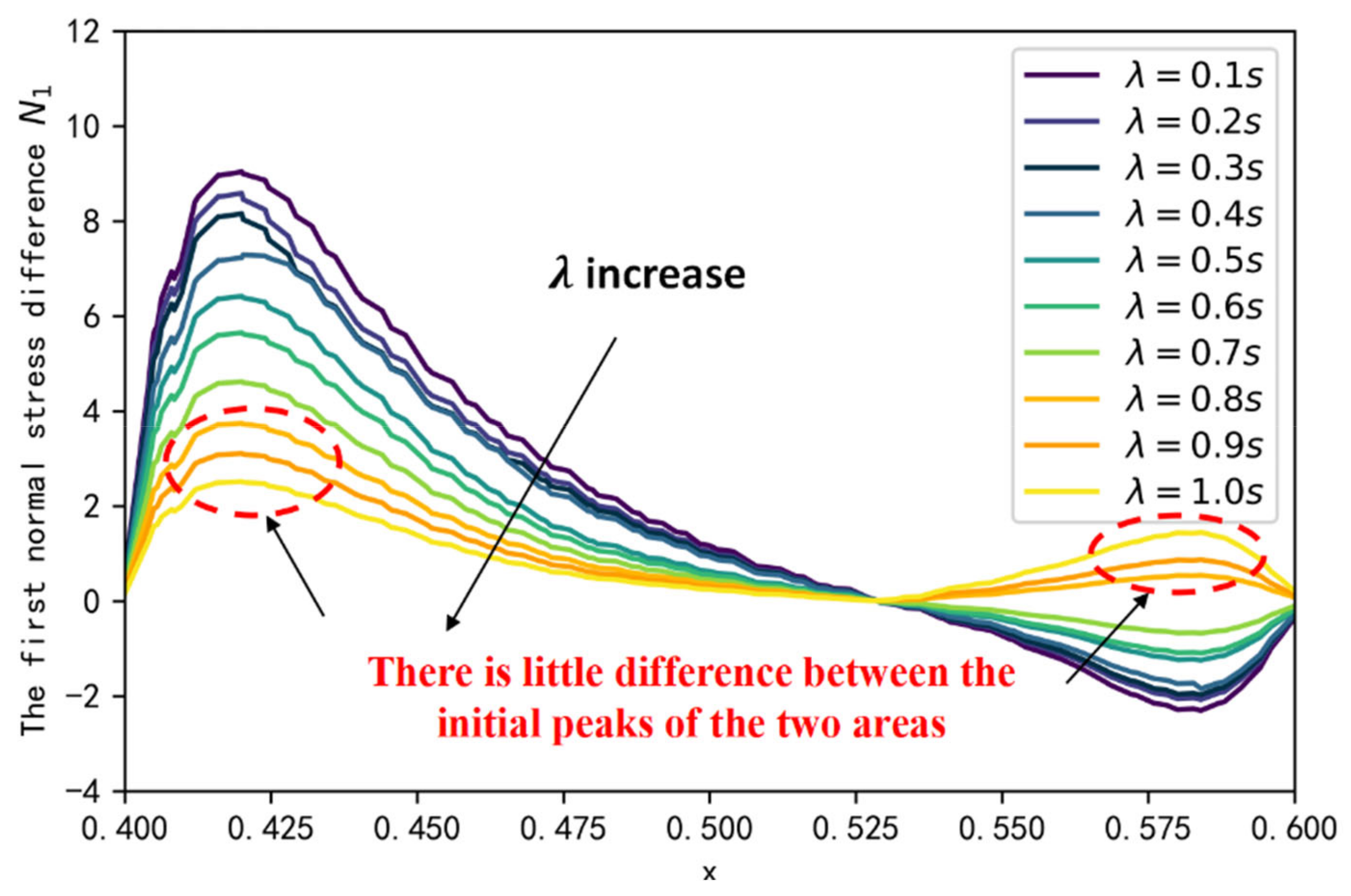
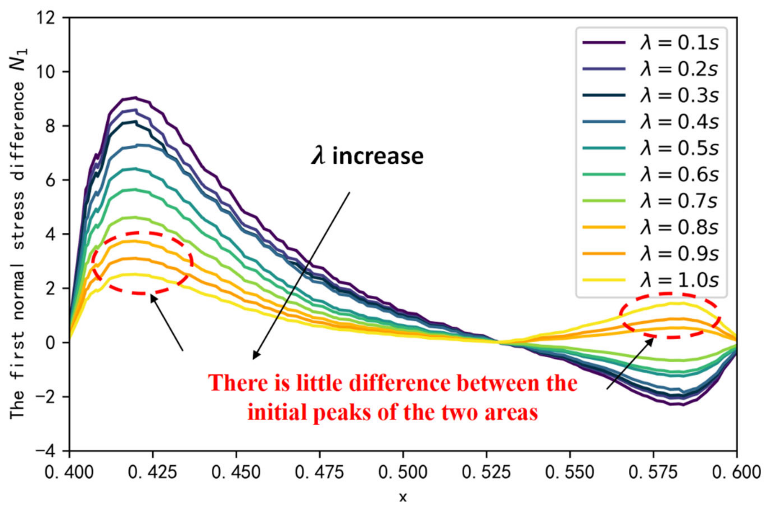
3.2. Effect of on Elastic Perturbation in the Dead End
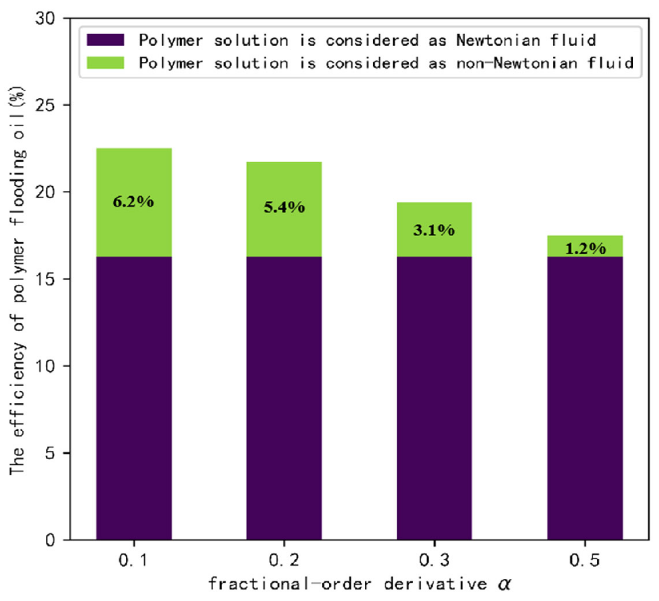
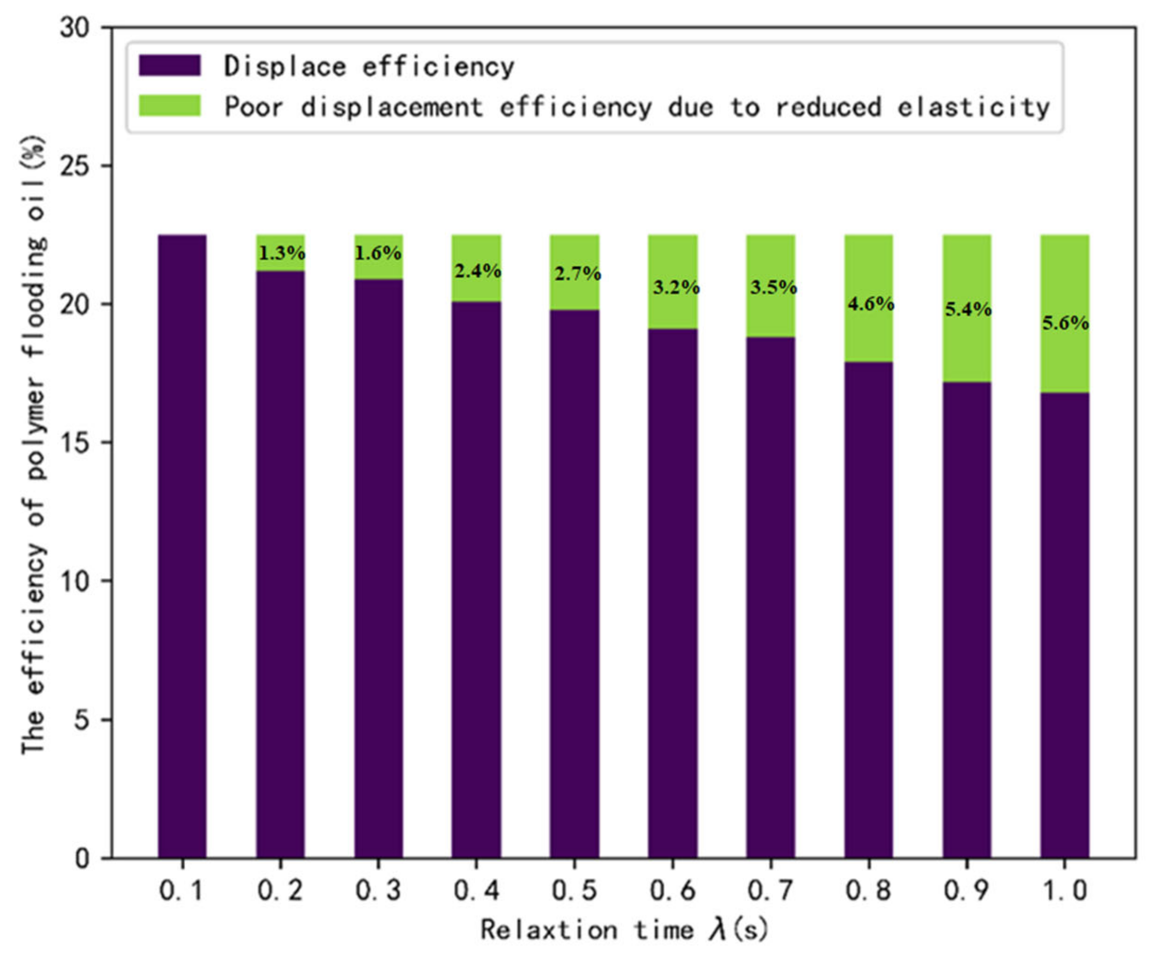
3.3. Effect of on Displacement Efficiency
4. Conclusions
- The viscoelastic fluid is significantly more effective in displacing the remaining oil in the dead end than the Newtonian fluid;
- The perturbed region of viscoelastic fluid within the blind end can be divided into two, which gradually invade deeper into the dead end through the elastic wave transmission between the two areas;
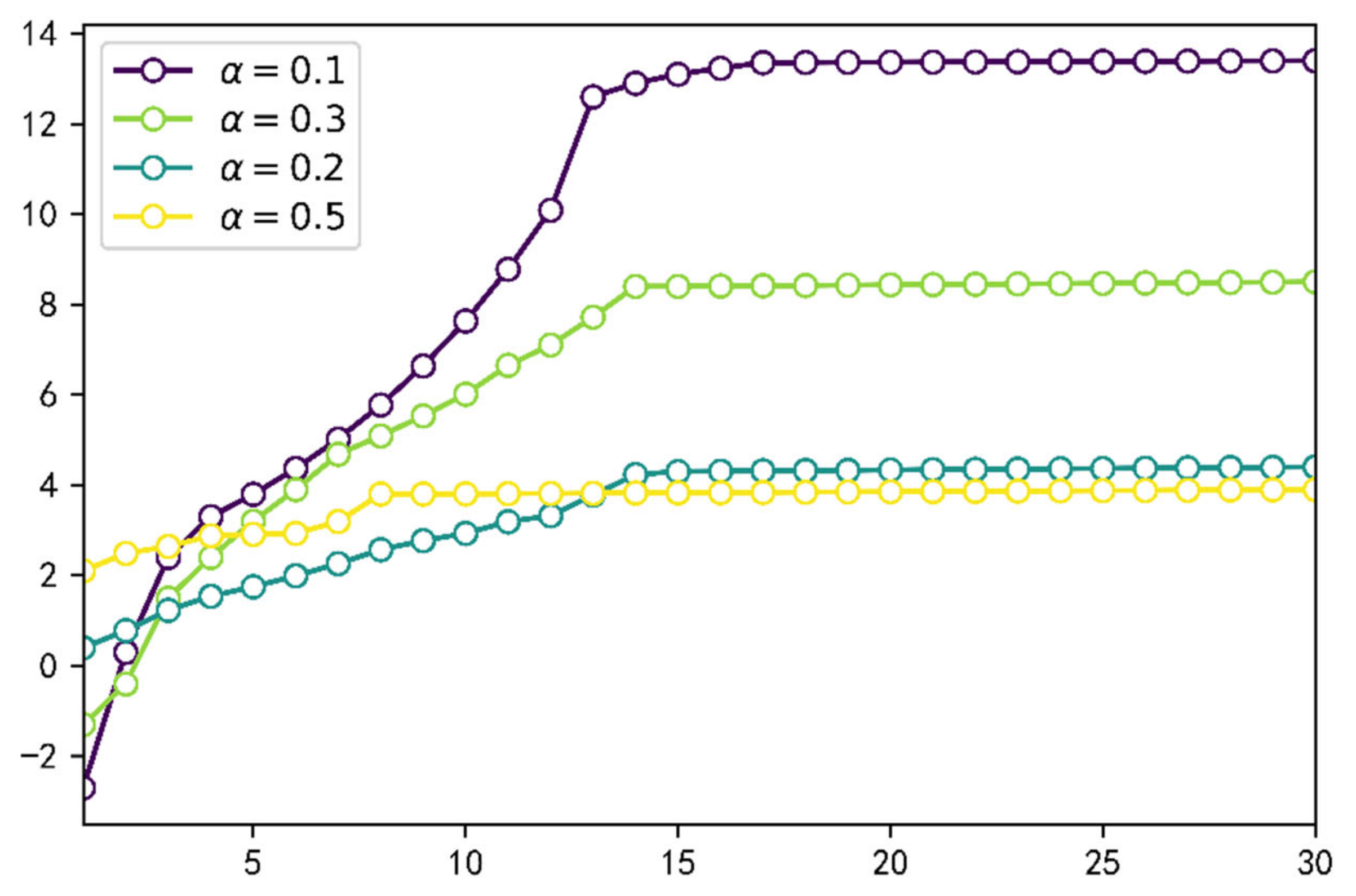
- The smaller the fractional order derivative a, the greater the fluid viscoelasticity and the higher the oil displacement efficiency;
- The smaller the fractional order derivative a, the larger the first normal stress difference peak in the elastic perturbation region 1, the greater the fluid viscoelasticity, and the higher the oil displacement efficiency;
- The relaxation time of the fluid has a significant effect on the viscoelasticity of the fluid, and when the relaxation time is close to 1 s, the flow characteristics of the fluid gradually change from viscoelastic to pure viscous fluid.
Author Contributions
Funding
Conflicts of Interest
References
- Doorwar, S.; Mohanty, K.K. Viscous-fingering function for unstable immiscible flows. SPE J. 2017, 22, 019–031. [Google Scholar] [CrossRef]
- Doorwar, S.; Mohanty, K.K. Extension of the dielectric breakdown model for simulation of viscous fingering at finite viscosity ratios. Phys. Rev. E 2014, 90, 013028. [Google Scholar] [CrossRef] [PubMed] [Green Version]
- Zhang, Y.; Zhao, P.; Cai, M.; Lu, F.; Wu, X.; Guo, Z. Occurrence state and forming mechanism of microscopic remaining oil controlled by dynamic and static factors. J. Pet. Sci. Eng. 2020, 193, 107330. [Google Scholar] [CrossRef]
- Dong, X.; Liu, H.; Chen, Z.; Wu, K.; Lu, N.; Zhang, Q. Enhanced oil recovery techniques for heavy oil and oilsands reservoirs after steam injection. Appl. Energy 2019, 239, 1190–1211. [Google Scholar] [CrossRef]
- Wang, Z.; Liu, Y.; Le, X.; Yu, H. The effects and control of viscosity loss of polymer solution compounded by produced water in oilfield development, International Journal of Oil. Gas Coal Technol. 2014, 7, 298–307. [Google Scholar] [CrossRef]
- Xu, J.; Lu, X. Polymer flood performance and incremental recoveries: Lessons learned from three established cases with varied reservoir heterogeneities. In SPE Asia Pacific Oil & Gas Conference and Exhibition; OnePetro: Richardson, TX, USA, 2020. [Google Scholar]
- Hosseini, S.J.; Foroozesh, J. Experimental study of polymer injection enhanced oil recovery in homogeneous and heterogeneous porous media using glass-type micromodels. J. Pet. Explor. Prod. Technol. 2019, 9, 627–637. [Google Scholar] [CrossRef] [Green Version]
- Seright, R.S. Potential for polymer flooding reservoirs with viscous oils. SPE Reserv. Eval. Eng. 2010, 13, 730–740. [Google Scholar] [CrossRef] [Green Version]
- AlSofi, A.M.; Wang, J.; Kaidar, Z.F. Smartwater synergy with chemical eor: Effects on polymer injectivity, retention and acceleration. J. Pet. Sci. Eng. 2018, 166, 274–282. [Google Scholar] [CrossRef]
- Wang, D.; Cheng, J.; Yang, Q.; Wenchao, G.; Qun, L.; Chen, F. Viscous-elastic polymer can increase microscale displacement efficiency in cores. In SPE Annual Technical Conference and Exhibition; OnePetro: Richardson, TX, USA, 2000. [Google Scholar]
- Wang, D.; Xia, H.; Liu, Z.; Yang, Q. Study of the mechanism of polymer solution with visco- elastic behavior increasing microscopic oil displacement efficiency and the forming of steady oil thread flow channels. In SPE Asia Pacific Oil and Gas Conference and Exhibition; OnePetro: Richardson, TX, USA, 2001. [Google Scholar]
- Xie, K.; Lu, X.; Li, Q.; Jiang, W.; Yu, Q. Analysis of reservoir applicability of hydrophobically associating polymer. SPE J. 2016, 21, 1–9. [Google Scholar] [CrossRef]
- Groisman, A.; Steinberg, V. Efficient mixing at low reynolds numbers using polymer additives. Nature 2001, 410, 905–908. [Google Scholar] [CrossRef] [PubMed]
- Groisman, A.; Steinberg, V. Elastic turbulence in curvilinear flows of polymer solutions. New J. Phys. 2004, 6, 29. [Google Scholar] [CrossRef]
- Poole, R.; Escudier, M. Turbulent flow of viscoelastic liquids through an axisymmetric sudden expansion. J. Non-Newton. Fluid Mech. 2004, 117, 25–46. [Google Scholar] [CrossRef]
- Arratia, P.E.; Thomas, C.; Diorio, J.; Gollub, J.P. Elastic instabilities of polymer solutions in cross-channel flow. Phys. Rev. Lett. 2006, 96, 144502. [Google Scholar] [CrossRef] [PubMed] [Green Version]
- Mitchell, J.; Lyons, K.; Howe, A.M.; Clarke, A. Viscoelastic polymer flows and elastic turbulence in three-dimensional porous structures. Soft Matter 2016, 12, 460–468. [Google Scholar] [CrossRef]
- Howe, A.M.; Clarke, A.; Giernalczyk, D. Flow of concentrated viscoelastic polymer solutions in porous media: Effect of mw and concentration on elastic turbulence onset in various geometries. Soft Matter 2015, 11, 6419–6431. [Google Scholar] [CrossRef]
- Al-Shalabi, E.W.; Ghosh, B. Effect of pore-scale heterogeneity and capillary-viscous finger- ing on commingled waterflood oil recovery in stratified porous media. J. Pet. Eng. 2016, 2016, 708929. [Google Scholar]
- Al-Shalabi, E.W.; Ghosh, B. Flow visualization of fingering phenomenon and its impact on wa- terflood oil recovery. J. Pet. Explor. Prod. Technol. 2018, 8, 217–228. [Google Scholar] [CrossRef] [Green Version]
- Primkulov, B.K.; Pahlavan, A.A.; Fu, X.; Zhao, B.; MacMinn, C.W.; Juanes, R. Signatures of fluid–fluid displacement in porous media: Wettability, patterns and pressures. J. Fluid Mech. 2019, 875, R4. [Google Scholar] [CrossRef] [Green Version]
- Primkulov, B.K.; Talman, S.; Khaleghi, K.; Shokri, A.R.; Chalaturnyk, R.; Zhao, B.; MacMinn, C.W.; Juanes, R. Quasistatic fluid-fluid displacement in porous media: Invasion- percolation through a wetting transition. Phys. Rev. Fluids 2018, 3, 104001. [Google Scholar] [CrossRef]
- Comminal, R.; Spangenberg, J.; Hattel, J.H. Robust simulations of viscoelastic flows at high weissenberg numbers with the streamfunction/log-conformation formulation. J. Non-Newton. Fluid Mech. 2015, 223, 37–61. [Google Scholar] [CrossRef]
- Comminal, R.; Pimenta, F.; Hattel, J.H.; Alves, M.A.; Spangenberg, J. Numerical simulation of the planar extrudate swell of pseudoplastic and viscoelastic fluids with the streamfunction and the vof methods. J. Non-Newton. Fluid Mech. 2018, 252, 1–18. [Google Scholar] [CrossRef]
- Viezel, C.; Tomé, M.F.; Pinho, F.; McKee, S. An oldroyd-b solver for vanishingly small values of the viscosity ratio: Application to unsteady free surface flows. J. Non-Newton. Fluid Mech. 2020, 285, 104338. [Google Scholar] [CrossRef]
- Friedrich, C. Relaxation and retardation functions of the maxwell model with fractional derivatives. Rheol. Acta 1991, 30, 151–158. [Google Scholar] [CrossRef]
- Friedrich, C.; Braun, H. Generalized cole-cole behavior and its rheological relevance. Rheol. Acta 1992, 31, 309–322. [Google Scholar] [CrossRef]
- Song, D.Y.; Jiang, T.Q. Study on the constitutive equation with fractional derivative for the viscoelastic fluids–modified jeffreys model and its application. Rheol. Acta 1998, 37, 512–517. [Google Scholar] [CrossRef]
- Song, D.; Song, X.; Jiang, T.; Lu, Y.; Jiang, D. Study of rheological characterization of fenugreek gum with modified maxwell model. Chin. J. Chem. Eng. 2000, 8, 85–88. [Google Scholar]
- Wenchang, T.; Mingyu, X. Plane surface suddenly set in motion in a viscoelastic fluid with fractional maxwell model. Acta Mech. Sin. 2002, 18, 342–349. [Google Scholar] [CrossRef]
- Khan, M.; Ali, S.H.; Fetecau, C.; Qi, H. Decay of potential vortex for a viscoelastic fluid with fractional maxwell model. Appl. Math. Model. 2009, 33, 2526–2533. [Google Scholar] [CrossRef]
- Zhao, J.; Zheng, L.; Chen, X.; Zhang, X.; Liu, F. Unsteady marangoni convection heat transfer of fractional maxwell fluid with cattaneo heat flux. Appl. Math. Model. 2017, 44, 497–507. [Google Scholar] [CrossRef] [Green Version]
- Sontti, S.G.; Atta, A. Cfd analysis of microfluidic droplet formation in non–newtonian liquid. Chem. Eng. J. 2017, 330, 245–261. [Google Scholar] [CrossRef]
- Brackbill, J.U.; Kothe, D.B.; Zemach, C. A continuum method for modeling surface tension. J. Comput. Phys. 1992, 100, 335–354. [Google Scholar] [CrossRef]
- Weller, H.G. A New Approach to Vof-Based Interface Capturing Methods for Incompressible and Compressible Flow; Report TR/HGW; OpenCFD Ltd.: Bracknell, UK, 2008; Volume 4, p. 35. [Google Scholar]
- Wang, B.-X.; Zhou, L.-P.; Peng, X.-F. A fractal model for predicting the effective thermal conductivity of liquid with suspension of nanoparticles. Int. J. Heat Mass Transf. 2003, 46, 2665–2672. [Google Scholar] [CrossRef]
- Metzler, R.; Klafter, J. The random walk’s guide to anomalous diffusion: A fractional dynamics approach. Phys. Rep. 2000, 339, 1–77. [Google Scholar] [CrossRef]
- Lynch, V.E.; Carreras, B.A.; del Castillo-Negrete, D.; Ferreira-Mejias, K.; Hicks, H. Numerical methods for the solution of partial differential equations of fractional order. J. Comput. Phys. 2003, 192, 406–421. [Google Scholar] [CrossRef]
- Jasak, H. Error Analysis and Estimation for the Finite Volume Method with Applications to Fluid Flows. Ph.D. Thesis, University of London, London, UK, 1996. [Google Scholar]


| Oil | Displacement Fluid () | |||
|---|---|---|---|---|
| Water | Polymer () | |||
| Density (kg/m3) | 860 | 1000 | 1000 | |
| Viscosity (mPa·s) | 9 | 1 | 4 × 10⁴ | |
| Interfacial tenso (mN/m) | 5 | |||
Publisher’s Note: MDPI stays neutral with regard to jurisdictional claims in published maps and institutional affiliations. |
© 2022 by the authors. Licensee MDPI, Basel, Switzerland. This article is an open access article distributed under the terms and conditions of the Creative Commons Attribution (CC BY) license (https://creativecommons.org/licenses/by/4.0/).
Share and Cite
Huang, J.; Chen, L.; Li, S.; Guo, J.; Li, Y. Numerical Study for the Performance of Viscoelastic Fluids on Displacing Oil Based on the Fractional-Order Maxwell Model. Polymers 2022, 14, 5381. https://doi.org/10.3390/polym14245381
Huang J, Chen L, Li S, Guo J, Li Y. Numerical Study for the Performance of Viscoelastic Fluids on Displacing Oil Based on the Fractional-Order Maxwell Model. Polymers. 2022; 14(24):5381. https://doi.org/10.3390/polym14245381
Chicago/Turabian StyleHuang, Jingting, Liqiong Chen, Shuxuan Li, Jinghang Guo, and Yuanyuan Li. 2022. "Numerical Study for the Performance of Viscoelastic Fluids on Displacing Oil Based on the Fractional-Order Maxwell Model" Polymers 14, no. 24: 5381. https://doi.org/10.3390/polym14245381