Abstract
This work focuses on the mathematical analysis of the controlled release of a standardized extract of A. chica from chitosan/alginate (C/A) membranes, which can be used for the treatment of skin lesions. Four different types of C/A membranes were tested: a dense membrane (CA), a dense and flexible membrane (CAS), a porous membrane (CAP) and a porous and flexible membrane (CAPS). The Arrabidae chica extract release profiles were obtained experimentally in vitro using PBS at 37 °C and pH 7. Experimental data of release kinetics were analyzed using five classical models from the literature: Zero Order, First Order, Higuchi, Korsmeyer–Peppas and Weibull functions. Results for the Korsmeyer–Peppas model showed that the release of A. chica extract from four membrane formulations was by a diffusion through a partially swollen matrix and through a water filled network mesh; however, the Weibull model suggested that non-porous membranes (CA and CAS) had fractal geometry and that porous membranes (CAP and CAPS) have highly disorganized structures. Nevertheless, by applying an explicit optimization method that employs a cost function to determine the model parameters that best fit to experimental data, the results indicated that the Weibull model showed the best simulation for the release profiles from the four membranes: CA, CAS and CAP presented Fickian diffusion through a polymeric matrix of fractal geometry, and only the CAPS membrane showed a highly disordered matrix. The use of this cost function optimization had the significant advantage of higher fitting sensitivity.
1. Introduction
Arrabidaea chica Verlot is a type of shrub found in tropical America, from the south of Mexico to Brazil, being very common in the Amazon rainforest [1]. As the extract of A. chica is an important source of tannins, flavonoids and anthocyanins, it presents different medicinal properties, such as antioxidant, antiseptic, anti-inflammatory and antifungal activities [2]. One of its main components is the anthocyanin ‘carajurina’, which can be used as a marker for the detection and quantification of the extract of A. chica.
One of the strategies to deliver drugs and other medicinal substances is through controlled release systems, which maintain the drug concentration in the blood or in target tissues as long as possible at a desired value, being able to control the drug release rate and duration [3]. Different biopolymers have been used to deliver drugs and other compounds for the treatment of skin lesions in a local, targeted and controlled manner [4]. One of the most versatile biopolymers is chitosan, which is obtained mainly from shells of crustaceans, such as shrimp [5]. In this regard, Servat-Medina et al. (2015) [6] synthesized chitosan nanoparticles loaded with different concentrations of A. chica extract (10 to 25% relative to chitosan mass) for the treatment of skin ulcers. Recently, in 2020, our group reported synthesizing different types of chitosan/alginate (C/A) membranes to be used as controlled release systems of A. chica extract, as an alternative for the treatment of skin lesions [7]. C/A membranes are attractive because they are insoluble in water, stable to pH variations and capable of incorporating different bioactive agents into their matrix.
Mathematical modeling of drug delivery and predictability of drug release has been a field of academic and industrial importance for several decades [8]. In 1961, Higuchi published his famous equation allowing for a surprisingly simple description of the drug release mechanism from an ointment base. Numerous models have been proposed since then, including empirical/semi-empirical as well as mechanistic realistic ones [9]. Consequently, many different mathematical approaches have been proposed to assess the similarity between drug dissolution and mass transfer profiles [10].
A versatile mathematical tool is the cost function analysis, which is an optimization process that consists of measuring the difference between real experimental data with the prediction of a model. The objective of this analysis is to minimize this difference, that is, to find the parameters that allow the model to fit the data as closely as possible [11]. The cost function can be performed for any type of mathematical model and compared with various experimental data; regarding numerical optimization methods, local gradient methods such as conjugate gradients [12,13] or global parameter population methods such as genetic algorithms [11,14] or deep learning strategies [15] can be applied.
The method in this work focuses on the quantitative assessment of the controlled release of a standardized extract of A. chica from C/A membranes. First, in vitro experimental A. chica kinetic release profiles were obtained from four different formulations of C/A membranes: a dense membrane (CA), a dense and flexible membrane (CAS), a porous membrane (CAP), and a porous and flexible membrane (CAPS). Later, the mechanisms of the extract release kinetics were determined comparing the coefficient obtained using five classic models from the literature [16]: Zero Order, First Order, Higuchi, Korsmeyer–Peppas and Weibull model functions. Finally, as the main novelty of this work, the release profiles were analyzed using an optimization method implemented by our group that employs the cost function approach to determine the model parameters that best fit to the experimental data.
2. Materials and Methods
2.1. Materials
Chitosan (C, from shrimp shells 96% deacetylated and g/mol), medium viscosity sodium alginate (A, from Macrocystis pyrifera g/mol), Kolliphor P188 (a pore-forming surfactant) and phosphate buffer solution (PBS) 0.01 M (0.138 M NaCl, 0.0027 M KCl, pH = 7.4) were acquired from Sigma-Aldrich (Sao Paulo, Brazil). Silpuran 2130 A/B (a silicone polymer) was obtained from Wacker Chemie AG (Munich, Germany), and glacial acetic acid, calcium chloride dihydrate and sodium salt from Merck KGaA (Sao Paulo, Brazil). The standardized Arrabidaea chica Verlot extract was supplied by the Division of Chemistry of Natural Products of the Center for Chemical, Biological and Agricultural Research (CPQBA) at the University of Campinas (Campinas, Brazil). The used water was deionized in a Milli-Q System from Millipore.
2.2. Membranes synthesis
Four formulations of C/A membranes containing A. chica extract (10% in weight) were obtained according to the protocol previously described by Pires et al. (2020) [7]. The main synthesis differences are summarized as follows: (A) CA membrane: prepared with chitosan 1% (m/v) in acetic acid 2% and alginate 0.5% (C:A = 1:2 v/v); (B) CAS membrane: synthesized with the same CA formulation, but including 10% of Silpuran 2130 A/B; (C) CAP membrane: obtained by formulating CA membrane plus 10% in weight of the Kolliphor P188; (D) CAPS membrane: It was synthesized by formulating CAS plus 10% in weight of Kolliphor P188. In all cases, the membranes were cross-linked with calcium ions.
2.3. Morphology of the Membranes
Membrane samples containing the A. chica extract were microscopically observed and photographed using a Nikon digital camera (COOLPIX model S3300). The cross section morphology of the membranes was analyzed using a scanning electron microscope (model Leo 440i, Leica). Samples of were fixed on a suitable support and metalized (mini-Sputter coater, SC 7620) by depositing a thin layer of gold (92 Å) on their surfaces.
2.4. Release Experiments
To obtain the release profiles, membrane samples (2 cm × 2 cm) containing the A. chica extract were previously weighed and immersed in a 10 mL of PBS solution containing 20% ethanol at pH 7.4, C and 100 rpm. At predetermined time intervals up to 48 h, 1 mL of the solution was withdrawn for absorbance analysis using a spectrophotometer (Thermo Scientific Evolution–220, Thermo Fisher Scientific, Waltham, MA, USA) at 470 nm and then returned to the vial. The analytical curve was prepared using A. chica extract also dissolved in a PBS solution containing 20% ethanol. All experiments were performed in triplicate, and mean values were used. Sink conditions were maintained during the drug release experiments and at predetermined time intervals, the supernatant solution was completely renewed.
2.5. Mathematical Models
The mechanism of drug release was determined by fitting the mathematical models to the experimental data using OriginPro 8.5 software. Five models were studied, the main characteristics of which are outlined below [17,18,19,20].
In the zero-order model, the drug is released at a constant rate independent of concentration, and dissolution from dosage forms that do not disaggregate and release the drug slowly. This model is represented by the equation
where is the amount of drug released at time t, is the initial amount of the extract in the solution and is the zero-order proportional constant.
In the first-order model, the release is a concentration-dependent process, and the equation that gives the release behavior is
where and are again the amount of drug released at time t and the initial amount of the extract in the solution, respectively, and is the first-order release kinetic constant.
The Higuchi model implies more assumptions, such as that the initial drug concentration in the matrix is higher than drug solubility; drug diffusion takes place only in one dimension (edge effect must be negligible); drug particles are smaller than system thickness; matrix swelling and dissolution are negligible; drug diffusivity is constant; and perfect sink conditions are always attained in the release environment. The general release equation is given by
where is the amount of drug released in time t per unit area, and is the Higuchi dissolution constant. It represents a Fickian diffusion of drugs without the matrix dissolution taken into account.
The Korsmeyer–Peppas model is a simple relationship to describe drug release from a polymeric system. This semi-empirical model analyzes both Fickian and non-Fickian release of drug from swelling as well as non-swelling materials; however, it is applied just up to 60% of the drug amount released. The Korsmeyer–Peppas release equation is given by
where the ratio is the fraction of drug released at time t, is the Korsmeyer–Peppas kinetic constant, which characterizes the drug–matrix system and n is the exponent that indicates the drug release mechanism.
The Weibull model is an alternative description for the dissolution and release processes, and can be applied for most types of dissolution curves. The Weibull equation expresses the cumulative fraction of the drug, , in a solution at time t, by the following expression:
where is related to the specific surface of the dosage matrix form, is mainly related to the mass transport characteristics of the device and represents the delay time before starting the dissolution or release process, which in most cases is 0.
3. Cost function Analysis
3.1. Definition of Cost Function
We introduce the notation for a general model that depends on the parameter vector . For example, for the Korsmeyer–Peppas model, the parameter set is specified as
A standard technique that enables the interpretation of experimental data with a quantitative model is the formulation as an inverse problem, where the direct problem is formulated as a mathematical model, such that the distance of the model to the data
is described by a cost function [11,21]
where accounts for different metrics of the distance between model and data, and contains weights of the data points. For (in comparison to ), we have an underestimation respective overestimation of the measurement errors (under the assumption that the model is correct) for small respective high distances between data and model. Though, applies the concept of least squares, which is more common, in spite of the bias.
Regarding the weights, there are various choices, as the following prototypes, among which there are multiple possible variants:
- Equal weights for all i.
- Switch off at a threshold time ,
- Adaptive weights, that gives higher emphasis to smaller times, such as, for example,
The switch off in case (2) at a threshold time applies, i.e., should apply, for model approximations that do not satisfy asymptotic upper limits, such as the models of Higuchi or Korsmeyer–Peppas, which are designed to be valid for lower times only. As their unlimited asymptotic behavior is qualitatively wrong, above a threshold value the models are quantitatively wrong. In favor of the Higuchi and Korsmeyer–Peppas models, the weighting choice was case (2) with data switch off at h. For the Weibull model we choose case (1).
The inverse problem is solved by minimizing the cost function,
that gives the optimal set of parameters . The mathematical model can have the form of differential equations that in turn include parametric functions, or the mathematical model is expressed directly in terms of parametric functions. For the minimization of the cost function, an issue might be (1) high correlations between the parameters, or (2) its non-convexity. In the case of high parameter correlation that touch the scale of computational errors induced by the machine error, even the optimal numerical method cannot compensate a wrong model choice; it is an issue of model choice. In the case of non-convexity of the cost function, the optimization method needs to be chosen carefully, or the experimentation with different optimization methods is subject of research, e.g., global optimization methods, where populations of parameter sets are optimized, instead of local methods with only one single parameter set.
3.2. Cost Function Minimization: Optimality Conditions
The goal is to minimize the cost function, that is, to find the parameters of each model that fits the experimental data as closely as possible.
As a criterion of optimality [22], there is a necessary condition and a sufficient condition. For two-variable models, the necessary condition for optimality is that the gradient is equal to zero in each of its components,
The sufficient condition of optimality is that the Hessian matrix
is positive definite for a minimum, i.e., according to the definition
This definition can be written as
A general criterion of a square matrix of any size to be positive definite is that all eigenvalues are positive.
3.3. Equivalence of Optimization Methods
The comparison of model predictions with data,
defines a residual function , where we want to find its zeros, which can only be calculated approximately if the system is overdetermined. An approximation criterion is the sum of squares
which is equivalent to the cost function (6), but for the specific choice of and with equal weights, i.e. case (1).
There are two different paths to obtain optimal parameters:
An iterative procedure that solves an overdetermined system of nonlinear equations, such as (6) is the Gauss–Newton algorithm. This means that an initial estimate of the vector parameter must be provided.
4. Methodology: Implementation
The five mathematical models of Section 2.5 were tested in parallel. The generated process was automated by subroutines (see Supplementary Materials).
Prior to the calculations, the derivatives and the gradients were obtained for one- and two-variable models, respectively, in order to verify the fulfillment of the necessary condition. The sufficient condition was satisfied, as for one-variable models the second derivative, and for two-variable models the elements in the Hessian matrix were different from zero.
In the implementation, the corresponding equations and the experimental data were consistent enough to be called by the common cost function subroutine.
The algorithm for the cost function is given in the Algorithm S1 (see Supplementary Materials for Algorithms). The following criterion has to be satisfied:
where c is the cost function, N is the number of experiments for each membrane in a given time t (in our case ) and J is the number of data in the experiment. A syntax was chosen from the model subroutine (Algorithm S2):
where the vector of variables consisted of the observation times, to calculate the solution of the model at given times. The description of steps to implement this methodology is presented in Algorithm S4.
It is important to consider that a better fit is expected with the cost function used in models with several parameters. However, that does not necessarily mean that the type of model as such is better or that it effectively better explains the phenomenon. Moreover, a higher number of parameters causes optimization algorithms to have problems when approaching the ‘optimal’ data, given the higher correlation within the same parameters.
5. Results and Discussion
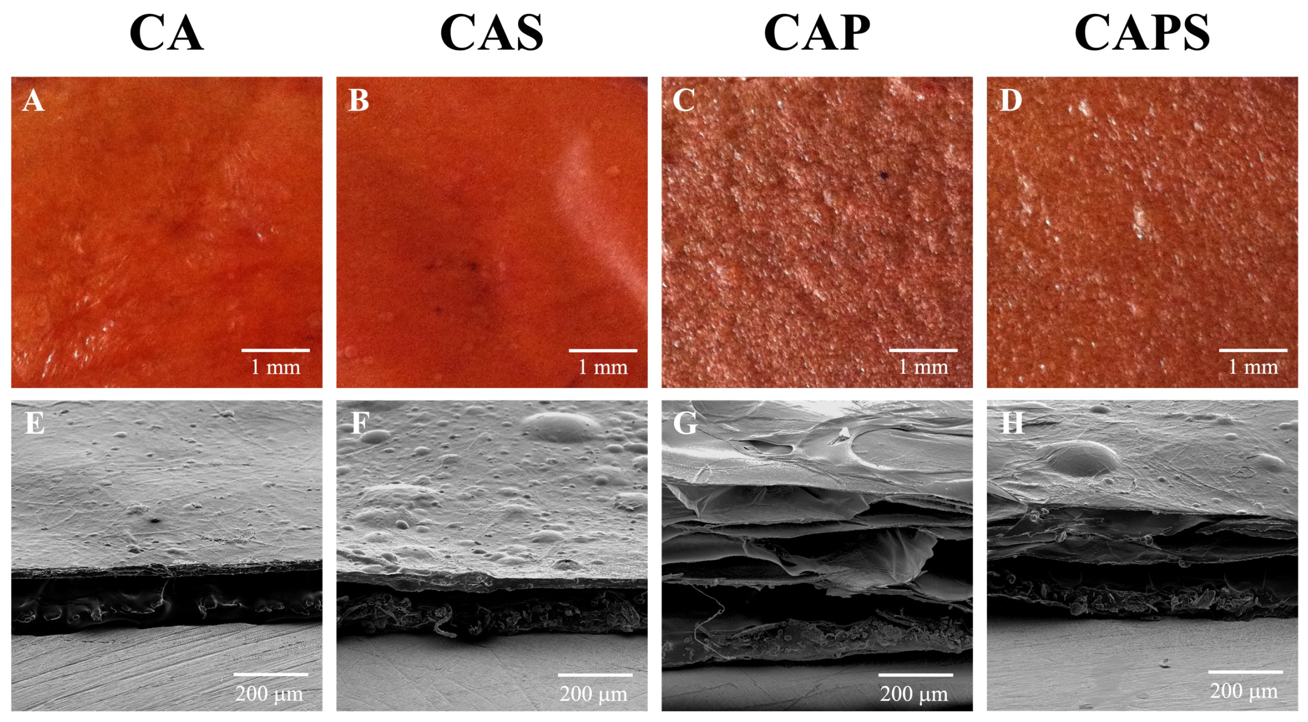
The obtained membranes presented the geometrical form of a thin slab. Figure 1 shows photographs and SEM images of the membrane samples loaded with A. chica extract. The observed intense red color in the photographs (Figure 1A–D) was due to the insoluble anthocyanin pigments carajurin and carajurone included in the A. chica extract [23]. The membranes produced without Kolliphor P188 surfactant turned out to be dense and compact (CA and CAS). However, for the formulations synthesized using the surfactant, the membranes were porous and thicker (CAP and CAPS). When the silicone Silpuran 2130 was included in the formulation, samples were soft and flexible to the touch (CAS and CAPS). In summary, the general characteristics of the obtained membranes were as follows: CA was dense, thin and rigid; CAS was dense, thin but flexible due to the silicone; CAP was rigid but thick and porous due to air bubbles in its matrix generated by the surfactant; and CAPS was thick and porous due to the surfactant, but flexible because of the silicone.

Figure 1.
Photographs and SEM images of membrane samples loaded with A. chica extract: CA (A,E), CAS (B,F), CAP (C,G) and CAPS (D,H).
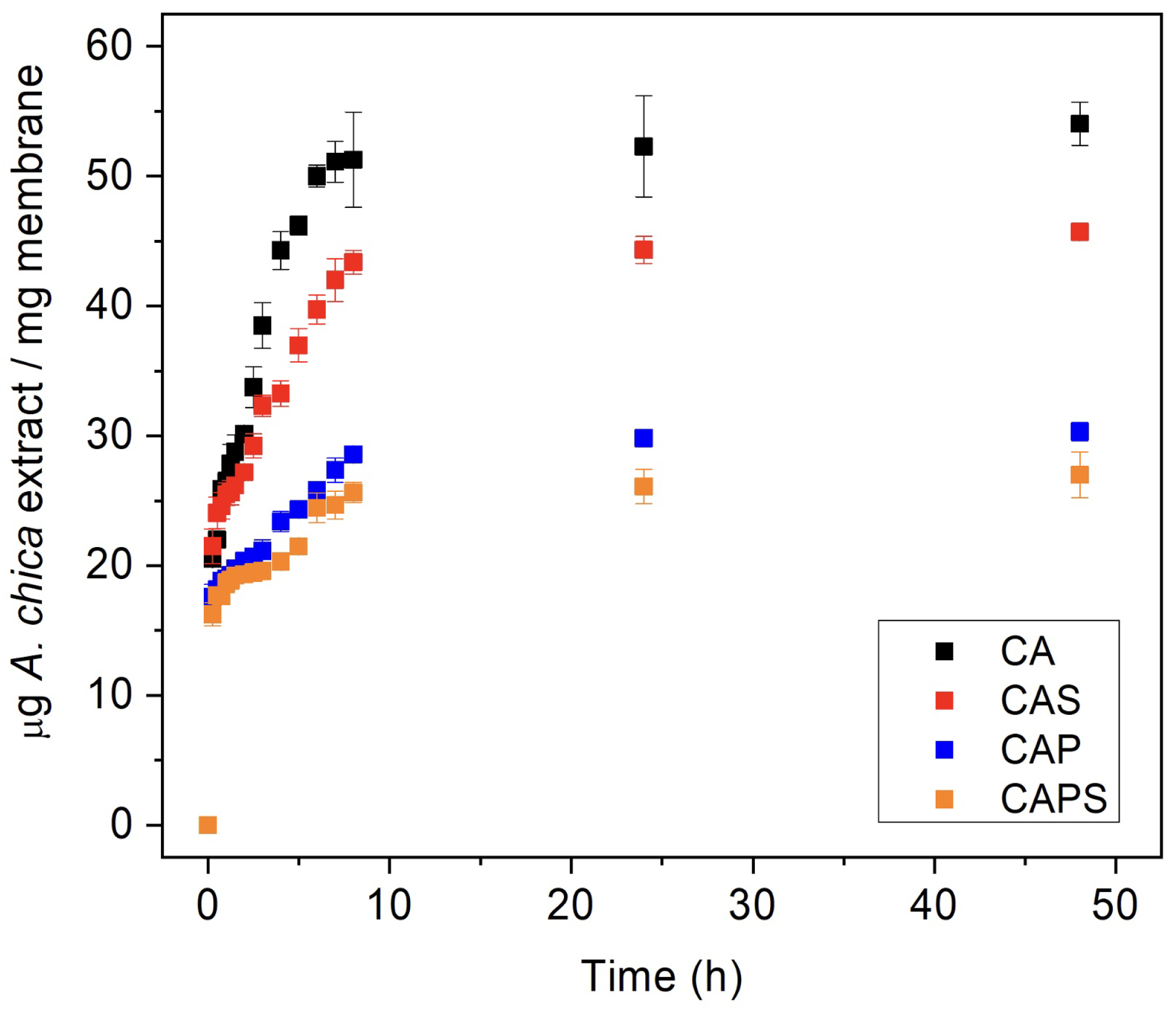
A. chica extract release profiles are shown in Figure 2. Although all samples were loaded with the same percentage of extract (10% in weight), CA and CAS membranes released higher amounts of extract per mass of polymer than CAP and CAPS. The burst release observed in the first minutes of the process can be attributed to the fraction of the drug which is adsorbed or weakly bound to the surface area of the polymer rather than to the drug incorporated into the polymer matrix [24]. Moreover, the lower amounts in porous formulations can be explained by the higher dispersion of the mixture due to the presence of the surfactant with a consequent increase in the interphases of the extract with the polymers. For all cases, the maximum amount of extract released was reached at 24 h. Re-absorption of the extract by the membranes was not observed because the maximum released values of extract were maintained constant for up to 48 h.

Figure 2.
Experimental A. chica extract release profiles from the C/A membranes. Results represent mean ± SD of three measurements.
To gain a deeper insight into the mechanisms that govern the release of A. chica extract from the membranes, five mathematical models were fitted to the experimental data: Zero-order, First order, Higuchi, Korsmeyer–Peppas and Weibull. Experimental data were normalized and only evaluated up to 8 h because these models are semi-empiric and better valid for the first stages of release; as mentioned previously in Section 3.1, where the weights on the cost function switch off (7) at a threshold value of time .
The switch off is an artificial fix for a model that is valid for short time intervals and loses pertinence at bigger times. In order to avoid this artificial switch off, one can select admissible functions for a semi-empirical model that satisfy physically reasonable criteria. For the drug release model, these characteristics should address at least the following components:
- Zero release at zero time.
- Increasing cumulative release for advancing time.
- Existence of an upper bound for the total release at sufficiently long period.
These characteristics can be expressed as
With help of these model design indications, we can assess the various models (see Table 1 for a qualitative model comparison).

Table 1.
Model evaluation: Satisfaction status of criteria by considered models.
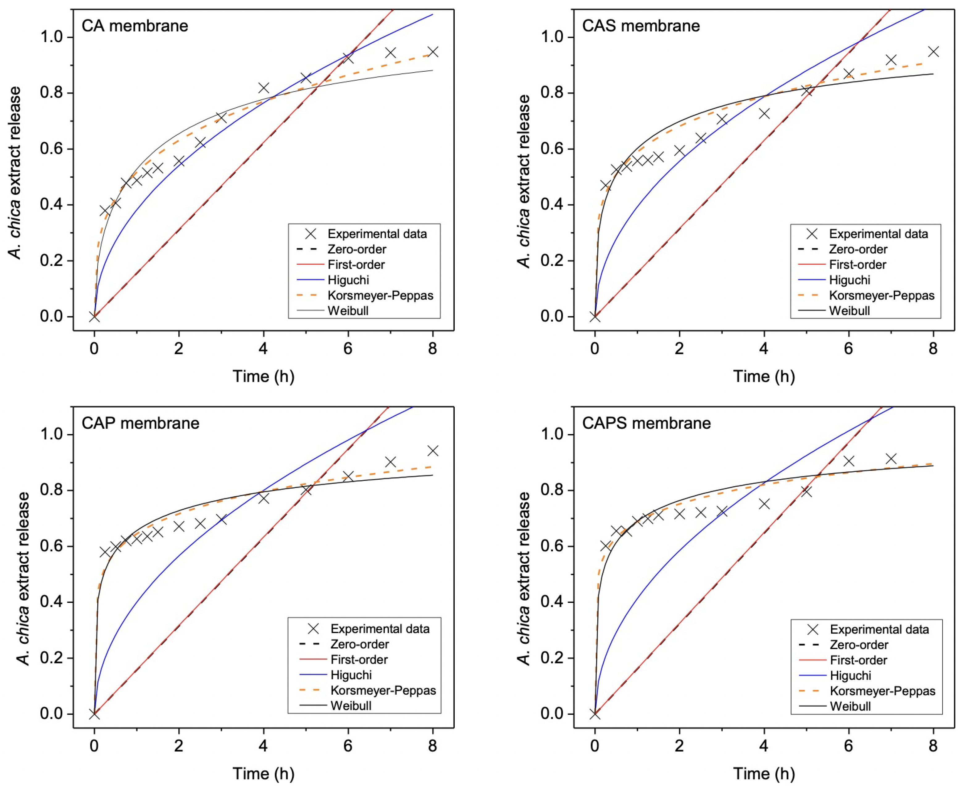
Simulations of the release profiles from each membrane using the indicated models are shown in Figure 3. From these simulations, the kinetic parameters were extracted and presented in Table 2. The coefficient (coefficient of determination) was used to compare the results between models. The value of is usually between 0 and 1, and generally a higher value means that the model fits the data better; some equal to or higher than 0.95 is considered as a good fitting by linear regression. Therefore, according to the values generated by each model (Zero-order, First-order, Higuchi, Korsmeyer–Peppas and Weibull) for each membrane (CA, CAP, CAPS and CAPS), the models that best fit the release profiles were Korsmeyer–Peppas and Weibull. In the case of the Korsmeyer–Peppas model, values of all samples were higher than 0.95, but in the case of the Weibull model, the fitting for the CA and CAP membranes returned values of almost 0.95 and for the CAS and CAPS membranes, values were higher than 0.95.
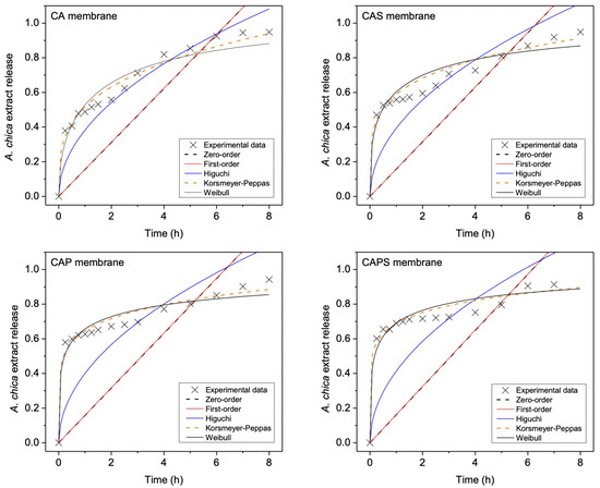
Figure 3.
Simulations of the release profiles from each membrane (CA, CAS, CAP and CAPS) using the Zero-order, First-order, Higuchi and Korsmeyer–Peppas and Weibull models.
Table 2.
In vitro release kinetics of A. chica from C/A membranes.
Korsmeyer–Peppas is a model determined on the basis of experimental data and it is a shortened version of the solution of the diffusion equation by Crank (1975) [25]. In this model, the release mechanisms are dependent on the sample geometry (thin films, cylinders, spheres). In that sense, when the Korsmeyer–Peppas model is applied to thin films, such as the membranes of this study, if the release parameter n is less than 0.5, it means that drug diffusion is occurring through a partially swollen matrix and through a solution-filled network mesh [26]. If , the Fickian diffusion is controlling the release and the solvent penetration is the rate-limiting step. On the other hand, if , then this is related to a non-Fickian release, which is the release of the extract controlled by both diffusion and erosion mechanisms. If , then the release corresponds to the zero-order model, where the release of the extract is independent of time [9]. In that sense, according to the results from the Korsmeyer–Peppas model, the n values for the four types of membranes were lower than 0.5; this indicates that the release of the extract was controlled by a diffusion occurring through a partially swollen matrix, which could be produced by the polymer chains relaxation. Moreover, the parameter is related to the interaction between the extract and the constituent polymers of the membrane, and higher values mean higher rates of release. According to this, the values obtained for the samples presented the following tendency:
CAPS > CAP > CAS > CA.
This means that the porous membranes (CAPS and CAP) generated a faster release probably due to the pores of the polymeric matrix, which facilitated the absorption of water from the release medium (PBS). On the contrary, for membranes without pores (CAS and CA), which are more compact and dense, the absorption of water would be limited, and as a consequence, the release of the extract, too. As CAS and CA samples obtained higher amounts of extract release than CAPS and CAP (Figure 2), this means that faster release of CAPS and CAP was mainly controlled by the porous membrane cross-linked structure rather than the concentration differential. On the other hand, although the Weibull model has been criticized for the lack of a kinetic basis for its use and for the non-physical nature of its parameters, according to different works, the Weibull function demonstrated that the exponent , for polymeric matrices, is an indicator of the mechanism of transport of the drug through the matrix related to the exponent n of the power law model [17,27,28,29]: a value of less than or equal to 0.75 was associated with Fick diffusion in either fractal or Euclidean space, while a combined mechanism (Fick diffusion and swelling controlled transport) was associated with values in the range 0.75 < < 1. For > 1, drug release involves complex mechanisms, which imply that the release rate does not change monotonically. In fact, the release rate initially increases nonlinearly up to an inflection point and then decreases asymptotically.
According to the above, the results obtained for the Weibull parameter (Table 2) indicated that the mechanism of release was Fickian diffusion ( less than or equal to 0.75). However, it is also important to identify the polymeric matrix geometry in this range [27]: for < 0.35, diffusion occurs in highly disordered spaces, differently than the percolation cluster; for , diffusion occurs in a fractal substrate; for , diffusion takes place in a normal Euclidean space. These results suggest that the non-porous membranes (CA and CAS) present a fractal structure, and the porous formulations (CAP and CAPS) show highly disordered structures. Fractal organization of CA and CAS samples could be originated during the association of alginate carboxylic groups (-COO) with chitosan amino groups (-NH3) [7,30]; meanwhile, the polymeric matrices of CAP and CAPS were highly disorganized by the pores formation.
As a summary, the release of A. chica extract from all membrane formulations occurred by a Fickian difussion, what was confirmed by both Korsmeyer–Peppas and Weibull models. Moreover, the Weibull model suggested that non-porous membranes (CA and CAS) had fractal geometry and that porous membranes (CAP and CAPS) were highly disorganized structures.
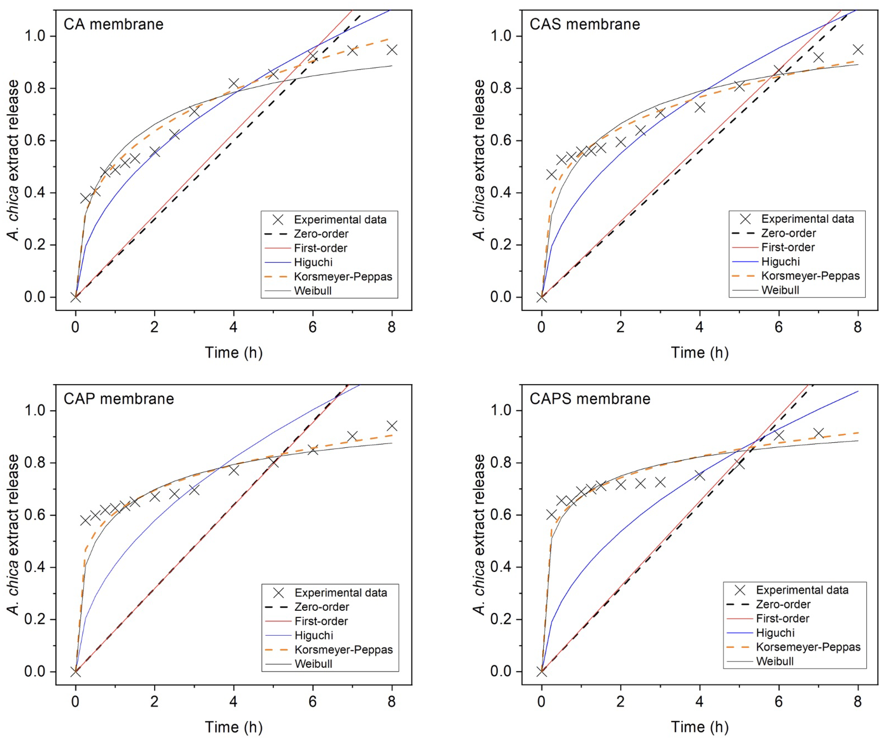
Furthermore, in this work, the cost function is presented as a tool to analyze different mathematical models that simulate experimental data of release profiles of A. chica extract from C/A membranes to a greater extent. Accordingly, Figure 4 shows the cost function simulations applied to each model (Zero-order, First-order, Higuchi, Korsmeyer–Peppas and Weibull) in each membrane type (CA, CAS, CAP and CAPS), and Table 3 presents the parameters obtained. The lower the fitted cost function value (F), the more efficient the model. Conversely, when the cost function value is higher, the model is less effective.
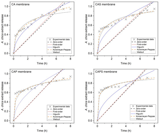
Figure 4.
Cost function simulations of the mathematical models (Zero-order, First-order, Higuchi and Korsmeyer–Peppas and Weibull) used in each membrane: CA, CAS, CAP and CAPS.
Table 3.
Summary of results of the cost function fitting.
According to the results obtained by the cost function, F values in Table 3, the best simulations were performed by
which is similar to the previous results. However, it is important to highlight that using the cost function, the Weibull model fits better to the release profiles than the Korsmeyer-Peppas model for all the membranes. Note that in the case of the Weibull model and correspond to and , respectively, and the value, which is , was not reported because it is zero for all cases (Table 2). According to the cost function results, CA, CAS and CAP formulations would present a Fickian diffusion through a polymeric matrix of fractal geometry, and only the CAPS membrane would have a highly disordered matrix. This partially different result compared to the case when the cost function is not applied can be due to the fact that F values of the Weibull model are around 10 times lower—i.e., 10 times mores precise—than the Korsmeyer–Peppas model. Without the use of the cost function, the of both models are very similar. In that sense, the cost function presents a significant advantage, which is a higher fitting sensitivity.
Weibull > Korsmeyer–Peppas >
> Higuchi > First-order > Zero-order,
> Higuchi > First-order > Zero-order,
6. Conclusions
This work consisted on studying the performance of in vitro experimental A. chica extract release profiles obtained from four different formulations of chitosan/alginate membranes: a dense membrane (CA), a dense and flexible membrane (CAS), a porous membrane (CAP), and a porous and flexible membrane (CAPS). The mechanism of the extract release kinetics was determined comparing classic models from the literature: Zero Order, First Order, Higuchi, Korsmeyer–Peppas and Weibull. Furthermore, in order to improve the mathematical analysis between the models, and as the main novelty of this work, the cost function was presented as a tool to analyze these different mathematical models that simulated the release profiles and were compared to experimental data. Our method explored how some metrics and weights of the cost function impact on the results of the release models that describe experimental information for drug delivery release processes. Our results indicated that the use of the proposed model parameter optimization by the cost function, which better fits the experimental data, had the significant advantage of showing a higher fitting sensitivity.
Supplementary Materials
The following supporting information can be downloaded at: https://www.mdpi.com/article/10.3390/polym14061109/s1. Algorithm S1: Cost function; Algorithm S2: Pseudo-code for the implementation of the model function; Algorithm S3: Residual function; Algorithm S4: Central routine that calls the optimization algorithms; Algorithm S5: Gauss-Newton method.
Author Contributions
Conceptualization, A.M.M., S.B. and J.H.-M.; membranes fabrication, A.L.R.P. and A.M.M.; release profiles, A.L.R.P. and A.M.M.; mathematical analysis, L.C., E.M.-H., S.B. and J.H.-M.; writing—original draft preparation, L.C. and J.H.-M. All authors have read and agreed to the published version of the manuscript.
Funding
This research was funded by FONDECYT, Chile grant number 11180395, the National Council for Scientific and Technological Development, Brazil grants 307829 /2018-9 and 152053/2014-0, the Coordination for the Improvement of Higher Education Personnel, Brazil finance code 001.
Institutional Review Board Statement
Not applicable.
Informed Consent Statement
Not applicable.
Data Availability Statement
The data that support the findings of this study are available from the corresponding author upon reasonable request.
Acknowledgments
L.C. thanks to the Master Program in Applied Mathematics from Catholic University of Temuco (UCT, Chile). E.M-H. acknowledges support by ANID Fondecyt Postdoctorate Project 3200839.
Conflicts of Interest
The authors declare no conflict of interest. The funders had no role in the design of the study; in the collection, analyses, or interpretation of data; in the writing of the manuscript; or in the decision to publish the results.
References
- Barbosa, W.L.R.; Pinto, L.D.N.; Quignard, E.; Vieira, J.M.D.S.; Silva Jr, J.O.C.; Albuquerque, S. Arrabidaea chica (HBK) Verlot: Phytochemical approach, antifungal and trypanocidal activities. Braz. J. Pharmacogn. 2008, 18, 544–548. [Google Scholar] [CrossRef]
- de Sá, J.C.; Almeida-Souza, F.; Mondêgo-Oliveira, R.; da Silva Oliveira, I.D.S.; Lamarck, L.; Magalhães, I.D.F.B.; Ataídes-Lima, A.F.; Ferreira, H.S.; Abreu-Silva, A.L. Leishmanicidal, cytotoxicity and wound healing potential of Arrabidaea chica Verlot. BMC Complement. Altern. Med. 2016, 16, 1–11. [Google Scholar] [CrossRef] [PubMed] [Green Version]
- Dash, S.; Murthy, P.N.; Nath, L.; Chowdhury, P. Kinetic modeling on drug release from controlled drug delivery systems. Acta Pol. Pharm.—Drug Res. 2010, 67, 217–223. [Google Scholar]
- Holzapfel, B.M.; Reichert, J.C.; Schantz, J.T.; Gbureck, U.; Rackwitz, L.; Nöth, U.; Jakob, F.; Rudert, M.; Groll, J.; Hutmacher, D.W. How smart do biomaterials need to be? A translational science and clinical point of view. Adv. Drug Deliv. Rev. 2013, 65, 581–603. [Google Scholar] [CrossRef] [PubMed]
- De Los Ríos Escalante, P.; Arancibia, E. A checklist of marine crustaceans known from Easter Island. Crustaceana 2016, 89, 63–84. [Google Scholar] [CrossRef]
- Servat-Medina, L.; González-Gómez, A.; Reyes-Ortega, F.; Sousa, I.M.O.; Queiroz, N.D.C.A.; Zago, P.M.W.; Jorge, M.P.; Monteiro, K.M.; de Carvalho, J.E.; San Román, J.; et al. Chitosan–tripolyphosphate nanoparticles as Arrabidaea Chica Stand. Extr. Carrier: Synth. Charact. Biocompat. Antiulcerogenic Act. Int. J. Nanomed. 2015, 10, 3897–3909. [Google Scholar] [CrossRef] [PubMed] [Green Version]
- Pires, A.L.R.; Westin, C.B.; Hernandez-Montelongo, J.; Sousa, I.M.O.; Foglio, M.A.; Moraes, A.M. Flexible, dense and porous chitosan and alginate membranes containing the standardized extract of Arrabidaea chica Verlot for the treatment of skin lesions. Mater. Sci. Eng. C 2020, 112, 110869. [Google Scholar] [CrossRef]
- Parmar, A.; Sharman, S. Engineering design and mechanistic mathematical models: Standpoint on cutting edge drug delivery. Trends Anal. Chem. 2018, 100, 15–35. [Google Scholar] [CrossRef]
- Siepmann, J.; Siepmann, F. Mathematical modeling of drug delivery. Int. J. Pharm. 2008, 364, 328–343. [Google Scholar] [CrossRef]
- Zhang, Y.; Huo, M.; Zhou, J.; Zou, A.; Li, W.; Yao, C.; Xie, S. DDSolver: An add-in program for modeling and comparison of drug dissolution profiles. AAPS J. 2010, 12, 263–271. [Google Scholar] [CrossRef] [Green Version]
- Coronel, A.; Berres, S.; Lagos, R. Calibration of a sedimentation model through a continuous genetic algorithm. Inverse Probl. Sci. Eng. 2019, 27, 1263–1278. [Google Scholar] [CrossRef]
- Berres, S.; Bürger, R.; Coronel, A.; Sepúlveda, M. Numerical identification of parameters for a flocculated suspension from concentration measurements during batch centrifugation. Chem. Eng. J. 2005, 111, 91–103. [Google Scholar] [CrossRef]
- Berres, S.; Bürger, R.; Coronel, A.; Sepúlveda, M. Numerical identification of parameters for a strongly degenerate convection-diffusion problem modelling centrifugation of flocculated suspensions. Appl. Numer. Math. 2005, 52, 311–337. [Google Scholar] [CrossRef]
- Tang, H.W.; Xin, X.K.; Dai, W.H.; Xiao, Y. Parameter identification for modeling river network using a genetic algorithm. J. Hydrodyn. 2010, 22, 246–253. [Google Scholar] [CrossRef]
- Peralta, B.; Soria, R.; Berres, S.; Caro, L.; Mellado, A.; Schiappacasse, N. Detection of Anomalous Pollution Sensors Using Deep Learning Strategies. In IOP Conference Series: Earth and Environmental Science; IOP Publishing: Bristol, UK, 2020; Volume 503. [Google Scholar]
- Caccavo, D. An overview on the mathematical modeling of hydrogels’ behavior for drug delivery systems. Int. J. Pharm. 2019, 560, 175–190. [Google Scholar] [CrossRef] [PubMed]
- Weibull, W. A statistical distribution function of wide applicability. J. Appl. Mech. 1951, 18, 293–297. [Google Scholar] [CrossRef]
- Higuchi, T. Mechanism of sustained-action medication. Theoretical analysis of rate of release of solid drugs dispersed in solid matrices. J. Pharm. Sci. 1963, 52, 1145–1149. [Google Scholar] [CrossRef]
- Korsmeyer, R.W.; Gurny, R.; Doelker, E.; Buri, P.; Peppas, N.A. Mechanisms of potassium chloride release from compressed, hydrophilic, polymeric matrices: Effect of entrapped air. J. Pharm. Sci. 1983, 72, 1189–1191. [Google Scholar] [CrossRef]
- Peppas, N.A. Analysis of Fickian and non-Fickian drug release from polymers. Pharm. Acta Helv. 1985, 60, 110–111. [Google Scholar]
- Berres, S.; Bürger, R.; Garcés, R. Centrifugal settling of flocculated suspensions: A sensitivity analysis of parametric model functions. Dry. Technol. 2010, 28, 858–870. [Google Scholar] [CrossRef]
- Ravindran, A.; Reklaitis, G.V.; Ragsdell, K.M. Engineering Optimization: Methods and Applications; John Wiley & Sons: Hoboken, NJ, USA, 2006. [Google Scholar]
- Aro, A.A.; Simões, G.F.; Esquisatto, M.A.M.; Foglio, M.A.; Carvalho, J.E.; Oliveira, A.L.R.; Gomes, L.; Pimentel, E.R. Arrabidaea Chica extract improves gait recovery and changes collagen content during healing of the Achilles tendon. Injury 2013, 44, 884–892. [Google Scholar] [CrossRef] [PubMed]
- Hoffman, A.S. The origins and evolution of “controlled” drug delivery systems. J. Control. Release 2008, 132, 153–163. [Google Scholar] [CrossRef] [PubMed]
- Crank, J. The Mathematics of Diffusion; Clarendon: New York, NY, USA, 1975; 414p. [Google Scholar]
- Bacaita, E.S.; Ciobanu, B.C.; Popa, M.; Agop, M.; Desbrieres, J. Phases in the temporal multiscale evolution of the drug release mechanism in IPN-type chitosan based hydrogels. Phys. Chem. Chem. Physics. 2014, 16, 25896–25905. [Google Scholar] [CrossRef] [PubMed]
- Papadopoulou, V.; Kosmidis, K.; Vlachou, M.; Macheras, P. On the use of the Weibull function for the discernment of drug release mechanisms. Int. J. Pharm. 2006, 309, 44–50. [Google Scholar] [CrossRef] [PubMed]
- Kobryn, J.; Sowa, S.; Gasztych, M.; Drys, A.; Musial, W. Influence of Hydrophilic Polymers on the β Factor in Weibull Equation Applied to the Release Kinetics of a Biologically Active Complex of Aesculus hippocastanum. Int. J. Polym. Sci. 2017, 3486384, 1–8. [Google Scholar] [CrossRef]
- Paolino, D.; Tudose, A.; Celia, C.; Di Marzio, L.; Cilurzo, F.; Mircioiu, C. Mathematical Models as Tools to Predict the Release Kinetic of Fluorescein from Lyotropic Colloidal Liquid Crystals. Materials 2019, 12, 1–23. [Google Scholar] [CrossRef] [Green Version]
- Hernandez-Montelongo, J.; Nascimento, V.; Hernández-Montelongo, R.; Beppu, M.; Cotta, M. Fractal analysis of the formation process and morphologies of hyaluronan/chitosan nanofilms in layer-by-layer assembly. Polymer 2020, 191, 1–8. [Google Scholar] [CrossRef]
Publisher’s Note: MDPI stays neutral with regard to jurisdictional claims in published maps and institutional affiliations. |
© 2022 by the authors. Licensee MDPI, Basel, Switzerland. This article is an open access article distributed under the terms and conditions of the Creative Commons Attribution (CC BY) license (https://creativecommons.org/licenses/by/4.0/).