


Modeling the Ultrasonic Micro-Injection Molding Process Using the Buckingham Pi Theorem

 , ,
, ,  ,
,  , and
, and 
Abstract
:1. Introduction
2. Mathematical Modeling through Dimensionless Groups
2.1. Brief Explanation of the Buckingham Pi Theorem
2.2. Variable Selection
2.3. Obtention of Dimensionless Groups Using the Buckingham Pi Theorem
3. Materials and Methods
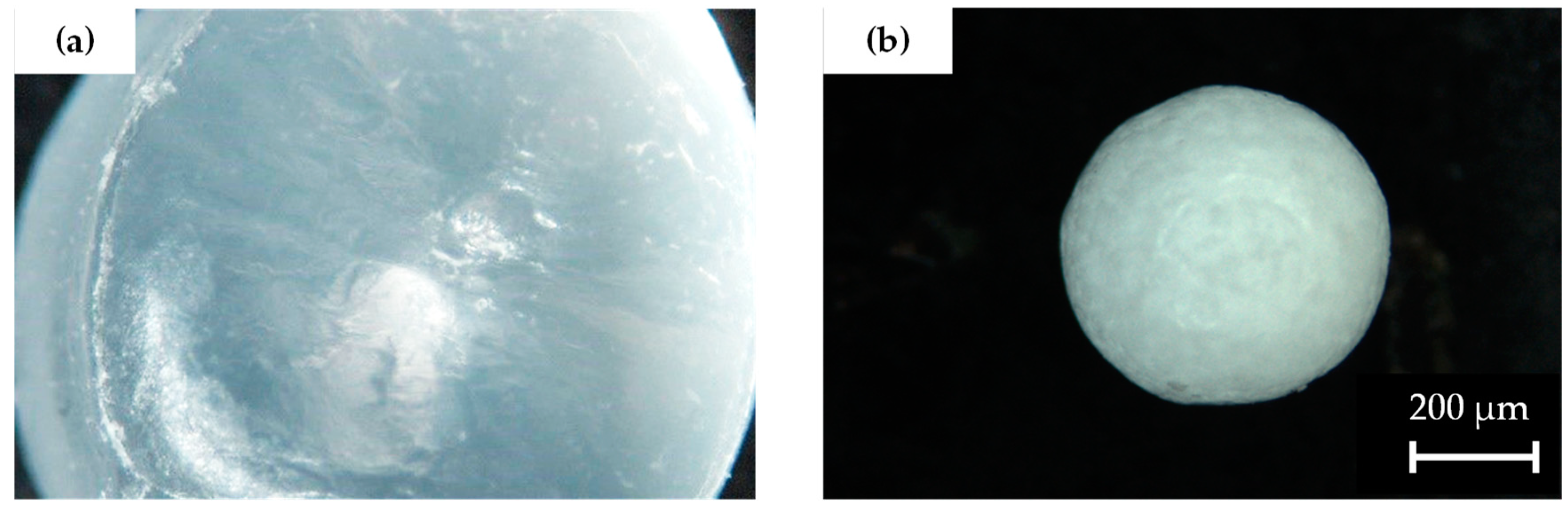
3.1. Materials
3.2. UMIM Equipment
3.3. Mechanical Properties
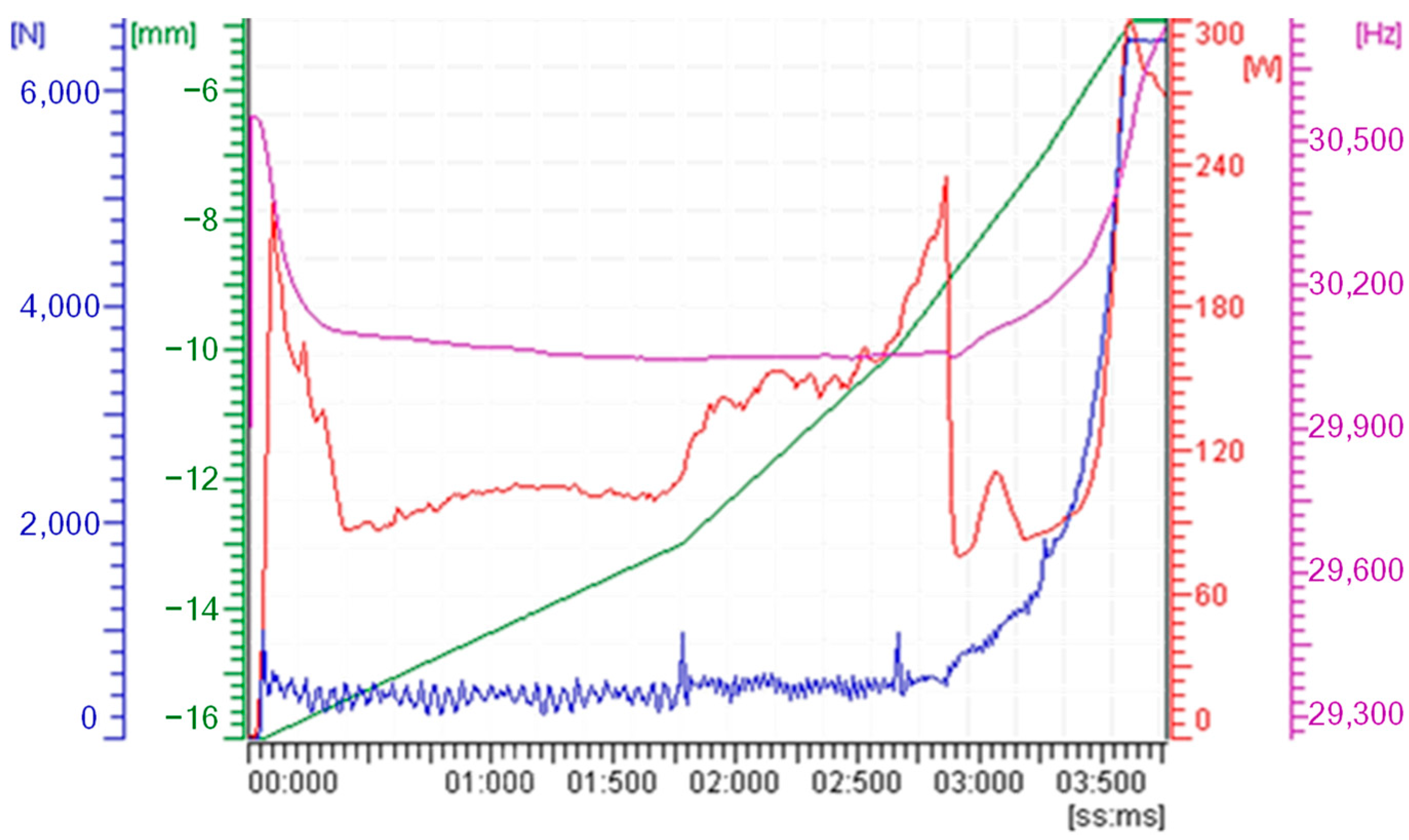
3.4. Methodology
4. Results
4.1. Energy Consumption and Mechanical Properties
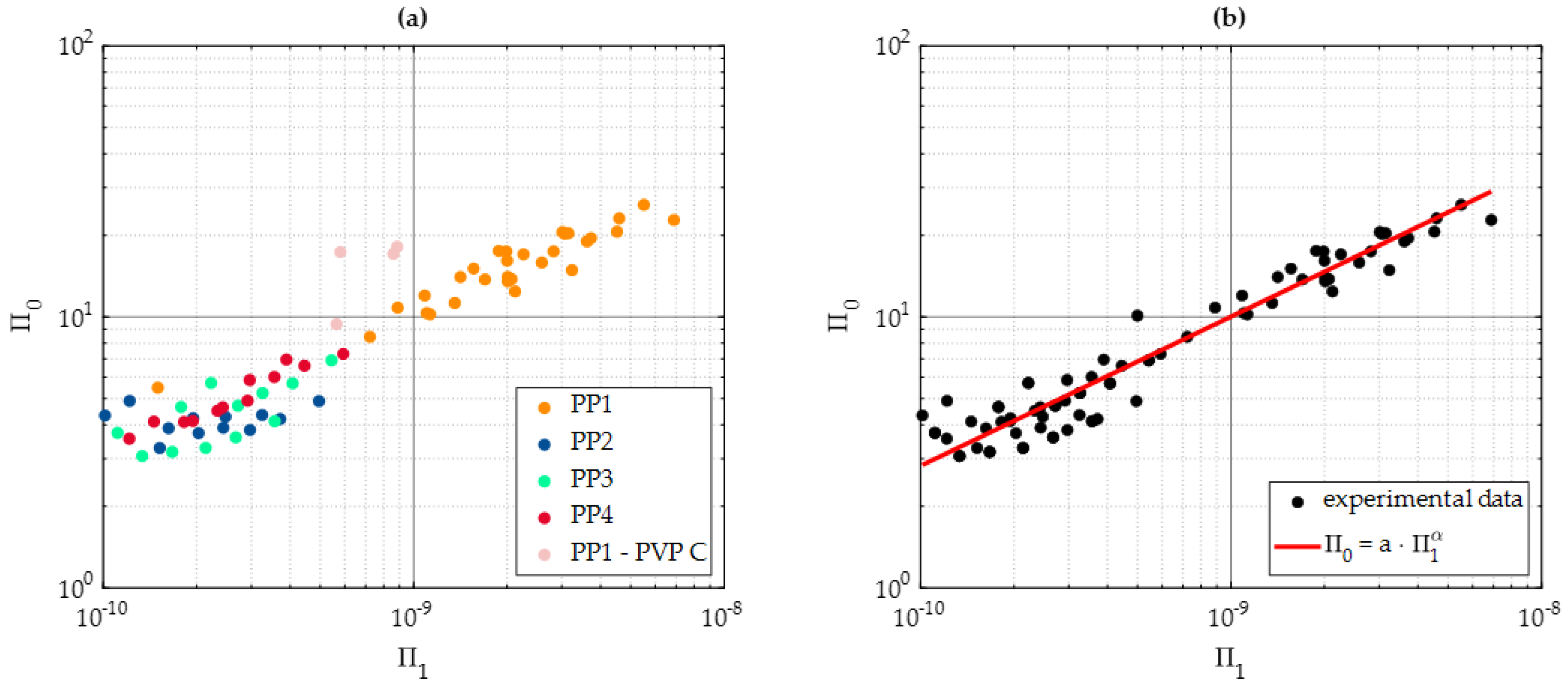
4.2. Validation of Functional Relationships for Energy Consumption
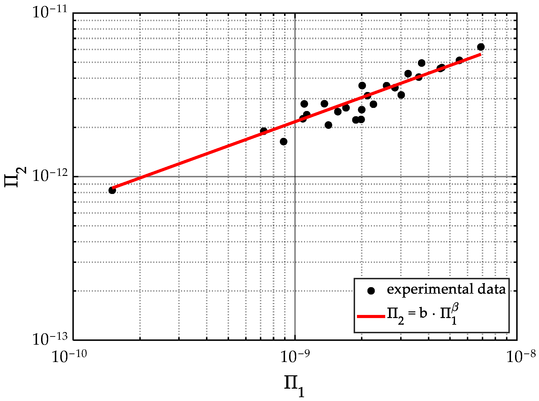
4.3. Validation of Functional Relationships for Young’s Modulus
5. Conclusions
Author Contributions
Funding
Institutional Review Board Statement
Informed Consent Statement
Data Availability Statement
Acknowledgments
Conflicts of Interest
References
- Peng, T.; Jiang, B.; Zou, Y. Study on the mechanism of interfacial friction heating in polymer ultrasonic plasticization injection molding process. Polymers 2019, 11, 1407. [Google Scholar] [CrossRef] [PubMed]
- Michaeli, W.; Kamps, T.; Hopmann, C. Manufacturing of polymer micro parts by ultrasonic plasticization and direct injection. Microsyst. Technol. 2011, 17, 243–249. [Google Scholar] [CrossRef]
- Suslick, K.S. The Chemical Effects of Ultrasound. Sci. Am. 2010, 260, 80–86. [Google Scholar] [CrossRef]
- Jiang, B.; Peng, H.; Wu, W.; Jia, Y.; Zhang, Y. Numerical simulation and experimental investigation of the viscoelastic heating mechanism in ultrasonic plasticizing of amorphous polymers for micro injection molding. Polymers 2016, 8, 199. [Google Scholar] [CrossRef]
- Elías-Grajeda, A.; Vázquez-Lepe, E.; Siller, H.R.; Perales-Martínez, I.A.; Reséndiz-Hernández, E.; Ramírez-Herrera, C.A.; Olvera-Trejo, D.; Martínez-Romero, O. Polypropylene-Based Polymer Locking Ligation System Manufacturing by the Ultrasonic Micromolding Process. Polymers 2023, 15, 3049. [Google Scholar] [CrossRef] [PubMed]
- Jiang, B.; Zou, Y.; Wei, G.; Wu, W. Evolution of interfacial friction angle and contact area of polymer pellets during the initial stage of ultrasonic plasticization. Polymers 2019, 11, 2103. [Google Scholar] [CrossRef]
- Jiang, B.; Hu, J.; Li, J. Ultrasonic plastification speed of polymer and its influencing factors. J. Cent. South Univ. 2012, 19, 380–383. [Google Scholar] [CrossRef]
- Dorf, T.; Ferrer, I.; Ciurana, J. The effect of weld line on tensile strength of polyphenylsulfone (PPSU) in ultrasonic micro-moulding technology. Int. J. Adv. Manuf. Technol. 2019, 103, 2391–2400. [Google Scholar] [CrossRef]
- Wu, W.; Pan, L.; Li, B.; He, X.; Jiang, B. Plastic rod as a promising feed material for enhanced performance of ultrasonic plasticization microinjection molding: Plasticization rate, mechanical and thermal properties. Polym. Test. 2023, 118, 1–9. [Google Scholar] [CrossRef]
- Gaxiola-Cockburn, R.; Martínez-Romero, O.; Elías-Zúñiga, A.; Olvera-Trejo, D.; Reséndiz-Hernández, J.E.; Soria-Hernández, C.G. Investigation of the Mechanical Properties of Parts Fabricated with Ultrasonic Micro Injection Molding Process Using Polypropylene Recycled Material. Polymers 2020, 12, 2033. [Google Scholar] [CrossRef]
- Gulcur, M.; Whiteside, B.R.; Nair, K.; Babenko, M.; Coates, P.D. Ultrasonic injection moulding of polypropylene and thermal visualisation of the process using a bespoke injection mould tool. In Proceedings of the Euspen’s 18th International Conference & Exhibition, Venice, Italy, 4–8 June 2018; pp. 243–244. [Google Scholar]
- Masato, D.; Babenko, M.; Shriky, B.; Gough, T.; Lucchetta, G.; Whiteside, B. Comparison of crystallization characteristics and mechanical properties of polypropylene processed by ultrasound and conventional micro-injection molding. Adv. Manuf. Technol. 2018, 99, 113–125. [Google Scholar] [CrossRef]
- Jiang, B.; Zou, Y.; Liu, T.; Wu, W. Characterization of the Fluidity of the Ultrasonic Plasticized Polymer Melt by Spiral Flow Testing under Micro-Scale. Polymers 2019, 11, 357. [Google Scholar] [CrossRef] [PubMed]
- Heredia, U.; Vázquez, E.; Ferrer, I.; Rodríguez, C.A.; Ciurana, J. Feasibility of manufacturing low aspect ratio parts of PLA by ultrasonic moulding technology. Procedia Manuf. 2017, 13, 251–258. [Google Scholar] [CrossRef]
- Michaeli, W.H.S.; Maesing, R.; Kamps, T. Injection moulding—Machine technology. In Proceedings of the 24th international IKV Plastics Technology Colloquium, Aachen, Germany, 20–21 February 2008. [Google Scholar]
- Sánchez-Sánchez, X.; Hernández-Avila, M.; Elizalde, L.E.; Martínez, O.; Ferrer, I.; Elías-Zuñiga, A. Micro injection molding processing of UHMWPE using ultrasonic vibration energy. Mater. Des. 2017, 132, 1–12. [Google Scholar] [CrossRef]
- Dorf, T.; Perkowska, K.; Janiszewska, M.; Ferrer, I.; Ciurana, J. Effect of the main process parameters on the mechanical strength of polyphenylsulfone (PPSU) in ultrasonic micro-moulding process. Ultrason. Sonochem. 2018, 46, 46–58. [Google Scholar] [CrossRef]
- Dorf, T.; Ferrer, I.; Ciurana, J. Characterizing ultrasonic micro-molding process of polyetheretherketone (PEEK). Polym. Process. 2018, 33, 442–452. [Google Scholar] [CrossRef]
- Ding, Q.; Du, M.; Liao, T.; Men, Y.; Androsch, R. Polymorphic structure in ultrasonic microinjection-molded poly (butylene-2,6-naphthalate). Polymer 2022, 257, 125275. [Google Scholar] [CrossRef]
- Sánchez-Sánchez, X.; Elias-Zuñiga, A.; Hernández-Avila, M. Processing of ultra-high molecular weight polyethylene/graphite composites by ultrasonic injection mouldingmolding: Taguchi optimization. Ultrason. Sonochem. 2018, 44, 350–358. [Google Scholar] [CrossRef]
- Olmo, C.; Amestoy, H.; Casas, M.T.; Martínez, J.C.; Franco, L.; Sarasua, J.-R.; Puiggalí, J. Preparation of nanocomposites of poly(ε-caprolactone) and multi-walled carbon nanotubes by ultrasound micro-molding. Influence of nanotubes on melting and crystallization. Polymers 2017, 9, 322. [Google Scholar] [CrossRef]
- Planellas, M.; Sacristán, M.; Rey, L.; Olmo, C.; Aymamí, J.; Casas, M.; del Valle, L.; Franco, L.; Puiggalí, J. Micro-molding with ultrasonic vibration energy: New method to disperse nanoclays in polymer matrices. Ultrason. Sonochem. 2014, 21, 1557–1569. [Google Scholar] [CrossRef]
- Díaz, A.; Franco, L.; Casas, M.T.; del Valle, L.J.; Aymamí, J.; Olmo, C. Preparation of micro-molded exfoliated clay nanocomposites by means of ultrasonic technology. Polym. Res. 2014, 21, 584. [Google Scholar] [CrossRef]
- Olmo, C.; Franco, L.; del Valle, L.J.; Puiggalí, J. Preparation of Medicated Polylactide Micropieces by Means of Ultrasonic Technology. Appl. Sci. 2019, 9, 2360. [Google Scholar] [CrossRef]
- Benatar, A. Ultrasonic Welding of Advanced Thermoplastic Composites. Ph.D. Thesis, Massachusetts Institute of Technology, Cambridge, MA, USA, 1987. [Google Scholar]
- Wu, W.; Peng, H.; Jia, Y.; Jiang, B. Characteristics and mechanisms of polymer interfacial friction heating in ultrasonic plasticization for micro injection molding. Microsyst. Technol. 2017, 23, 1385–1392. [Google Scholar] [CrossRef]
- Wu, W.; He, C.; Qiang, Y.; Peng, H.; Zhou, M. Polymer-Metal Interfacial Friction Characteristics under Ultrasonic Plasticizing Conditions: A United-Atom Molecular Dynamic Study. Mol. Sci. 2022, 23, 2829. [Google Scholar] [CrossRef] [PubMed]
- Marhöfer, D.M.; Tosello, G.; Hansen, H.N.; Islam, A. Advancements on the simulation of the micro injection molding process. In Proceedings of the 10th International Conference on Multi-Material Micro Manufacture, San Sebastián, Spain, 8–10 October 2013; pp. 77–81. [Google Scholar]
- Grabalosa, J.; Ferrer, I.; Elías-Zúñiga, A.; Ciurana, J. Influence of processing conditions on manufacturing polyamide parts by ultrasonic molding. Mater. Des. 2016, 98, 20–30. [Google Scholar] [CrossRef]
- Janer, M.; Plantà, X.; Riera, D. Ultrasonic moulding: Current state of the technology. Ultrasonics 2020, 102, 106038. [Google Scholar] [CrossRef] [PubMed]
- Gülcür, M.; Brown, E.; Gough, T.; Romano, J.-M.; Penchev, P.; Dimov, S.; Whiteside, B. Ultrasonic micromoulding: Process characterization using extensive in-line monitoring for micro-scaled products. J. Manuf. Process. 2020, 58, 289–301. [Google Scholar] [CrossRef]
- Clerk-Maxwell, J. Remarks on the Mathematical Classification of Physical Quantities. Proc. Lond. Math. Soc. 1869, s1–s3, 224–233. [Google Scholar] [CrossRef]
- Tan, Q.-M. Dimensional Analysis: With Case Studies in Mechanics; Springer: Berlin/Heidelberg, Germany, 2011. [Google Scholar]
- Sonin, A.A. The Physical Basis of Dimensional Analysis; MIT: Cambridge, UK, 2001. [Google Scholar]
- Abdelbary, A. Prediction of wear in polymers and their composites. In Wear of Polymers and Composites; Woodhead Publishing: Sawston, UK, 2014. [Google Scholar]
- Diabb, J.; Rodríguez, C.A.; Mamidi, N.; Sandoval, J.A.; Taha-Tijerina, J.; Martínez-Romero, O.; Elías-Zúñiga, A. Study of lubrication and wear in single point incremental sheet forming (SPIF) process using vegetable oil nanolubricants. Wear 2017, 376–377, 777–785. [Google Scholar] [CrossRef]
- Sakashita, H.; Tsuruta, T.; Nagai, N.; Mori, S.; Shoji, M.; Haramura, Y.; Ohtake, H.; Liu, W.; Umekawa, H.; Koizumi, Y.; et al. CHF-Transition Boiling; Elsevier: Amsterdam, The Netherlands, 2017. [Google Scholar]
- Gullberg, P.; Sengupta, R.; Horrigan, K. Transient Fan Modelling and Effects of Blade Deformation in a Truck Cooling Fan Installation; Woodhead Publishing Limited: Sawston, UK, 2013. [Google Scholar]
- Estrada-Díaz, J.A.; Elías-Zúñiga, A.; Martínez-Romero, O.; Rodríguez-Salinas, J.; Olvera-Trejo, D. A mathematical dimensionless model for electrohydrodynamics. Results Phys. 2021, 25, 104256. [Google Scholar] [CrossRef]
- Dhutekar, P.; Mehta, G.; Modak, J.; Shelare, S.; Belkhode, P. Establishment of mathematical model for minimization of human energy in a plastic moulding operation. Mater. Today Proc. 2021, 47, 4502–4507. [Google Scholar] [CrossRef]
- Gibbings, J.C. Dimensional Analysis; Springer: London, UK, 2011. [Google Scholar]
- Ferrer, I.; Vives-Mestres, M.; Manresa, A.; Garcia-Romeu, M.L. Replicability of ultrasonic molding for processing thin-wall polystyrene plates with a microchannel. Materials 2018, 11, 1320. [Google Scholar] [CrossRef]
- Levy, A.; le Corre, S.; Poitou, A.; Soccard, E. Ultrasonic welding of thermoplastic composites: Modeling of the process using time homogenization. Multiscale Comput. Eng. 2011, 9, 53–71. [Google Scholar] [CrossRef]
- Zhang, Z.; Wang, X.; Luo, Y.; Zhang, Z.; Wang, L. Study on heating process of ultrasonic welding for thermoplastics. Thermoplast. Compos. Mater. 2010, 23, 647–664. [Google Scholar] [CrossRef]
- Grewell, A.; Benatar, D. Welding of plastics: Fundamentals and new developments. Polym. Process. 2007, 22, 43–60. [Google Scholar] [CrossRef]
- Giles, H.F., Jr.; Wagner, J.R., Jr.; Mount, E.M., III. Extrusion: The Definitive Processing Guide and Handbook; William Andrew: Norwich, NY, USA, 2014; pp. 195–204. [Google Scholar]
- Balani, K.; Verma, V.; Agarwal, A.; Narayan, R. Physical, Thermal, and Mechanical Properties of Polymers. In Biosurfaces; John Wiley & Sons, Inc.: Hoboken, NJ, USA, 2015; pp. 329–344. [Google Scholar]
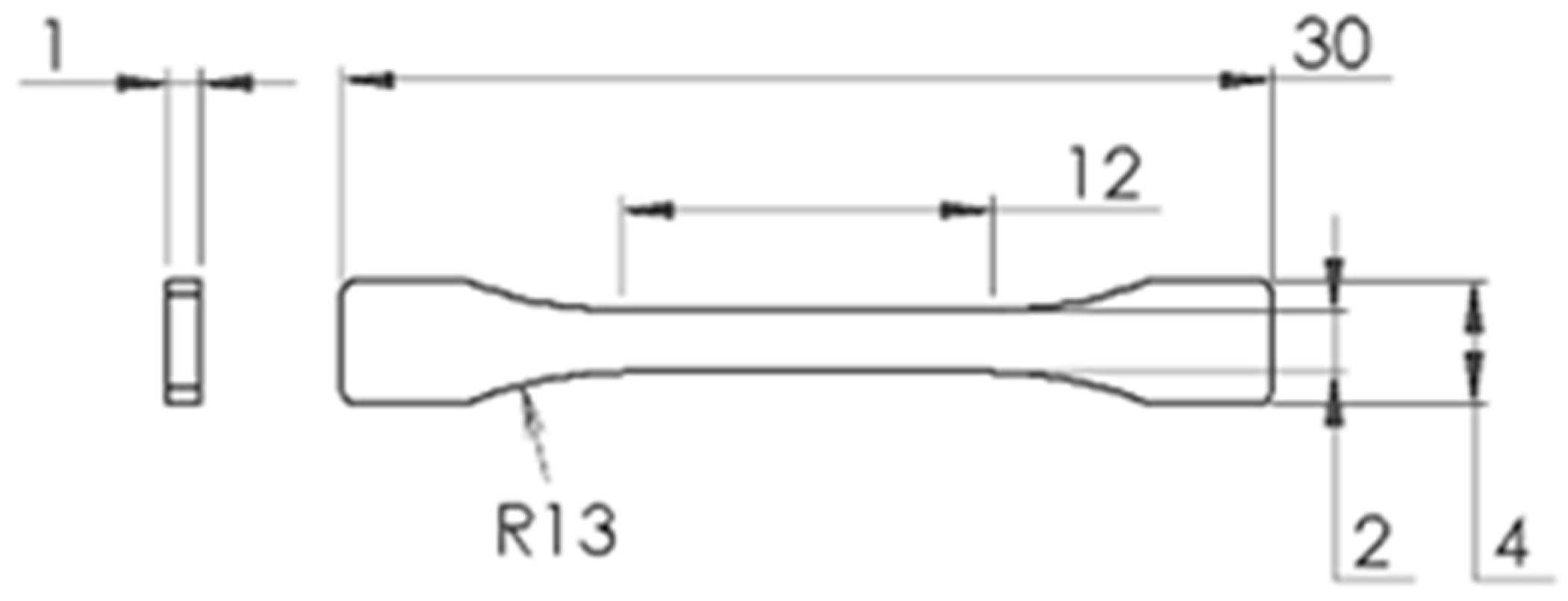
- ASTM D638-14; Standard Test Method for Tensile Properties of Plastics. ASTM International: West Conshohocken, PA, USA, 2014.
- Olefins, I. Typical Engineering Properties of Polypropylene; INEOS Olefins & Polymers USA: Texas, TX, USA, 2010; p. 2. [Google Scholar]
- Estrada-Díaz, J.A.; Elías-Zúñiga, A.; Martínez-Romero, O.; Rodríguez-Salinas, J.; Olvera-Trejo, D. Mathematical Dimensional Model for Predicting Bulk Density of Inconel 718 Parts Produced by Selective Laser Melting. Materials 2021, 14, 512. [Google Scholar] [CrossRef]
- Estrada-Díaz, J.A.; Elías-Zúñiga, A.; Martínez-Romero, O.; Rodríguez-Salinas, J.; Olvera-Trejo, D. Enhanced Mathematical Model for Producing Highly Dense Metallic Components through Selective Laser Melting. Materials 2021, 14, 1571. [Google Scholar] [CrossRef]


| Variable (Parameter Process) | Variable (Material Properties) | Variable Symbol | Dimensions | SI Units |
|---|---|---|---|---|
| Amplitude | A | m | ||
| Energy consumption | Q | J | ||
| Flexural modulus | SF | Pa | ||
| Injection force | IF | N | ||
| Injection speed | IS | m/s | ||
| Mold temperature | TM | °K | ||
| Plunger power | P | W | ||
| Thermal conductivity coefficient | λ | W/(m·°K) | ||
| Ultrasonic time | Ut | S | ||
| Young’s modulus | E | Pa |
| Properties | Polypropylene Homopolymer Axlene12 (PP1) | Polypropylene Homopolymer HG619N (PP2) | Polypropylene Homopolymer HS013 (PP3) | Polypropylene Homopolymer HG613NW (PP4) |
|---|---|---|---|---|
| Melt flow index (g/10 min) | 12 | 35 | 11 | 20 |
| Yield strength (MPa) | 33 | 33 | 34 | 36 |
| Yield strain (%) | 10 | 8 | 10 | 9 |
| Notched Izod impact at 23 °C (J/m) | 33 | 15.4 | 26 | 26 |
| Flexural modulus (MPa) | 1400 | 1700 | 1420 | 1558 |
| Density (g/cm3) | 0.9 | 0.9 | 0.9 | 0.9 |
| Heat deflection temperature at 0.46 MPa (°C) | 104 | 115 | 94 | 111 |
| Technical Specifications | |||
|---|---|---|---|
| Ultrasonic frequency | 30 kHz | Clamping force | 30 kN |
| Max. ultrasonic amplitude | 56.2 μm | Molding pressure | 300 bars (approx.) |
| Power level | 1.5 kW | Max. shot volume | 1 cm3 |
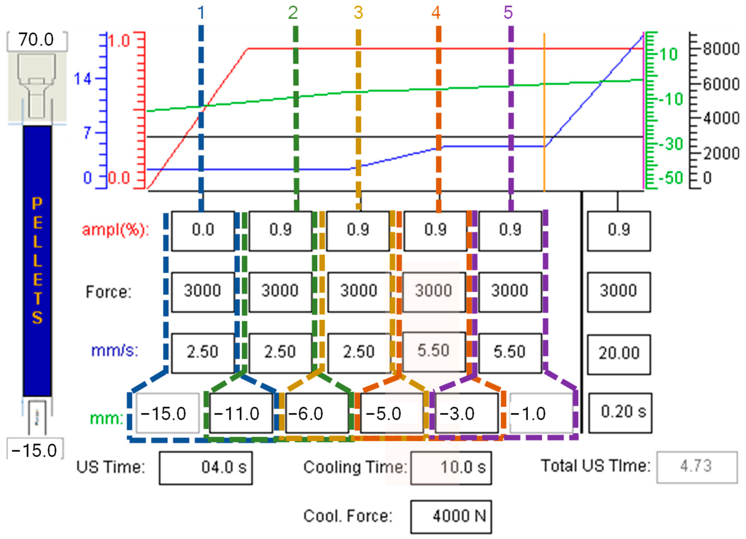
| Plunger Velocity Profile | Stage 1 | Stage 2 | Stage 3 | Stage 4 | Stage 5 | Injection Speed (IS) (mm/s) |
|---|---|---|---|---|---|---|
| PVP A | 1.8 | 3.4 | 5.0 | 6.0 | 9.0 | 3.72 |
| PVP B | 2.5 | 2.5 | 2.5 | 5.5 | 5.5 | 2.92 |
| PVP C | 5.5 | 5.5 | 5.5 | 5.5 | 5.5 | 5.50 |
| PVP D | 2.5 | 3.5 | 4.5 | 5.5 | 6.5 | 3.60 |
| PVP E | 2.0 | 3.0 | 3.5 | 5.0 | 5.5 | 2.98 |
| PVP F | 3.0 | 3.5 | 4.0 | 4.5 | 5.0 | 3.65 |
| PVP G | 3.5 | 3.5 | 3.5 | 6.5 | 6.5 | 4.03 |
| Processing Parameter | Exp. 1 | Exp. 2 | Exp. 3 | Exp. 4 | Exp. 5 | Exp. 6 | Exp. 7 | Exp. 8 |
|---|---|---|---|---|---|---|---|---|
| A (%) | 90 | 100 | 80 | 90 | 100 | 80 | 90 | 100 |
| Ut (s) | 4 | 4 | (3, 4, 5, 6) | (3, 4, 5, 6) | (3, 4, 5, 6) | (4, 5, 6) | (4, 5, 6) | (4, 5, 6) |
| TM (°C) | (80, 90) | (80, 90) | 50 | 50 | 50 | (80, 100) | (80, 100) | (80, 100) |
| PVP | (B, C) | (B, C) | A | A | A | B, D, E, F, G | B, D, E, F, G | B, D, E, F, G |
| IF (kN) | 3.0 | 3.0 | 6.5 | 6.5 | 6.5 | (2, 3, 4, 5) | (2, 3, 4, 5) | (2, 3, 4, 5) |
| Material | PP1 | PP1 | PP2, PP3, PP4 | PP2, PP3, PP4 | PP2, PP3, PP4 | PP1 | PP1 | PP1 |
| A (%) | PVP | TM (°C) | Qavg PP1 (J) | CI (J) |
|---|---|---|---|---|
| 90 | B | 80 | 473.93 | (449.8, 498.1) |
| 90 | 483.13 | (458.0, 508.3) | ||
| C | 80 | 621.00 | (549.5, 692.5) | |
| 90 | 1146.47 | (995.5, 1297.4) | ||
| 100 | B | 80 | 709.73 | (659.6, 759.8) |
| 90 | 712.87 | (668.9, 756.8) | ||
| C | 80 | 1129.43 | (942.8, 1316.1) | |
| 90 | 1198.20 | (1054.0, 1342.4) |
| A (%) | Ut (s) | Qavg PP2 (J) | CI (J) | Qavg PP3 (J) | CI (J) | Qavg PP4 (J) | CI (J) |
|---|---|---|---|---|---|---|---|
| 80 | 3 | 336.92 | (320.6, 353.3) | 270.75 | (260.2, 281.3) | 415.5 | (407.2, 423.8) |
| 4 | 396.83 | (388.0, 405.7) | 318.17 | (304.7, 331.6) | 307.58 | (293.2, 322.0) | |
| 5 | 497.67 | (480.5, 514.8) | 593.25 | (577.4, 609.1) | 371.25 | (356.7, 385.8) | |
| 6 | 516.42 | (509.7, 523.1) | 629.25 | (609.3, 649.2) | 542.58 | (529.2, 555.9) | |
| 90 | 3 | 505.5 | (495.0, 516.0) | 315.75 | (304.7, 326.8) | 299.5 | (286.3, 312.7) |
| 4 | 475.58 | (468.7, 482.5) | 377.75 | (366.5, 389.0) | 348.08 | (337.9, 358.3) | |
| 5 | 545.42 | (537.7, 553.1) | 512.42 | (502.2, 522.6) | 398 | (387.2, 408.8) | |
| 6 | 600.33 | (581.4, 619.3) | 564.18 | (542.2, 586.1) | 675.92 | (652.1, 699.8) | |
| 100 | 3 | 530.33 | (513.4, 547.3) | 355.17 | (346.8, 363.5) | 502.25 | (469.4, 535.1) |
| 4 | 639.58 | (628.5, 650.7) | 407 | (395.0, 419.0) | 550.92 | (543.4, 558.4) | |
| 5 | 727 | (706.1, 747.9) | 463.42 | (407.1, 519.8) | 634.25 | (626.9, 641.6) | |
| 6 | 849.71 | (843.0, 856.5) | 622 | (564.6, 679.4) | 683.42 | (643.5, 723.4) |
| A (%) | TM (°C) | Ut (s) | IF (N) | IS (mm/s) | PVP | Qavg (J) | CI (J) | Avg. Maximum Stress (MPa) | Avg. Young’s Modulus (MPa) | ID |
|---|---|---|---|---|---|---|---|---|---|---|
| 80 | 50 | 4 | 6500 | 3.7221 | A | 531.00 | (479.0, 583.0) | 23.52 | 878.47 | 1 |
| 80 | 4 | 2000 | 2.9167 | B | 407.60 | (381.8, 433.4) | 27.80 | 898.20 | 2 | |
| 5 | 497.00 | (457.0, 537.0) | 28.65 | 888.94 | 3 | |||||
| 6 | 613.60 | (488.6, 738.6) | 26.68 | 855.62 | 4 | |||||
| 100 | 4 | 4.0316 | G | 486.80 | (449.5, 524.1) | 23.87 | 799.52 | 5 | ||
| 6 | 2.9167 | B | 611.40 | (562.2, 660.6) | 28.02 | 885.46 | 6 | |||
| 90 | 80 | 4 | 2000 | 2.9167 | B | 481.60 | (432.1, 531.1) | 29.63 | 826.46 | 7 |
| 3000 | 492.00 | (452.5. 531.5) | 43.26 | 974.47 | 8 | |||||
| 4000 | 477.60 | (448.0, 507.2) | 30.53 | 862.62 | 9 | |||||
| 5000 | 493.00 | (456.3, 529.7) | 27.51 | 854.85 | 10 | |||||
| 5 | 2000 | 554.80 | (500.1, 609.5) | 28.02 | 915.17 | 11 | ||||
| 6 | 719.80 | (680.5, 759.1) | 28.85 | 854.19 | 12 | |||||
| 100 | 4 | 2000 | 4.0316 | G | 651.00 | (603.9, 698.1) | 23.59 | 821.63 | 13 | |
| 5 | 3000 | 654.75 | (614.7, 694.8) | 24.94 | 765.29 | 14 | ||||
| 4 | 3000 | 2.9167 | B | 434.80 | (423.6, 446.0) | 30.51 | 891.03 | 15 | ||
| 3.6473 | F | 493.00 | (470.2, 515.8) | 25.52 | 954.51 | 16 | ||||
| 5 | 2.9167 | B | 601.60 | (596.4, 606.8) | 26.10 | 838.63 | 17 | |||
| 3.6473 | F | 656.40 | (583.3, 729.5) | 26.92 | 844.94 | 18 | ||||
| 6 | 2.9167 | B | 737.20 | (676.6, 797.8) | 23.17 | 840.22 | 19 | |||
| 100 | 80 | 4 | 2000 | 2.9167 | B | 531.80 | (488.7, 574.9) | 24.27 | 815.34 | 20 |
| 5 | 756.40 | (666.9, 845.9) | 24.91 | 844.19 | 21 | |||||
| 6 | 809.00 | (457.0, 537.0) | 27.72 | 915.15 | 22 | |||||
| 4 | 4000 | 3.6473 | F | 603.60 | (558.1, 649.1) | 17.42 | 1016.89 | 23 | ||
| 100 | 5 | 2000 | 712.80 | (616.9, 808.7) | 26.01 | 943.96 | 24 | |||
| 4 | 3000 | 2.9167 | B | 521.20 | (492.2, 550.2) | 28.02 | 886.63 | 25 | ||
| 5 | 694.80 | (622.6, 767.0) | 23.64 | 861.35 | 26 |
| Coefficient | Value | Confidence Interval, CI (J) |
|---|---|---|
| a | 9.046 × 10⁵ | (3.844 × 10⁵, 1.425 × 10⁶) |
| 0.5506 | (0.5217, 0.5794) |
| Coefficient | Value | Confidence Interval, CI (J) |
|---|---|---|
| b | 5.821 × 10⁻⁸ | (−5.322 × 10⁻⁸, 1.696 × 10⁻⁷) |
| 0.4921 | (0.3947, 0.5896) |
Disclaimer/Publisher’s Note: The statements, opinions and data contained in all publications are solely those of the individual author(s) and contributor(s) and not of MDPI and/or the editor(s). MDPI and/or the editor(s) disclaim responsibility for any injury to people or property resulting from any ideas, methods, instructions or products referred to in the content. |
© 2023 by the authors. Licensee MDPI, Basel, Switzerland. This article is an open access article distributed under the terms and conditions of the Creative Commons Attribution (CC BY) license (https://creativecommons.org/licenses/by/4.0/).
Share and Cite
Salazar-Meza, M.; Martínez-Romero, O.; Reséndiz-Hernández, J.E.; Olvera-Trejo, D.; Estrada-Díaz, J.A.; Ramírez-Herrera, C.A.; Elías-Zúñiga, A. Modeling the Ultrasonic Micro-Injection Molding Process Using the Buckingham Pi Theorem. Polymers 2023, 15, 3779. https://doi.org/10.3390/polym15183779
Salazar-Meza M, Martínez-Romero O, Reséndiz-Hernández JE, Olvera-Trejo D, Estrada-Díaz JA, Ramírez-Herrera CA, Elías-Zúñiga A. Modeling the Ultrasonic Micro-Injection Molding Process Using the Buckingham Pi Theorem. Polymers. 2023; 15(18):3779. https://doi.org/10.3390/polym15183779
Chicago/Turabian StyleSalazar-Meza, Marco, Oscar Martínez-Romero, José Emiliano Reséndiz-Hernández, Daniel Olvera-Trejo, Jorge Alfredo Estrada-Díaz, Claudia Angélica Ramírez-Herrera, and Alex Elías-Zúñiga. 2023. "Modeling the Ultrasonic Micro-Injection Molding Process Using the Buckingham Pi Theorem" Polymers 15, no. 18: 3779. https://doi.org/10.3390/polym15183779
APA StyleSalazar-Meza, M., Martínez-Romero, O., Reséndiz-Hernández, J. E., Olvera-Trejo, D., Estrada-Díaz, J. A., Ramírez-Herrera, C. A., & Elías-Zúñiga, A. (2023). Modeling the Ultrasonic Micro-Injection Molding Process Using the Buckingham Pi Theorem. Polymers, 15(18), 3779. https://doi.org/10.3390/polym15183779