
A Novel Approach for Simulation and Optimization of Rubber Vulcanization

Abstract
:1. Introduction
2. Materials and Methods
2.1. Materials
2.2. Simulation
- Minimal vulcanization degree ();
- Average vulcanization degree ();
- Maximal vulcanization degree ();
- Minimal temperature ();
- Average temperature ();
- Maximal temperature ();
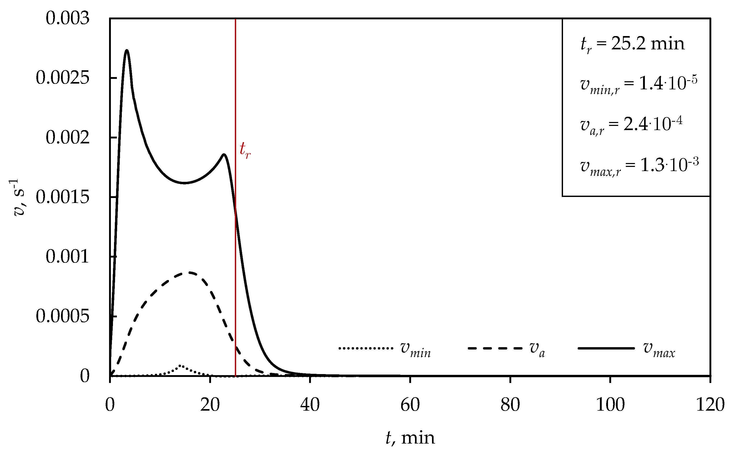
- Minimal vulcanization rate ();
- Average vulcanization rate ();
- Maximal vulcanization rate ().
3. Results and Discussion
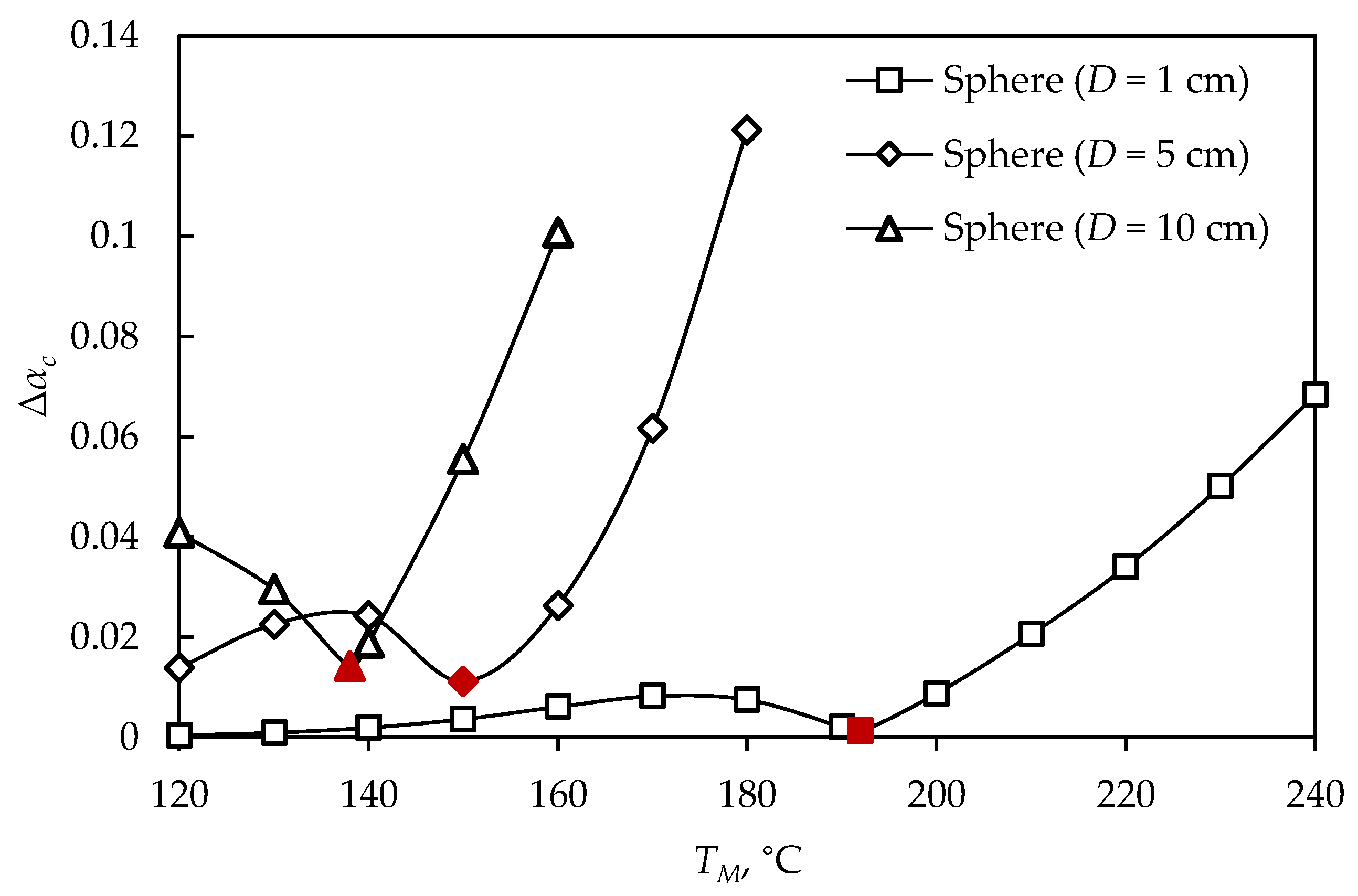
3.1. Simulation of Vulcanization of a Sphere of Different Dimensions
3.2. Simulation of Vulcanization of Rubber Wheels
4. Conclusions
Author Contributions
Funding
Institutional Review Board Statement
Informed Consent Statement
Data Availability Statement
Acknowledgments
Conflicts of Interest
List of Variables and Their Definitions
References
- Tavakoli, M.; Katbab, A.A.; Nazockdast, H. NR/SBR/organoclay nanocomposites: Effects of molecular interactions upon the clay microstructure and mechano-dynamic properties. J. Appl. Polym. Sci. 2012, 123, 1853–1864. [Google Scholar]
- Shen, J.; Wen, S.; Du, Y.; Li, N.; Zhang, L.; Yang, Y.; Liu, L. The network and properties of the NR/SBR vulcanizate modified by electron beam irradiation. Radiat. Phys. Chem. 2013, 92, 99–104. [Google Scholar]
- Xiang, H.; Yin, J.; Lin, G.; Liu, X.; Rong, M.; Zhang, M. Photo-crosslinkable, self-healable and reprocessable rubbers. Chem. Eng. J. 2019, 358, 879–890. [Google Scholar]
- Ortega, L.; Cerveny, S.; Sill, C.; Isitman, N.A.; Rodriguez-Garraza, A.L.; Meyer, M.; Westermann, S.; Schwartz, G.A. The effect of vulcanization additives on the dielectric response of styrene-butadiene rubber compounds. Polymer 2019, 172, 205–212. [Google Scholar] [CrossRef]
- Ghoreishy, M.H.R. A state-of-the-art review on the mathematical modelling and computer simulation of rubber vulcanization process. Iran. Polym. J. 2016, 25, 89–109. [Google Scholar] [CrossRef]
- Lopes, H.; Silva, S.P.; Carvalho, J.P.; Machado, J. A new modelling approach for predicting process evolution of cork-rubber composites slabs vulcanization. Sci. Rep. 2022, 12, 8002. [Google Scholar]
- Arrillaga, A.; Zaldua, A.M.; Atxurra, R.M.; Farid, A.S. Techniques used for determining cure kinetics of rubber compounds. Eur. Polym. J. 2007, 43, 4783–4799. [Google Scholar] [CrossRef]
- Milani, G.; Milani, F. A three-function numerical model for the prediction of vulcanization-reversion of rubber during sulfur curing. J. Appl. Polym. Sci. 2011, 119, 419–437. [Google Scholar] [CrossRef]
- Rabiei, S.; Shojaei, A. Vulcanization kinetics and reversion behavior of natural rubber/styrene-butadiene rubber blend filled with nanodiamond–The role of sulfur curing system. Eur. Polym. J. 2016, 81, 98–113. [Google Scholar] [CrossRef]
- Kader, M.A.; Nah, C. Influence of clay on the vulcanization kinetics of fluoroelastomer nanocomposites. Polymer 2004, 45, 2237–2247. [Google Scholar] [CrossRef]
- Khang, T.H.; Ariff, Z.M. Vulcanization kinetics study of natural rubber compounds having different formulation variables. J. Therm. Anal. Calorim. 2012, 109, 1545–1553. [Google Scholar] [CrossRef]
- Mathew, G.; Rhee, J.M.; Lee, Y.S.; Park, D.H.; Nah, C. Cure kinetics of ethylene acrylate rubber/clay nanocomposites. J. Ind. Eng. Chem. 2008, 14, 60–65. [Google Scholar] [CrossRef]
- Sui, G.; Zhong, W.H.; Yang, X.P.; Yu, Y.H.; Zhao, S.H. Preparation and properties of natural rubber composites reinforced with pretreated carbon nanotubes. Polym. Adv. Technol. 2008, 19, 1543–1549. [Google Scholar]
- Wu, J.; Xing, W.; Huang, G.; Li, H.; Tang, M.; Wu, S.; Liu, Y. Vulcanization kinetics of graphene/natural rubber nanocomposites. Polymer 2013, 54, 3314–3323. [Google Scholar] [CrossRef]
- Choi, D.; Kader, M.A.; Cho, B.H.; Huh, Y.I.; Nah, C. Vulcanization kinetics of nitrile rubber/layered clay nanocomposites. J. Appl. Polym. Sci. 2005, 98, 1688–1696. [Google Scholar] [CrossRef]
- Milani, G.; Milani, F. Parabola-Hyperbola PH kinetic model for NR sulphur vulcanization. Polym. Test. 2017, 58, 104–115. [Google Scholar] [CrossRef]
- Ding, R.; Leonov, A.I. A kinetic model for sulfur accelerated vulcanization of a natural rubber compound. J. Appl. Polym. Sci. 1996, 61, 455–463. [Google Scholar] [CrossRef]
- Han, I.S.; Chung, C.B.; Kang, S.J.; Kim, S.J.; Jung, H.C. A kinetic model of reversion type cure for rubber compound. Polymer 1998, 22, 223. [Google Scholar]
- Milani, G.; Milani, F. Direct and closed form analytical model for the prediction of reaction kinetic of EPDM accelerated sulphur vulcanization. J. Math. Chem. 2012, 50, 2577–2605. [Google Scholar] [CrossRef]
- Milani, G.; Milani, F. Simple kinetic numerical model based on rheometer data for Ethylene–Propylene–Diene Monomer accelerated sulfur crosslinking. J. Appl. Polym. Sci. 2012, 124, 311–324. [Google Scholar] [CrossRef]
- Isayev, A.I.; Sobhanie, M.; Deng, J.S. Two-dimensional simulation of injection molding of rubber compounds. Rubber Chem. Technol. 1988, 61, 906–937. [Google Scholar] [CrossRef]
- Adam, Q.; Behnke, R.; Kaliske, M. A thermo-mechanical finite element material model for the rubber forming and vulcanization process: From unvulcanized to vulcanized rubber. Int. J. Solids Struct. 2020, 185, 365–379. [Google Scholar] [CrossRef]
- Yao, W.G.; Jia, Y.X.; Wang, X.X. Kinetic modelling and finite element simulation of natural rubber non-isothermal vulcanization. Adv. Mater. Res. 2011, 306, 649–653. [Google Scholar] [CrossRef]
- Jia, Y.; Sun, S.; Xue, S.; Liu, L.; Zhao, G. Numerical simulation of moldable silicone rubber vulcanization process based on thermal coupling analysis. Polym. Plast. Technol. Eng. 2003, 42, 883–898. [Google Scholar] [CrossRef]
- Shi, F.; Dong, X. Three-dimension numerical simulation for vulcanization process based on unstructured tetrahedron mesh. J. Manuf. Process. 2016, 22, 1–6. [Google Scholar] [CrossRef]
- Guo, Z.S.; Du, S.; Zhang, B. Temperature field of thick thermoset composite laminates during cure process. Compos. Sci. Technol. 2005, 65, 517–523. [Google Scholar] [CrossRef]
- Park, H.C.; Goo, N.S.; Min, K.J.; Yoon, K.J. Three-dimensional cure simulation of composite structures by the finite element method. Compos. Struct. 2003, 62, 51–57. [Google Scholar] [CrossRef]
- Park, H.C.; Lee, S.W. Cure simulation of thick composite structures using the finite element method. J. Compos. Mater. 2001, 35, 188–201. [Google Scholar] [CrossRef]
- Ramorino, G.; Girardi, M.; Agnelli, S.; Franceschini, A.; Baldi, F.; Vigano, F.; Ricco, T. Injection molding of engineering rubber components: A comparison between experimental results and numerical simulation. Int. J. Mater. Form. 2010, 3, 551–554. [Google Scholar] [CrossRef]
- Zhang, J.; Tang, W. Rubber curing process simulation based on parabola model. J. Wuhan Univ. Technol. Mater. Sci. Ed. 2013, 28, 150–156. [Google Scholar] [CrossRef]
- Wang, D.H.; Dong, Q.; Jia, Y.X. Mathematical modelling and numerical simulation of the non-isothermal in-mold vulcanization of natural rubber. Chinese J. Polym. Sci. 2015, 3, 395–403. [Google Scholar] [CrossRef]
- El Labban, A.; Mousseau, P.; Deterre, R.; Bailleul, J.L.; Sarda, A. Temperature measurement and control within moulded rubber during vulcanization process. Measurement 2009, 42, 916–926. [Google Scholar] [CrossRef]
- Gong, L.; Yang, H.; Ke, Y.; Wang, S.; Yao, X. Combined effects of hot curing conditions and reaction heat on rubber vulcanization efficiency and vulcanizate uniformity. Compos. Struct. 2019, 209, 472–480. [Google Scholar] [CrossRef]
- Wang, X.; Jia, Y.; Feng, L.; An, L. Investigation on vulcanization degree and residual stress on fabric rubber composites. Macromol. Theory. Simul. 2009, 18, 268–276. [Google Scholar] [CrossRef]
- Da Costa, H.M.; Visconte, L.L.Y.; Nunes, R.C.R.; Furtado, C.R.G. Rice husk ash filled natural rubber. I. Overall rate constant determination for the vulcanization process from rheometric data. J. Appl. Polym. Sci. 2003, 87, 1194–1203. [Google Scholar] [CrossRef]
- Vajdi, M.; Moghanlou, F.S.; Sharifianjazi, F.; Asl, M.S.; Shokouhimehr, M. A review on the Comsol Multiphysics studies of heat transfer in advanced ceramics. J. Compos. Sci. 2020, 2, 35–43. [Google Scholar] [CrossRef]
- Wang, X.; Yue, H.; Liu, G.; Zhao, Z. The application of COMSOL multiphysics in direct current method forward modelling. Procedia Earth Plan. Sci. 2011, 3, 266–272. [Google Scholar] [CrossRef] [Green Version]
- Bera, O.; Pavličević, J.; Ikonić, B.; Lubura, J.; Govedarica, D.; Kojić, P. A new approach for kinetic modelling and optimization of rubber molding. Polym. Eng. Sci. 2021, 61, 879–890. [Google Scholar] [CrossRef]
- Sae-oui, P.; Thepsuwan, U. Prediction of cure level in thick rubber cylinder using finite element analysis. Sci. 2002, 28, 385–391. [Google Scholar]
- Bekkedahl, N.; Weeks, J.J. Heats of reaction of natural rubber with sulfur. J. Res. Natl. Bur. Stand. 1969, 73, 221. [Google Scholar] [CrossRef]
- Bellander, M.; Stenberg, B.; Persson, S. Crosslinking of polybutadiene rubber without any vulcanization agent. Polym. Eng. Sci. 1998, 38, 1254–1260. [Google Scholar] [CrossRef]
- Stieger, S.; Mitsoulis, E.; Walluch, M.; Ebner, C.; Kerschbaumer, R.C.; Haselmann, M.; Mostafaiyan, M.; Kämpfe, M.; Kühnert, I.; Wießner, S.; et al. On the influence of viscoelastic modelling in fluid flow simulations of gum acrylonitrile butadiene rubber. Polymers 2021, 13, 2323. [Google Scholar] [CrossRef] [PubMed]


| Heat Transfer | |
|---|---|
| Heat transfer equation | |
| Conductivity | |
| Convection | |
| Heat Source | |
| Limit conditions and values | |
| = 25 °C | |
| = 1.82 kJ kg K [38] | |
| = 1020 kg m [38] | |
| = 0.28 W m K [38] | |
| K = 0.15 mm s [38] | |
| = 13 kJ kg [40] | |
| Solutions | T(r, z, t) |
| , , | |
| Kinetic model | |
| Equations | |
| Limit conditions and values | |
| = −5.335 [38] | |
| = 0.019662 K [38] | |
| = −1.479744 [38] | |
| = 0.003896 K [38] | |
| = 85.008 kJ mol [38] | |
| = 1.017 × 10 [38] | |
| = 69.187 kJ mol [38] | |
| = 8.639 × 10 [38] | |
| Solutions | |
| , , | |
| , , | |
Disclaimer/Publisher’s Note: The statements, opinions and data contained in all publications are solely those of the individual author(s) and contributor(s) and not of MDPI and/or the editor(s). MDPI and/or the editor(s) disclaim responsibility for any injury to people or property resulting from any ideas, methods, instructions or products referred to in the content. |
© 2023 by the authors. Licensee MDPI, Basel, Switzerland. This article is an open access article distributed under the terms and conditions of the Creative Commons Attribution (CC BY) license (https://creativecommons.org/licenses/by/4.0/).
Share and Cite
Lubura, J.; Kojić, P.; Pavličević, J.; Ikonić, B.; Balaban, D.; Bera, O. A Novel Approach for Simulation and Optimization of Rubber Vulcanization. Polymers 2023, 15, 1750. https://doi.org/10.3390/polym15071750
Lubura J, Kojić P, Pavličević J, Ikonić B, Balaban D, Bera O. A Novel Approach for Simulation and Optimization of Rubber Vulcanization. Polymers. 2023; 15(7):1750. https://doi.org/10.3390/polym15071750
Chicago/Turabian StyleLubura, Jelena, Predrag Kojić, Jelena Pavličević, Bojana Ikonić, Dario Balaban, and Oskar Bera. 2023. "A Novel Approach for Simulation and Optimization of Rubber Vulcanization" Polymers 15, no. 7: 1750. https://doi.org/10.3390/polym15071750