
A Numerical Model to Predict the Relaxation Phenomena in Thermoset Polymers and Their Effects on Residual Stress during Curing, Part II: Numerical Evaluation of Residual Stress


Abstract
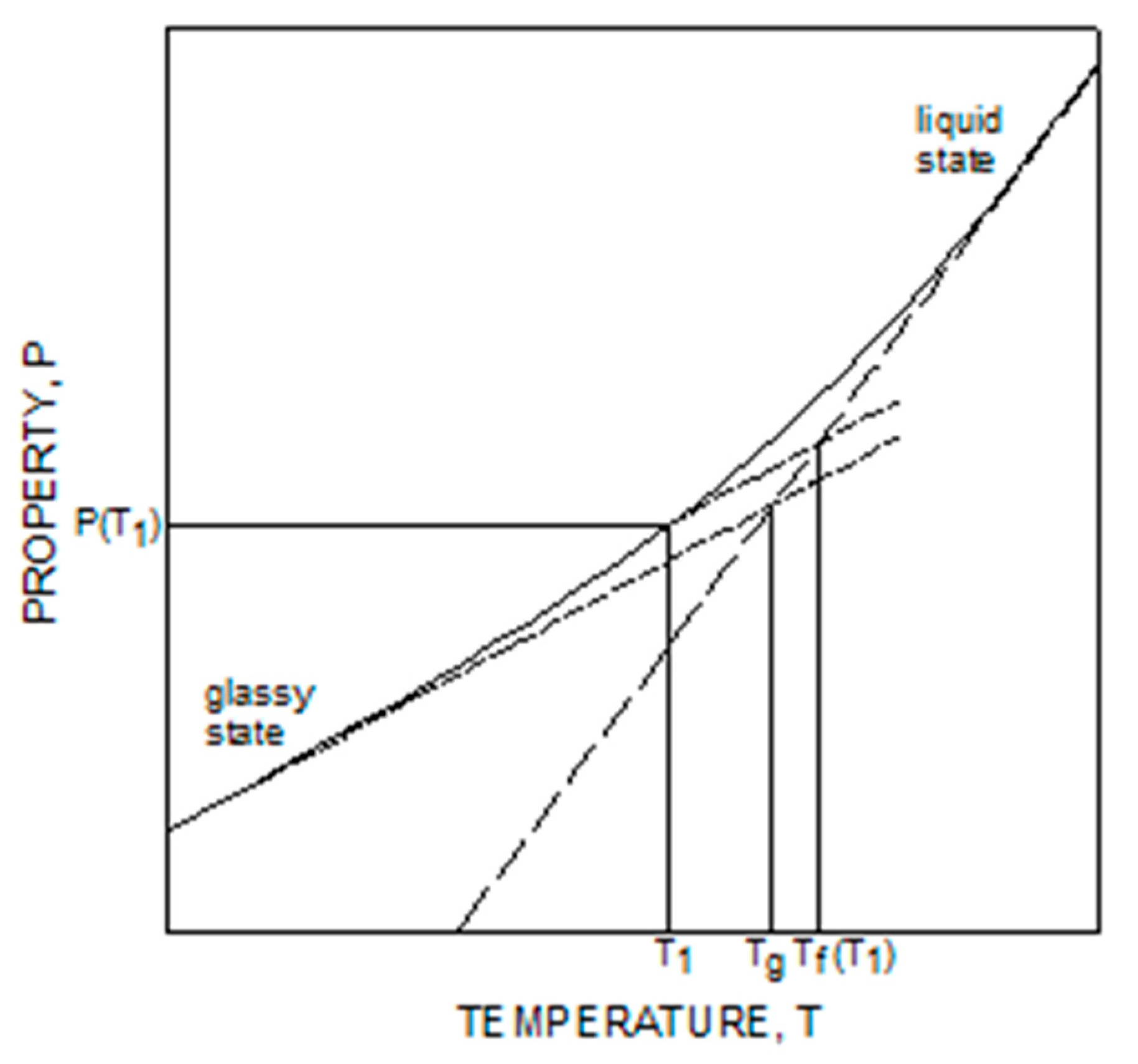
1. Introduction
2. Materials and Methods
2.1. Mathematical Formulation
2.2. FEM Model
2.3. Model Parameters
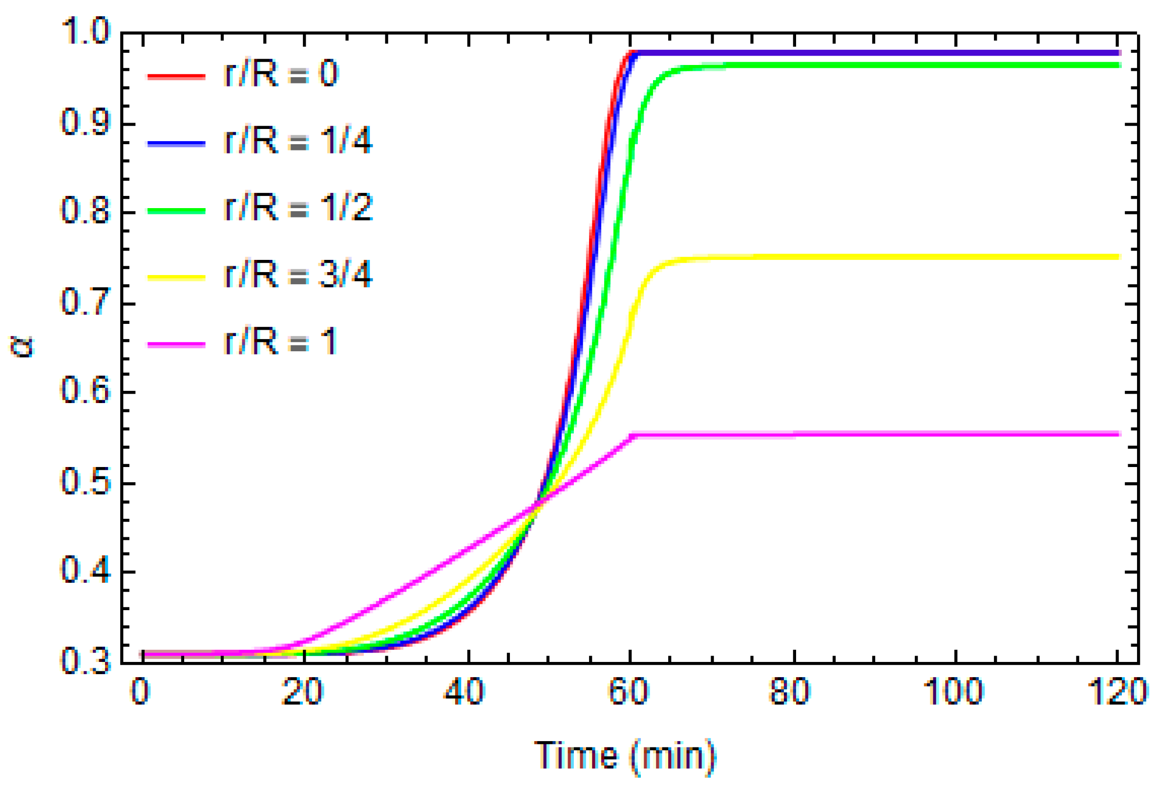
3. Results and Discussion
4. Conclusions
Author Contributions
Funding
Data Availability Statement
Conflicts of Interest
References
- Baek, J.H.; Oh, G.H.; Park, D.W.; Kawk, D.O.; Park, S.S.; Kim, H.S. Effect of cure shrinkage of epoxy molding compound on warpage behavior of semiconductor package. Mater. Sci. Semicond. Process. 2022, 148, 106758. [Google Scholar] [CrossRef]
- Dallaev, R.; Pisarenko, T.; Papež, N.; Sadovský, P.; Holcman, V. A Brief Overview on Epoxies in Electronics: Properties, Applications, and Modification. Polymers 2023, 1, 3964. [Google Scholar] [CrossRef] [PubMed]
- Jin, H.; Miller, G.M.; Pety, S.J.; Griffin, A.S.; Stradley, D.S.; Roach, D.; Sottos, N.R.; White, S.R. Fracture behavior of a self-healing, toughened epoxy adhesive. Int. J. Adhes. Adhes. 2013, 44, 157–165. [Google Scholar] [CrossRef]
- Quan, D.; Murphy, N.; Ivankovic, A. Fracture behaviour of epoxy adhesive joints modified with core-shell rubber nanoparticles. Eng. Fract. Mech. 2017, 182, 566–576. [Google Scholar] [CrossRef]
- Hao, Y.; Liu, F.; Han, E. Protection of epoxy coatings containing polyaniline modified ultra-short glass fibers. Prog. Org. Coat. 2013, 76, 571–580. [Google Scholar] [CrossRef]
- Jin, F.L.; Li, X.; Park, S.J. Synthesis and application of epoxy resins: A review. J. Ind. Eng. Chem. 2015, 29, 1–11. [Google Scholar] [CrossRef]
- Müller-Pabel, M.; Rodríguez Agudo, J.A.; Gude, M. Measuring and understanding cure-dependent viscoelastic properties of epoxy resin: A review. Polym. Test. 2022, 114, 107701. [Google Scholar] [CrossRef]
- Mahesh, V.; Joladarashi, S.; Kulkarni, S.M. A comprehensive review on material selection for polymer matrix composites subjected to impact load. Def. Technol. 2021, 17, 257–277. [Google Scholar] [CrossRef]
- Barra, G.; Guadagno, L.; Raimondo, M.; Santonicola, M.G.; Toto, E.; Vecchio Ciprioti, S. A Comprehensive Review on the Thermal Stability Assessment of Polymers and Composites for Aeronautics and Space Applications. Polymers 2023, 15, 3786. [Google Scholar] [CrossRef]
- Vidil, T.; Tournilhac, F.; Musso, S.; Robisson, A.; Leibler, L. Control of reactions and network structures of epoxy thermosets. Prog. Polym. Sci. 2016, 62, 126–179. [Google Scholar] [CrossRef]
- O’Brien, D.J.; Sottos, N.R.; White, S.R. Cure-dependent Viscoelastic Poisson’s Ratio of Epoxy. Exp. Mech. 2007, 47, 237–249. [Google Scholar] [CrossRef]
- D’Elia, R.; Sanches, L.; Des, J.M.; Michon, G. Experimental characterization and numerical modeling of a viscoelastic expandable epoxy foam: Time–temperature transformation and time–temperature equivalence diagrams. J. Appl. Polym. Sci. 2023, 140, e53929. [Google Scholar] [CrossRef]
- Courtois, A.; Hirsekorn, M.; Benavente, M.; Jaillon, A.; Marcin, L.; Ruiz, E.; Lévesque, M. Viscoelastic behavior of an epoxy resin during cure below the glass transition temperature: Characterization and modeling. J. Compos. Mater. 2018, 53, 155–171. [Google Scholar] [CrossRef]
- Eom, Y.; Hirsekorn, M.; Benavente, M.; Jaillon, A.; Marcin, L.; Ruiz, E.; Lévesque, M. Time-cure-temperature superposition for the prediction of instantaneous viscoelastic properties during cure. Polym. Eng. Sci. 2004, 40, 1281–1292. [Google Scholar] [CrossRef]
- Grassia, L.; D’Amore, A. On the interplay between viscoelasticity and structural relaxation in glassy amorphous polymers. J. Polym. Sci. B Polym. Phys. 2009, 47, 724–739. [Google Scholar] [CrossRef]
- Seregar, J.; Martin, P.J.; Menary, G.; McCourt, M.; Kearns, M. Development of warpage simulation for rotationally moulded parts and the analysis of process parameters. Polym. Eng. Sci. 2023, 64, 1144–1155. [Google Scholar] [CrossRef]
- Zarrelli, M.; Partridge, I.K.; D’Amore, A. Warpage induced in bi-material specimens: Coefficient of thermal expansion, chemical shrinkage and viscoelastic modulus evolution during cure. Compos. Part A Appl. Sci. Manuf. 2006, 37, 565–570. [Google Scholar] [CrossRef]
- Patham, B. Multiphysics simulations of cure residual stresses and springback in a thermoset resin using a viscoelastic model with cure-temperature-time superposition. J. Appl. Polym. Sci. 2012, 129, 983–998. [Google Scholar] [CrossRef]
- Parlevliet, P.P.; Bersee, H.E.N.; Beukers, A. Residual stresses in thermoplastic composites—A study of the literature—Part I: Formation of residual stresses. Compos. Part A Appl. Sci. Manuf. 2006, 37, 1847–1857. [Google Scholar] [CrossRef]
- Wu, L.F.; Zhu, J.G.; Xie, H.M. Investigation of Residual Stress in 2D Plane Weave Aramid Fibre Composite Plates Using Moiré Interferometry and Hole-Drilling Technique. Strain 2015, 51, 429–443. [Google Scholar] [CrossRef]
- Yun, H.B.; Eslami, E.; Zhou, L. Noncontact stress measurement from bare UHPC surface using Raman piezospectroscopy. J. Raman. Spectrosc. 2018, 49, 1540–1551. [Google Scholar] [CrossRef]
- Roh, H.D.; Lee, S.Y.; Jo, E.; Kim, H.; Ji, W.; Park, Y.B. Deformation and interlaminar crack propagation sensing in carbon fiber composites using electrical resistance measurement. Compos. Struct. 2019, 216, 142–150. [Google Scholar] [CrossRef]
- Rufai, O.; Chandarana, N.; Gautam, M.; Potluri, P.; Gresil, M. Cure monitoring and structural health monitoring of composites using micro-braided distributed optical fibre. Compos. Struct. 2020, 254, 112861. [Google Scholar] [CrossRef]
- Zhu, P.; Xie, X.; Sun, X.; Soto, M.A. Distributed modular temperature-strain sensor based on optical fiber embedded in laminated composites. Compos. B Eng. 2019, 168, 267–273. [Google Scholar] [CrossRef]
- Parlevliet, P.P.; Bersee, H.E.N.; Beukers, A. Residual stresses in thermoplastic composites-A study of the literature—Part II: Experimental techniques. Compos. Part A Appl. Sci. Manuf. 2007, 38, 651–665. [Google Scholar] [CrossRef]
- Chen, J.; Peng, Y.; Zhao, S. Hole-drilling method using grating rosette and Moiré interferometry. Acta Mech. Sin. 2009, 25, 389–394. [Google Scholar] [CrossRef]
- Ibrahim Mamane, A.S.; Giljean, S.; Pac, M.J.; L’Hostis, G. Optimization of the measurement of residual stresses by the incremental hole drilling method. Part I: Numerical correction of experimental errors by a configurable numerical–experimental coupling. Compos. Struct. 2022, 294, 115703. [Google Scholar] [CrossRef]
- Maiarù, M.; D’Mello, R.J.; Waas, A.M. Characterization of intralaminar strengths of virtually cured polymer matrix composites. Compos. B Eng. 2018, 149, 285–295. [Google Scholar] [CrossRef]
- Johnston, A.; Vaziri, R.; Poursartip, A. A Plane Strain Model for Process-Induced Deformation of Laminated Composite Structures. J. Compos. Mater. 2001, 35, 1435–1469. [Google Scholar] [CrossRef]
- Zhang, F.; Ye, Y.; Li, M.; Wang, H.; Cheng, L.; Wang, Q.; Ke, Y. Computational modeling of micro curing residual stress evolution and out-of-plane tensile damage behavior in fiber-reinforced composites. Compos. Struct. 2023, 322, 117370. [Google Scholar] [CrossRef]
- Liu, X.; Guan, Z.; Wang, X.; Jiang, T.; Geng, K.; Li, Z. Study on cure-induced residual stresses and spring-in deformation of L-shaped composite laminates using a simplified constitutive model considering stress relaxation. Compos. Struct. 2021, 272, 114203. [Google Scholar] [CrossRef]
- Bogetti, T.A.; Gillespie, J.W. Process-Induced Stress and Deformation in Thick-Section Thermoset Composite Laminates. J. Comp. Mater. 1992, 26, 626–660. [Google Scholar] [CrossRef]
- Kim, Y.K.; White, S.R. Stress relaxation behavior of 3501-6 epoxy resin during cure. Polym. Eng. Sci. 1996, 36, 2852–2862. [Google Scholar] [CrossRef]
- Verde, R.; D’Amore, A.; Grassia, L. A Numerical Model to Predict the Relaxation Phenomena in Thermoset Polymers and Their Effects on Residual Stress during Curing—Part I: A Theoretical Formulation and Numerical Evaluation of Relaxation Phenomena. Polymers 2024, 16, 1433. [Google Scholar] [CrossRef] [PubMed]
- D’Amore, A.; Caputo, F.; Grassia, L.; Zarelli, M. Numerical evaluation of structural relaxation-induced stresses in amorphous polymers. Compos. Part A Appl. Sci. Manuf. 2006, 37, 556–564. [Google Scholar] [CrossRef]
- Grassia, L.; D’Amore, A. Residual Stresses in Amorphous Polymers. Macromol. Symp. 2005, 228, 1–16. [Google Scholar] [CrossRef]
- Grassia, L.; D’Amore, A. Calculation of the shrinkage-induced residual stress in a viscoelastic dental restorative material. Mech Time Depend. Mater. 2012, 17, 1–13. [Google Scholar] [CrossRef]
- Goncalves, P.T.; Arteiro, A.; Rocha, N.; Pina, L. Numerical Analysis of Micro-Residual Stresses in a Carbon/Epoxy Polymer Matrix Composite during Curing Process. Polymers 2022, 14, 2653. [Google Scholar] [CrossRef]
- Shah, S.P.; Maiarù, M. Effect of Manufacturing on the Transverse Response of Polymer Matrix Composites. Polymers 2021, 13, 2491. [Google Scholar] [CrossRef]
- Bogetti, T.A.; Gillespie, J.W. Two-Dimensional Cure Simulation of Thick Thermosetting Composites. J. Compos. Mater. 1991, 25, 239–273. [Google Scholar] [CrossRef]
- Vieira de Mattos, D.F.; Huang, R.; Liechti, K.M. The effect of moisture on the nonlinearly viscoelastic behavior of an epoxy. Mech. Time Depend. Mater. 2020, 24, 435–461. [Google Scholar] [CrossRef]
- Narayanaswamy, S. A Model of Structural Relaxation in Glass. J. Am. Ceram. Soc. 1971, 54, 491–498. [Google Scholar] [CrossRef]
- Tool, A. Relation between inelastic deformability and thermal expansion of glass in its annealing range. J. Am. Ceram. Soc. 1946, 29, 240–253. [Google Scholar] [CrossRef]
- Markovsky, A.; Soules, T.F. An Efficient and Stable Algorithm for Calculating Fictive Temperatures. J. Am. Ceram. Soc. 1984, 67, c56–c57. [Google Scholar] [CrossRef]
- Zarrelli, M.; Skordos, A.A.; Partridge, I.K. Investigation of cure induced shrinkage in unreinforced epoxy resin. Plast. Rubber Compos. 2013, 31, 377–384. [Google Scholar] [CrossRef]


| A1 | 2.102 × 10⁹ | min−1 |
| A2 | −2.014 × 10⁹ | min−1 |
| A3 | 1.960 × 10⁵ | min−1 |
| ΔE1 | 8.07 × 10⁴ | J/mol |
| ΔE2 | 7.78 × 10⁴ | J/mol |
| ΔE3 | 5.66 × 10⁴ | J/mol |
| Hr | 473.16 | kJ/ Kg |
| R | 8.314 | J/Kg mol |
| ρ | 1200 | Kg/m3 |
| cp | 1260 | J/Kg K |
| k | 0.167 | W/m K |
| b1 | 284.46 |
| b2 | −47.33 |
| b3 | 239.4 |
| k4 | 8272 |
| k5 | −18,541 |
| k6 | 2780 |
| k7 | 0.833 |
| k8 | 0.0374 |
| N | τG (s) | αiG |
| 1 | 1.75 × 10⁻⁹ | 0.059 |
| 2 | 1.75 × 10⁻⁷ | 0.066 |
| 3 | 1.09 × 10⁻⁵ | 0.083 |
| 4 | 6.60 × 10⁻⁴ | 0.112 |
| 5 | 1.70 × 10⁻² | 0.154 |
| 6 | 4.76 × 10⁻¹ | 0.262 |
| 7 | 1.17 × 101 | 0.184 |
| 8 | 2.00 × 10² | 0.049 |
| 9 | 2.95 × 10⁴ | 0.025 |
| N | τM (s) | αiM |
| 1 | 1.21 × 10⁻⁶ | 0.0062 |
| 2 | 2.60 × 10⁻⁵ | 0.0072 |
| 3 | 5.60 × 10⁻⁴ | 0.0175 |
| 4 | 1.21 × 10⁻² | 0.0390 |
| 5 | 2.60 × 10⁻¹ | 0.0856 |
| 6 | 5.60 | 0.1730 |
| 7 | 1.21 × 10² | 0.2950 |
| 8 | 2.60 × 10³ | 0.298 |
| 9 | 5.60 × 10⁴ | 0.0785 |
Disclaimer/Publisher’s Note: The statements, opinions and data contained in all publications are solely those of the individual author(s) and contributor(s) and not of MDPI and/or the editor(s). MDPI and/or the editor(s) disclaim responsibility for any injury to people or property resulting from any ideas, methods, instructions or products referred to in the content. |
© 2024 by the authors. Licensee MDPI, Basel, Switzerland. This article is an open access article distributed under the terms and conditions of the Creative Commons Attribution (CC BY) license (https://creativecommons.org/licenses/by/4.0/).
Share and Cite
Verde, R.; D’Amore, A.; Grassia, L. A Numerical Model to Predict the Relaxation Phenomena in Thermoset Polymers and Their Effects on Residual Stress during Curing, Part II: Numerical Evaluation of Residual Stress. Polymers 2024, 16, 1541. https://doi.org/10.3390/polym16111541
Verde R, D’Amore A, Grassia L. A Numerical Model to Predict the Relaxation Phenomena in Thermoset Polymers and Their Effects on Residual Stress during Curing, Part II: Numerical Evaluation of Residual Stress. Polymers. 2024; 16(11):1541. https://doi.org/10.3390/polym16111541
Chicago/Turabian StyleVerde, Raffaele, Alberto D’Amore, and Luigi Grassia. 2024. "A Numerical Model to Predict the Relaxation Phenomena in Thermoset Polymers and Their Effects on Residual Stress during Curing, Part II: Numerical Evaluation of Residual Stress" Polymers 16, no. 11: 1541. https://doi.org/10.3390/polym16111541
APA StyleVerde, R., D’Amore, A., & Grassia, L. (2024). A Numerical Model to Predict the Relaxation Phenomena in Thermoset Polymers and Their Effects on Residual Stress during Curing, Part II: Numerical Evaluation of Residual Stress. Polymers, 16(11), 1541. https://doi.org/10.3390/polym16111541