
Study of Mathematical Models Describing the Thermal Decomposition of Polymers Using Numerical Methods

 , ,
, ,
Abstract
:1. Introduction
2. Methods
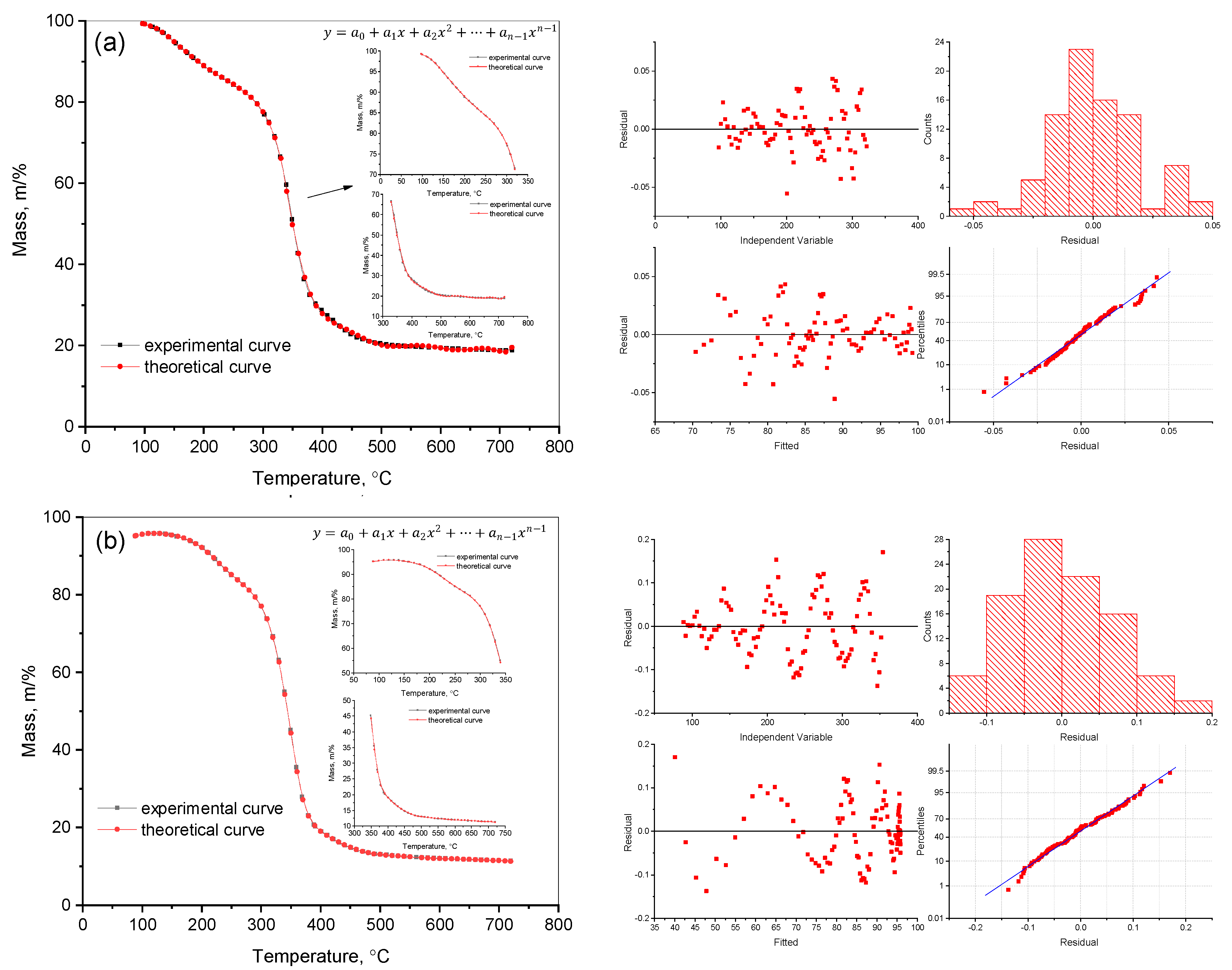
2.1. Approximation Techniques and TGA-Based Analysis
2.2. Density Functional Theory (DFT) Calculations
2.3. Methods for Solving Systems of Equations
2.3.1. Methods for Calculating Kinetic Parameters
2.3.2. Method of Least Squares
- -
- Find the partial derivatives of the function Q(b, m and Ti) to the unknowns b and m;
- -
- Set the resulting expressions equal to zero;
- -
- Solve the resulting system of two equations with two unknowns.
2.3.3. Normal Equations
2.3.4. Cholesky Factorization
2.3.5. QR Decomposition
2.3.6. Modified Gram–Schmidt
2.3.7. Singular Value Decomposition (SVD)
3. Results
3.1. Methods of Mathematical Processing of Experimental Data
- (1)
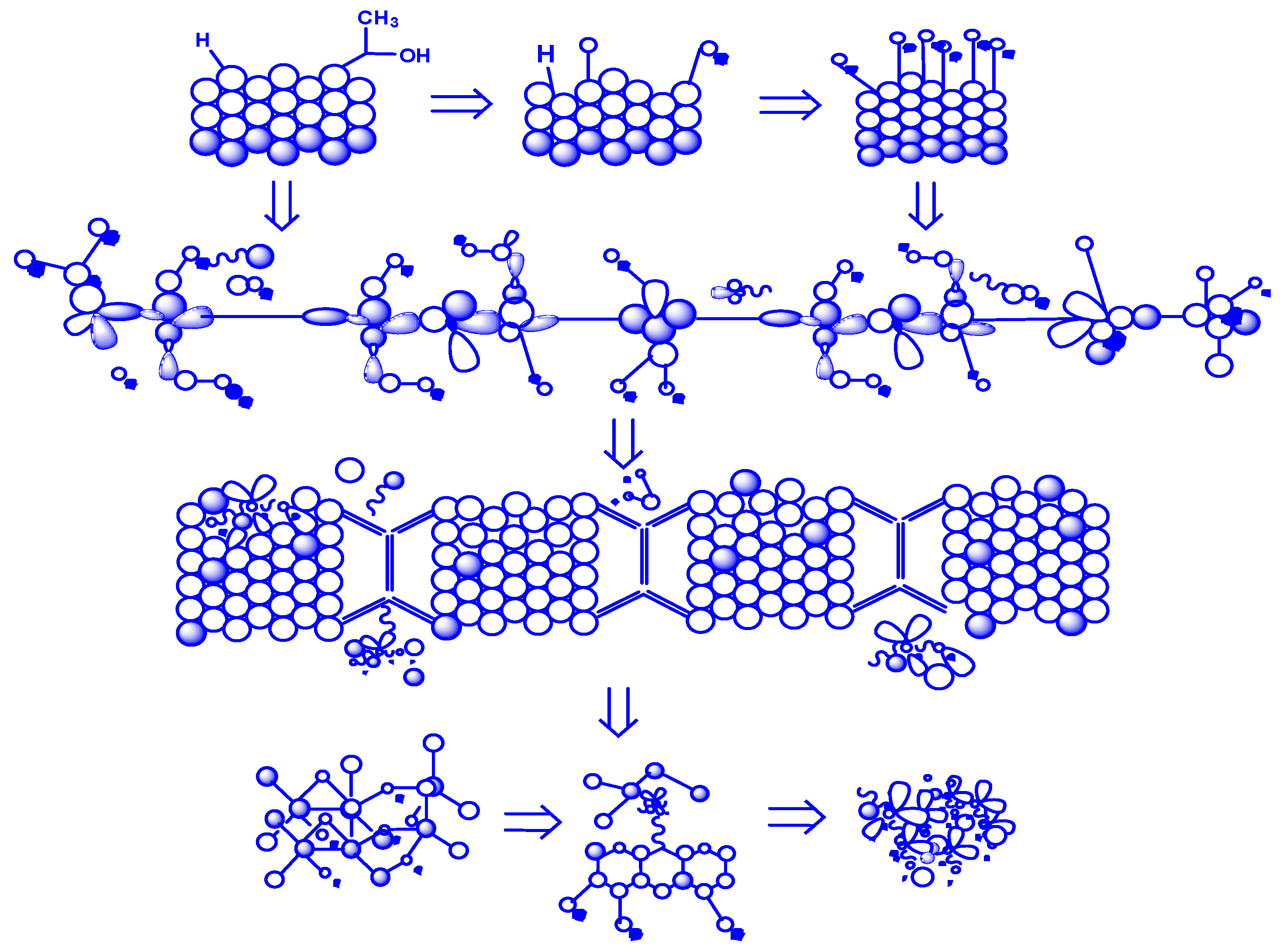
- Initiation—The initial stage, involving the rupture of weak bonds in the polymer chain, which triggers the process of technological degradation.
- (2)
- Propagation—The process in which active radicals are formed, stimulating further polymer breakdown. As a result of structural changes in the chain, degradation products begin to form.
- (3)
- Elimination—The stage in which volatile compounds, such as carbon dioxide (CO2), carbon monoxide (CO), and other small molecules, are formed.
- (4)
- Formation of Intermediate Products—During thermal degradation, cyclic and aromatic compounds are formed, which are eventually converted into solid residues.
- (5)
- Final Product—The carbonaceous residue (coke deposit) that remains after the completion of all degradation stages.
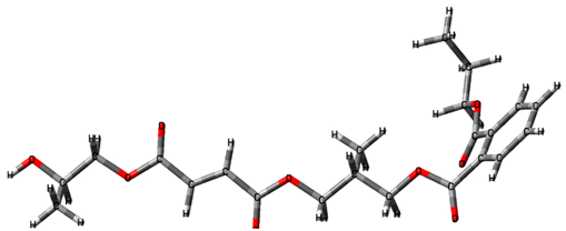
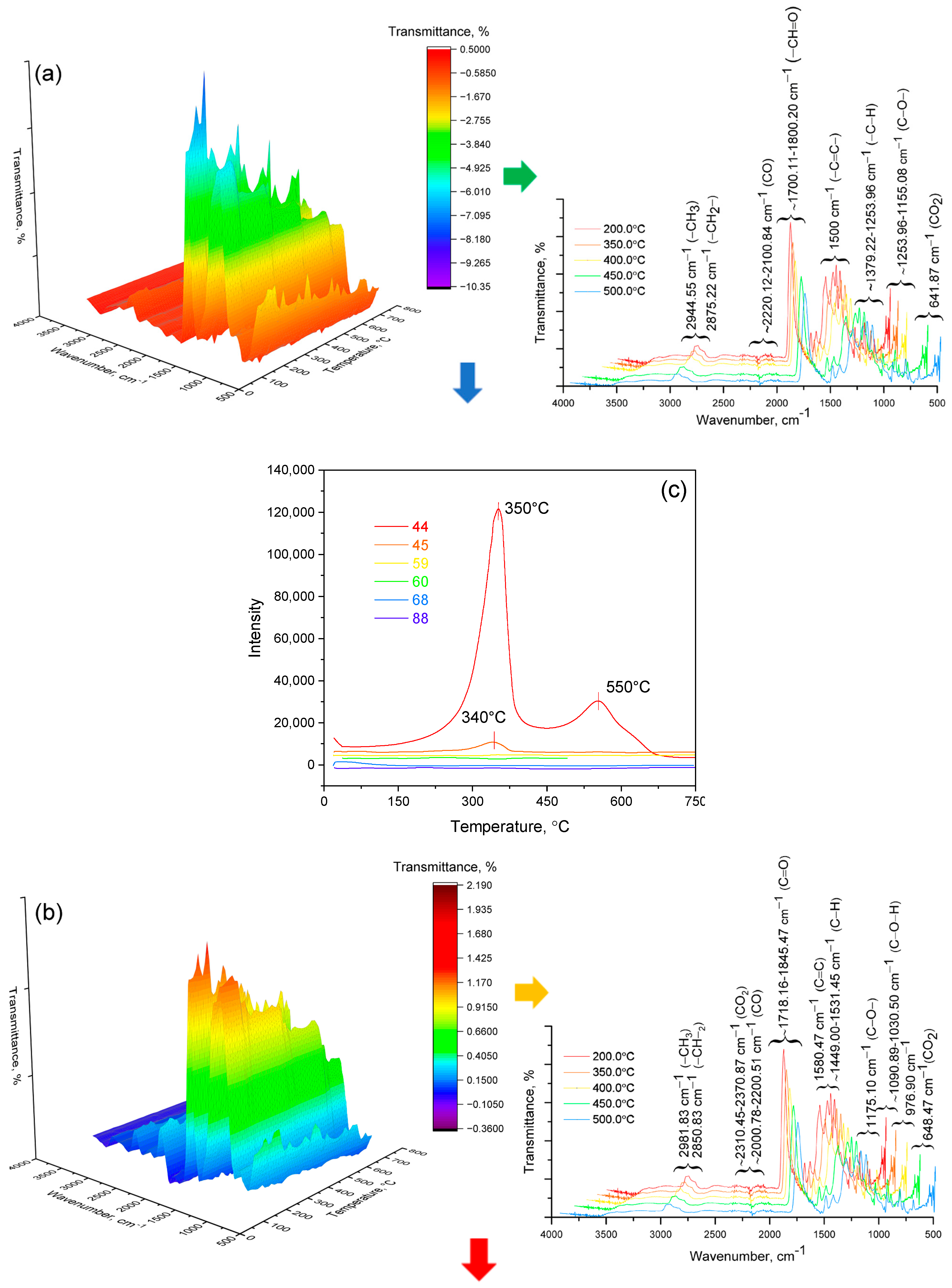
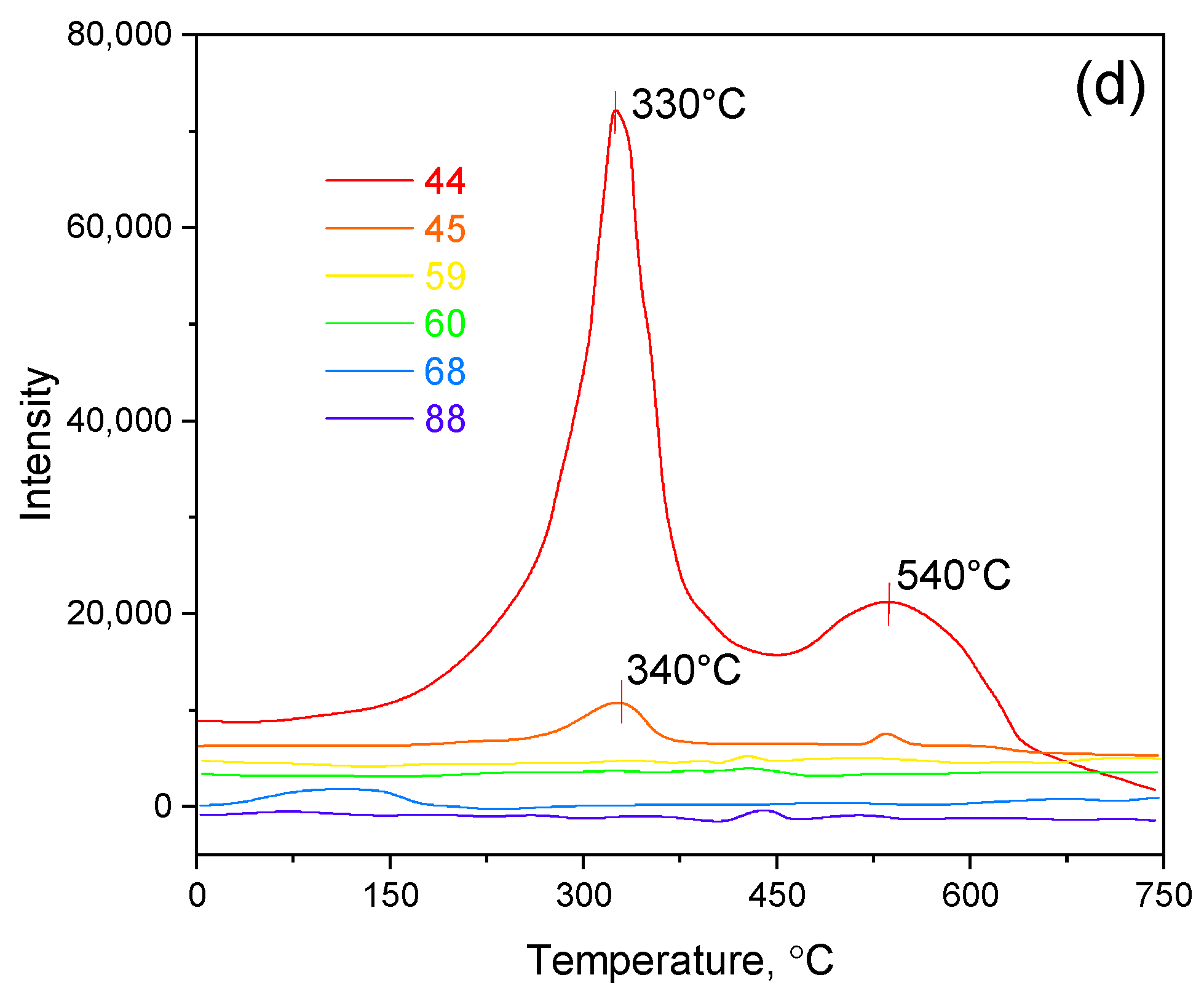
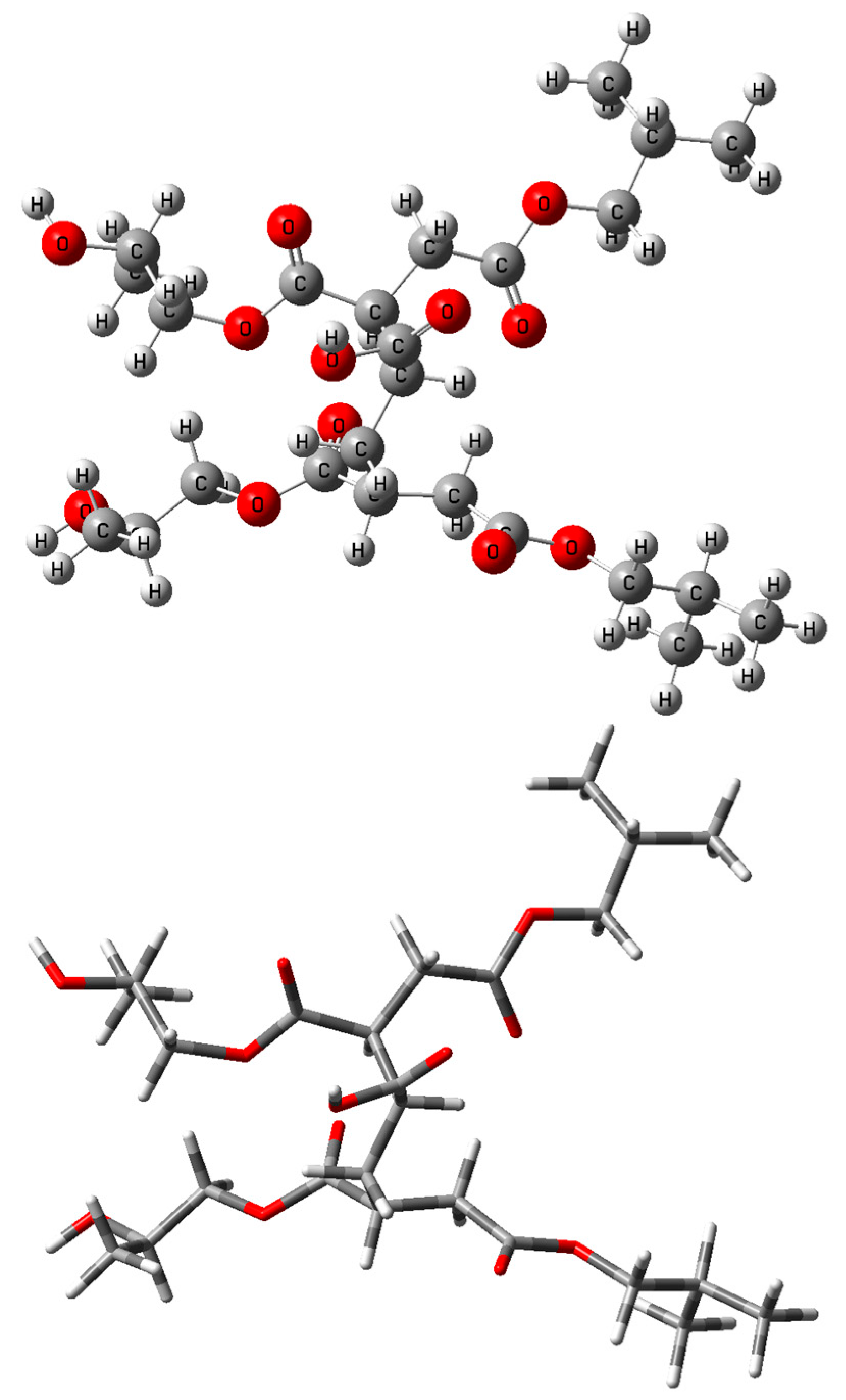
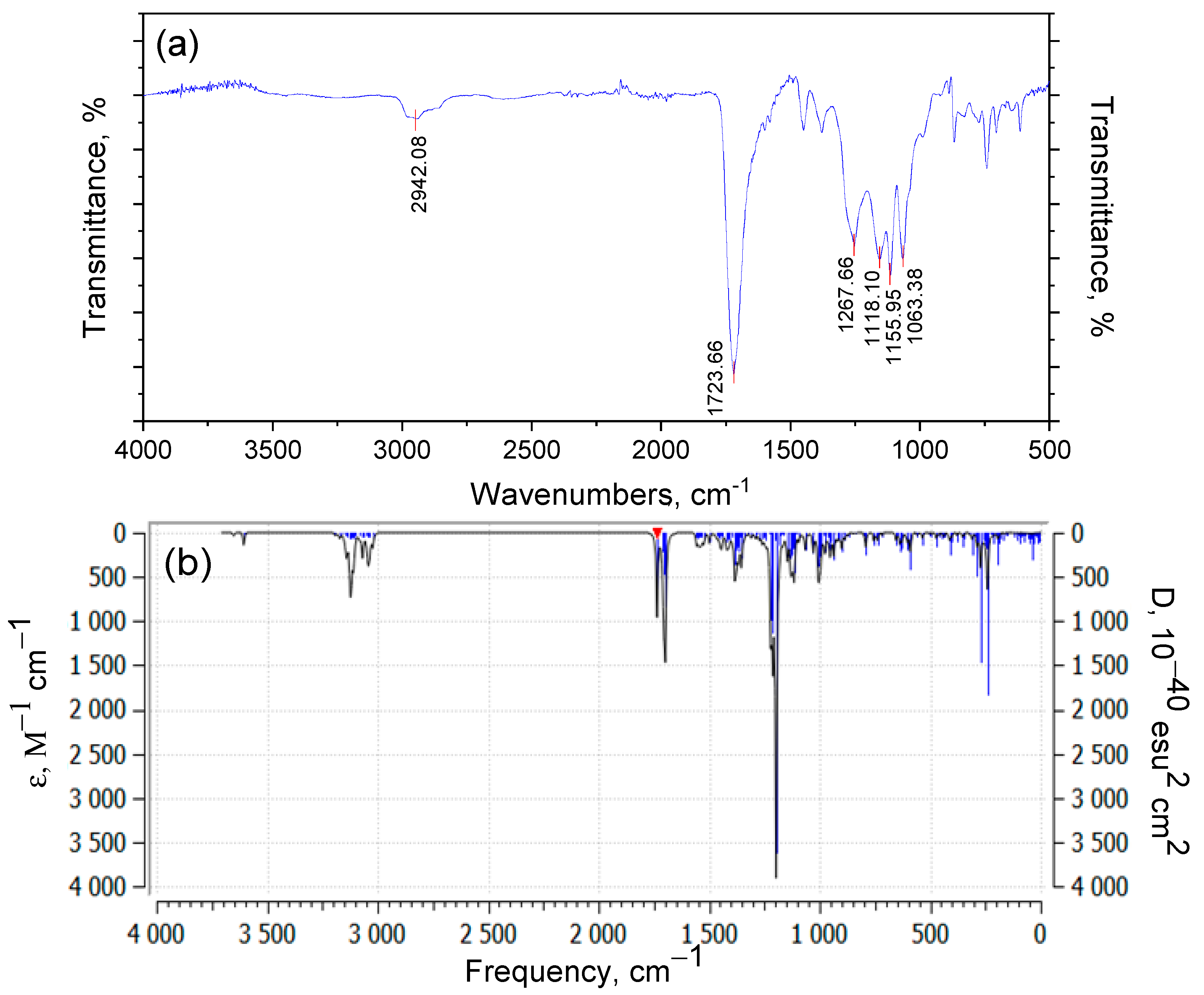
3.2. Investigation by IR Spectroscopy and Quantum Chemistry of p-PGFPh:AA
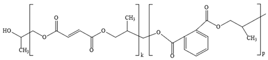
- -
- Efficient integration of the monomer into a three-dimensional crosslinked polymer matrix;
- -
- Fine-tuning of the composition for specific applications, including the grafting of biologically active fragments.
4. Conclusions
5. Patents
Supplementary Materials
Author Contributions
Funding
Institutional Review Board Statement
Data Availability Statement
Conflicts of Interest
References
- Kandelbauer, A.; Tondi, G.; Zaske, O.C.; Goodman, S.H. Unsaturated Polyesters and Vinyl Esters. In Handbook of Thermoset Plastics, 3rd ed.; Dodiuk, H., Goodman, S.H., Eds.; Elsevier: Amsterdam, The Netherlands, 2014; pp. 111–172. [Google Scholar]
- Sarsenbekova, A.Z.; Burkeyev, M.Z.; Zhumanazarova, G.M.; Kudaibergen, G.K.; Nasikhatuly, Y. The Effect of Liquid Active Media on the Character of Equilibrium Swelling of Copolymers Based on Polypropylene Fumarate Phthalate with Acrylic Acid. Eurasian J. Chem. 2023, 109, 51–58. [Google Scholar] [CrossRef]
- Taha, M.R.; Genedy, M.; Ohama, Y. Polymer Concrete Developments in the Formulation and Reinforcement of Concrete; Elsevier: Amsterdam, The Netherlands, 2019; pp. 391–408. [Google Scholar] [CrossRef]
- Benig, G.V. Unsaturated Polyesters: Structure and Properties; Elsevier: Amsterdam, The Netherlands, 1968; pp. 251–253. [Google Scholar]
- Kim, J.; Jeong, D.; Son, C.; Lee, Y.; Kim, E.; Moom, I. Synthesis & Application of Unsaturated Polyester Resins based on PET Waste. Korean J. Chem. Eng. 2007, 24, 1076–1083. [Google Scholar] [CrossRef]
- Dholakiya, B. Unsaturated Polyester Resin for Specialty Applications. Polyester 2012, 7, 167–202. [Google Scholar] [CrossRef]
- Malchiodi, B.; Siligardi, C.; Pozzi, P. Unsaturated polyester-based polymer concrete containing recycled cathode ray tube glass aggregate. J. Compos. Sci. 2022, 6, 47. [Google Scholar] [CrossRef]
- Wypych, G. Handbook of Polymers; Elsevier: Amsterdam, The Netherlands, 2022; ISBN 9781927885956. [Google Scholar]
- Arasu, P.M.; Karthikayan, A.; Venkatachalam, R. Mechanical and thermal behavior of hybrid glass/jute fiber reinforced composites with epoxy/polyester resin. Polimery 2019, 64, 504–508. [Google Scholar] [CrossRef]
- Akaluzia, R.O.; Edoziuno, F.O.; Adediran, A.A.; Odoni, B.U.; Edibo, S.; Olayanju, T.M.A. Evaluation of the effect of reinforcement particle sizes on the impact and hardness properties of hardwood charcoal particulate-polyester resin composites. Mater. Today Proc. 2021, 38, 570–577. [Google Scholar] [CrossRef]
- Abu-Jdayil, B. Unsaturated Polyester Microcomposites. In Unsaturated Polyester Resins; Sabu, T., Mahesh, H., Cintil, J.C., Eds.; Elsevier: Amsterdam, The Netherlands, 2019; pp. 67–100. [Google Scholar] [CrossRef]
- Burkeev, M.; Zhumanazarova, G.; Tazhbayev, E.; Kudaibergen, G.; Aukadieva, S.; Zhakupbekova, E. Poly(propylenefumarate phthalate)and Acrylic Acid Radical Copolymerization Constants and Parameters. Bull. Karaganda Univ. Chem Ser. 2020, 97, 68–74. [Google Scholar] [CrossRef]
- Burkeev, M.Z.; Bolatbay, A.N.; Sarsenbekova, A.Z.; Davrenbekov, S.Z.; Nasikhatuly, E. Integral Ways of Calculating the Destruction of Copolymers of Polyethylene Glycol Fumarate with Acrylic Acid. Russ. J. Phys. Chem. A 2021, 95, 2009–2013. [Google Scholar] [CrossRef]
- Burkeev, M.Z.; Tazhbaev, E.M.; Mustafin, E.S.; Fomin, V.N.; Magzumova, A.K. Method of Obtaining of Unsaturated Polyester Resin from Maleic Acid and Ethylene Glycol. Patent 31799, 26 December 2008. [Google Scholar]
- Burkeev, M.Z.; Tazhbaev, E.M.; Sarsenbekova, A.Z. Method for Producing Unsaturated Polyester Resins Based on Propylene glycol, Phthalic Anhydride and Fumaric Acid. Patent 31052, 15 April 2016. [Google Scholar]
- Kadam, V.; Jagtap, C.; Kumkale, V.; Rednam, U.; Lokhande, P.; Pathan, H. Photocatalytic Degradation of Rose Bengal Dye using Chemically Synthesized Pristine and Molybdenum doped ZnO. Eng. Sci. 2024, 28, 1077. [Google Scholar] [CrossRef]
- More, S.G.; Parveen, F.; Pathan, H.M.; Jadkar, S.R.; Gadakh, S.R. Biomolecule-Assisted Hydrothermal Synthesis of Copper Aluminium Sulfide: Application for Dye Degradation. ES Energy Environ. 2024, 25, 1209. [Google Scholar] [CrossRef]
- Sarsenbekova, A.Z.; Bolatbay, A.N.; Havlicek, D.; Issina, Z.A.; Sarsenbek, A.Z.; Kabdenova, N.A.; Kilybay, M.A. Effect of Heat Treatment on the Supramolecular Structure of Copolymers Based on Poly(propylene glycol fumarate phthalate) with Acrylic Acid. Eurasian J. Chem. 2024, 2, 61–73. [Google Scholar] [CrossRef]
- Lyulin, S.V.; Larin, S.V.; Nazarychev, V.M.; Fal’kovich, S.G.; Kenny, J.M. Multiscale computer simulation of polymer nanocomposites based on thermoplastics. Polym. Sci. Ser. C 2016, 58, 2–15. [Google Scholar] [CrossRef]
- Martin, F.; Zipse, H. Charge distribution in the water molecule−A comparison of methods. J. Comput. Chem. 2005, 26, 97–105. [Google Scholar] [CrossRef] [PubMed]
- ASTM E1582-00 (Reapproved 2016); Standard Practice for Calibration of Temperature Scale for Thermogravimetry. ASTM International: West Conshohocken, PA, USA, 2016.
- Alanazi, A.; Brown, T.; Kendell, S.; Miron, D.; Munshi, A. Time-Varying Flexible Least Squares for Thermal Desorption of Gases. Int. J. Chem. Kinet. 2013, 45, 374–386. [Google Scholar] [CrossRef]
- Koga, N.; Vyazovkin, S.; Burnham, A.; Favergeon, L.; Muravyev, N.; Pérez-Maqueda, L.; Saggese, C.; Sánchez-Jiménez, P. ICTAC Kinetics Committee recommendations for analysis of thermal decomposition kinetics. Thermochim. Acta 2023, 719, 17384. [Google Scholar] [CrossRef]
- Bau, D., III; Trefethen, L. Numerical Linear Algebra; Siam: Philadelphia, PA, USA, 1997; pp. 77–85. [Google Scholar]
- DaCosta, H.; Fan, M. Rate Constant Calculation for Thermal Reactions: Methods and Applications; Wiley: Hoboken, NJ, USA, 2012. [Google Scholar]
- Garrido, M.; Larrechi, M.; Rius, F. Multivariate curve resolution-alternating least squares and kinetic modeling applied to near-infrared data from curing reactions of epoxy resins: Mechanistic approach and estimation of kinetic rate constants. Appl. Spectrosc. 2006, 60, 174–181. [Google Scholar] [CrossRef] [PubMed]
- Gilbert, T.; Kirss, R.; Foster, N.; Davies, G. Chemistry: The Science in Context; W.W. Norton and Company: New York, NY, USA, 2004; pp. 702–761. [Google Scholar]
- Golub, G.; Van Loan, C. Matrix Computations, 4th ed.; Johns Hopkins University: Baltimore, MD, USA, 2013; pp. 76–80, 163–164, 246–250, 262–264. [Google Scholar]
- Sadun, L. Applied Linear Algebra: The Decoupling Principle, 2nd ed.; American Mathematical Society: Providence, RI, USA, 2008; pp. 143, 167–181. [Google Scholar]
- Sundberg, R. Statistical aspects on fitting the Arrhenius equation. Chemom. Intell. Lab. Syst. 1998, 41, 249–252. [Google Scholar] [CrossRef]
- Sarsenbekova, A.Z.; Zhumanazarova, G.M.; Yildirim, E.; Tazhbayev, Y.M.; Kudaibergen, G.K. RAFT agent effect on graft poly(acrylic acid) to polypropylene glycol fumarate phthalate. Chem. Pap. 2024, 78, 3831–3843. [Google Scholar] [CrossRef]
- Sarsenbekova, A.Z.; Zhumanazarova, G.M.; Tazhbayev, Y.M.; Kudaibergen, G.K.; Kabieva, S.K.; Issina, Z.A.; Kaldybayeva, A.K.; Mukabylova, A.O.; Kilybay, M.A. Research the Thermal Decomposition Processes of Copolymers Based on Polypropyleneglycolfumaratephthalate with Acrylic Acid. Polymers 2023, 15, 1725. [Google Scholar] [CrossRef] [PubMed]
- Frisch, M.J.; Trucks, G.W.; Schlegel, H.B.; Scuseria, G.E.; Robb, M.A.; Cheeseman, J.R.; Scalmani, G.; Barone, V.; Petersson, G.A.; Nakatsuji, H.; et al. Gaussian 16, Revision A.03; Gaussian Inc.: Wallingford, CT, USA, 2016. [Google Scholar]


| Wavenumber of Experimental Peak (cm−1) | Calculated Wavenumber (cm−1) | Vibrational Assignment |
|---|---|---|
| 3535 | 3753 | Stretching vibrations of free OH groups |
| 2980–2942 | 3020–2950 | C–H stretching vibrations of CH3, CH2, and phenyl groups |
| 2355 | — | Atmospheric CO2 or trace impurities |
| 1724–1723 | 1735–1700 | C=O stretching modes in esters and carboxylic acids |
| 1637, 1450 | 1656, 1491 | Aromatic and C=C deformation modes |
| 1268, 1118, 1063 | 1270–1050 | CH2 and CH3 deformation vibrations, and ring mode vibrations |
| Sample | Cholesky Decomposition | Normal Equations | Singular Value Decomposition | QR Decomposition | ||||
|---|---|---|---|---|---|---|---|---|
| Ea (kJ mol−1) ±SD | A·108, (min−1) ±SD | Ea (kJ mol−1) ±SD | A·108, (min−1) ±SD | Ea (kJ mol−1) ±SD | A·108, (min−1) ±SD | Ea (kJ mol−1) ±SD | A·108, (min−1) ±SD | |
| EXPERIMENTAL DATA | ||||||||
| Nitrogen | ||||||||
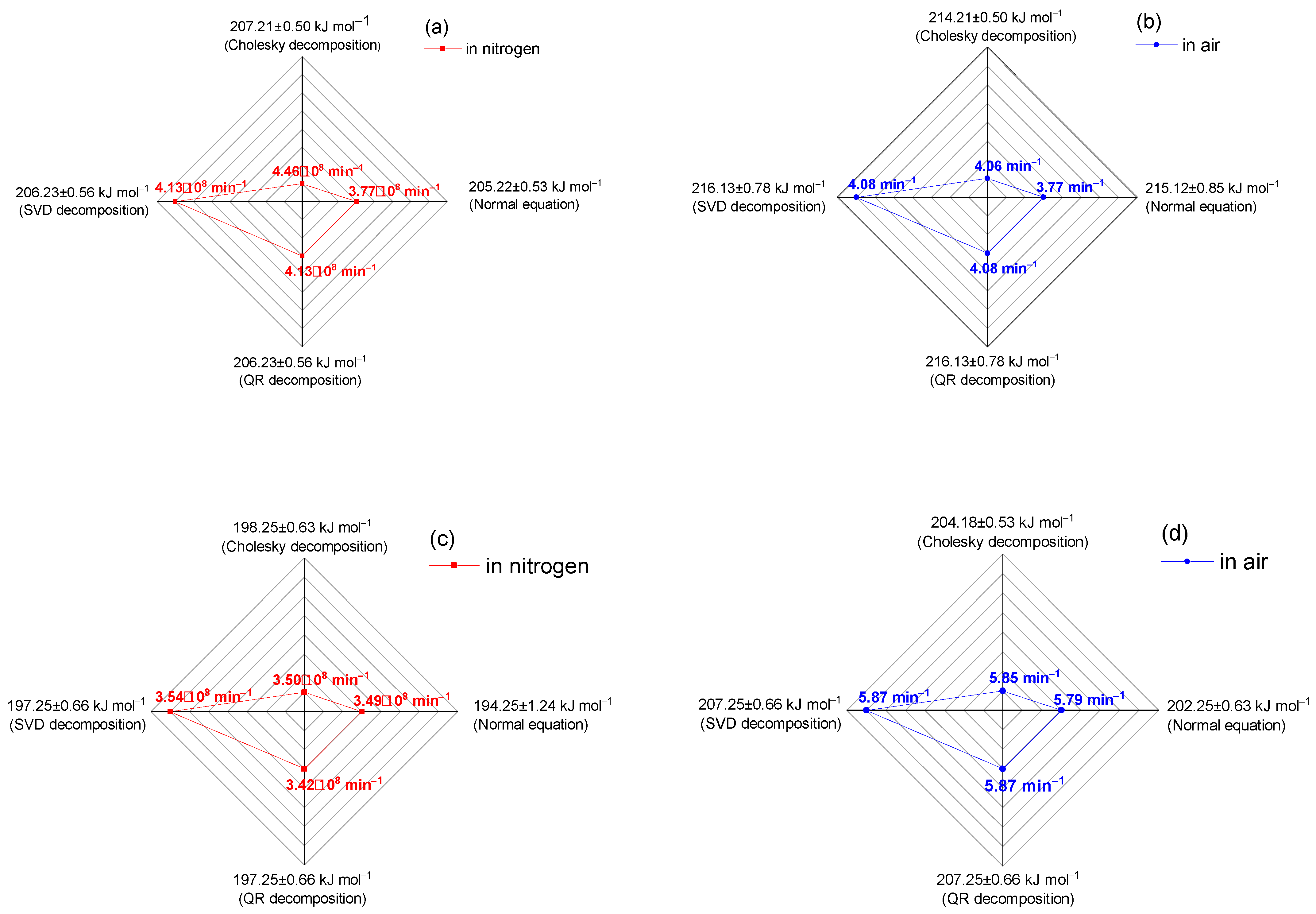
| 6.77:93.23 | 207.21 ±0.50 | 4.46 ±0.26 | 205.22 ±0.53 | 3.77 ±0.30 | 206.23 ±0.56 | 4.13 ±0.13 | 206.23 ±0.56 | 4.13 ±0.13 |
| 86.67:13.33 | 198.25 ±0.63 | 3.50 ±0.50 | 194.25 ±1.24 | 3.49 ±0.38 | 197.25 ±0.66 | 3.54 ±0.10 | 197.25 ±0.66 | 3.42 ±0.13 |
| Air | ||||||||
| 6.77:93.23 | 214.21 ±0.50 | 4.06 ±0.29 | 215.12 ±0.85 | 3.77 ±0.25 | 216.13 ±0.78 | 4.08 ±0.05 | 216.13 ±0.78 | 4.08 ±0.05 |
| 86.67:13.33 | 204.18 ±0.53 | 5.85 ±0.15 | 202.25 ±0.63 | 5.79 ±0.30 | 207.25 ±0.66 | 5.87 ±0.05 | 207.25 ±0.66 | 5.87 ±0.05 |
| THEORETICAL DATA | ||||||||
| 6.77:93.23 | 196.98 ±0.25 | 1.90 ±0.34 | 194.98 ±0.25 | 1.90 ±0.34 | 195.98 ±0.25 | 1.90 ±0.34 | 195.98 ±0.25 | 1.90 ±0.34 |
| 86.67:13.33 | 171.20 ±0.47 | 4.83 ±0.75 | 170.20 ±0.47 | 4.83 ±0.75 | 170.17 ±0.47 | 4.83 ±0.75 | 170.20 ±0.47 | 4.83 ±0.75 |
Disclaimer/Publisher’s Note: The statements, opinions and data contained in all publications are solely those of the individual author(s) and contributor(s) and not of MDPI and/or the editor(s). MDPI and/or the editor(s) disclaim responsibility for any injury to people or property resulting from any ideas, methods, instructions or products referred to in the content. |
© 2025 by the authors. Licensee MDPI, Basel, Switzerland. This article is an open access article distributed under the terms and conditions of the Creative Commons Attribution (CC BY) license (https://creativecommons.org/licenses/by/4.0/).
Share and Cite
Zhumanazarova, G.M.; Sarsenbekova, A.Z.; Abulyaissova, L.K.; Figurinene, I.V.; Zhaslan, R.K.; Makhmutova, A.S.; Sotchenko, R.K.; Aikynbayeva, G.M.; Hranicek, J. Study of Mathematical Models Describing the Thermal Decomposition of Polymers Using Numerical Methods. Polymers 2025, 17, 1197. https://doi.org/10.3390/polym17091197
Zhumanazarova GM, Sarsenbekova AZ, Abulyaissova LK, Figurinene IV, Zhaslan RK, Makhmutova AS, Sotchenko RK, Aikynbayeva GM, Hranicek J. Study of Mathematical Models Describing the Thermal Decomposition of Polymers Using Numerical Methods. Polymers. 2025; 17(9):1197. https://doi.org/10.3390/polym17091197
Chicago/Turabian StyleZhumanazarova, Gaziza M., Akmaral Zh. Sarsenbekova, Lyazzat K. Abulyaissova, Irina V. Figurinene, Rymgul K. Zhaslan, Almagul S. Makhmutova, Raissa K. Sotchenko, Gulzat M. Aikynbayeva, and Jakub Hranicek. 2025. "Study of Mathematical Models Describing the Thermal Decomposition of Polymers Using Numerical Methods" Polymers 17, no. 9: 1197. https://doi.org/10.3390/polym17091197
APA StyleZhumanazarova, G. M., Sarsenbekova, A. Z., Abulyaissova, L. K., Figurinene, I. V., Zhaslan, R. K., Makhmutova, A. S., Sotchenko, R. K., Aikynbayeva, G. M., & Hranicek, J. (2025). Study of Mathematical Models Describing the Thermal Decomposition of Polymers Using Numerical Methods. Polymers, 17(9), 1197. https://doi.org/10.3390/polym17091197