Abstract
Nitrogen fertilization is the most critical agronomic input affecting barley production and farm profitability. The strict quality requirements for malting barley are challenging to achieve for farmers. In addition, soil variability and weather conditions can affect barley yield and quality. Thus, the objectives of this study are to (a) quantify the variability of soil properties, and (b) use spatial data in a crop simulation model, quantifying the impacts of climate−soil interactions on the barley crop yield and grain quality. Based on historical yield maps, a commercial field was divided into different yield stability zone levels. The Decision Support System for Agrotechnology Transfer model was used to evaluate soil and crop spatial data. The bulk density affected the soil water content and soil mineral N and hence the crop-growing conditions in each yield stability zone. Our observed and simulated results showed that 120 kg N ha−1 is the optimal rate to increase grain yield while still keeping within the grain N% requirements for malting quality. This study shows the great value of integrating crop modeling with on−farm experimental data for improving understanding of the factors which affect site−specific N fertilization of barley.
1. Introduction
The biggest challenge facing agricultural production would be to produce more food on less land, reducing the impact of any agronomic practice and the issues caused by changing climate [1,2,3,4]. One of the most important crops in Scottish agriculture, from an agronomic and economic point of view, is barley (Hordeum vulgare L). Barley is among the oldest cultivated plants in the world, growing at very different latitudes [5], and in Scotland, its production is being mainly used in malting for the production of whisky; in fact, ~60% of the produced barley is used for malting and ~40% for animal feed [6]. From a practical point of view, stakeholders are interested in both production and quality, and therefore, agronomic factors, such as sowing time, fertilizer amount, and plant density, can be adjusted to improve both production and quality [1]. One of the most critical agronomic inputs is the application of nitrogen (N) fertilizer. Overall, N requirements are lower for spring barley than winter-sown barley due to the lower potential yield of spring barley than winter crops. Likewise, barley for malting allows a grain–N% of less than 1.85% [6]. The optimization of nutrient management for yield and quality are affected by soil variability and climatic conditions, especially at the end of the season [1,2,7]. In addition, given the challenge of matching N supply with the plant N demand, nitrate leaching from agricultural land is a significant issue in many areas of Scotland. The European Union addressed such a problem by defining nitrate-vulnerable zones and thereby regulating N inputs [8]. In Scotland, farmers observe the EU regulation by regulating the amount of N applications.
Site-specific N management offers a possibility to optimize the environmental vs. economic trade−off [9]. However, in many agricultural systems, the adoption of site-specific management has been lower than expected because of technological and socio-economic challenges [10]. The amount of N applied within a field may vary spatially and temporally among years. Several factors affecting this variability makes the spatial−temporal management of N challenging [9]. In a given field, the optimal amount of fertilizer should consider site-specific soil properties, current seasonal crop growing conditions, and their interactions [7,11]. While the spatial variability of crop growth and yield can be quantified routinely with different tools (e.g., remote sensing or proximal sensing), the temporal variability has not received the right amount of attention [12]. Temporal variability of crop growth and yield is an important component that influences agronomic decision making. Because climatic conditions dynamically interact with soil properties, the crop growth/nutrient uptake is not easy to predict. Crop simulation models (CSMs) can be used to take into account the impacts of inter-annual weather on the soil−plant−atmosphere system [13]. CSMs simulate the impacts of temporal interactions of water and N on crop growth and development as affected by weather and agronomic management [13]. CSMs have been used in a variety of cropping systems and environmental conditions, but its application to quantify spatial and temporal variability on yield is limited [9,14]. The objectives of this study are to (a) quantify the variability of soil properties across the field, and (b) evaluate how crop simulation can be used with spatial input to quantify the impacts of climate−soil interactions on the malting quality of the cultivated barley.
2. Materials and Methods
Observations were collected from a single field on a commercial farm (11 ha; 56°33’ N 3°16’ W; 50 m a.s.l.) in Scotland. The soil texture was a loam, and the soil was classified according to the Balrownie series [15]. The cultivar considered for the study was the spring barley cv. Concerto (two-row cultivar, LGseeds, Limagrain, Rothwel, UK), which is one of the most common spring barley varieties grown in Scotland. The crop was sown on 12 April 2018 at 350 plants m−2. Fertilization was uniformly distributed after emergence on 1 May 2018. Compound fertilizer containing N was applied for a total of 120 kg N ha−1 (YaraMila SULPHUR CUT, 22−4−14+7.5 SO3).
The commercial farm used a combine harvester-mounted grain yield monitor and had collected yield data from the six previous years. Historical yield maps were created to establish management zones, which were defined as sub−areas within the field. It was thought that these zones had similar yield-limiting factors and, therefore, can be potentially managed in a similar way [10,16]. In this study, the management zones were calculated by using a recently published method by [17,18]. Using this approach, three stable zones were defined as the high yield stable zone (HYZ), the medium yield stable zone (MYZ), and the low yield stable zone (LYZ); in addition, one unstable yield zone (UYZ) was identified (Figure 1). The stable zones refer to yield levels that are likely to be stable in time, either at a lower or higher yield level; while the unstable zone is an area that produced contrasting levels of yield over time. Grain yields were first standardized. Then, for every pixel, the mean (μ) and the standard deviation (σ) across all the years were calculated. Subsequently, each pixel was considered as stable if σ < 0.75 and unstable if σ ≥ 0.75. In addition, it was defined as low−yielding if μ < 0 and high−yielding if μ ≥ 0 [18].

Figure 1.
Management zones defined by overlaying six years of yield maps from the commercial farm. The blue zone represents the high yield stable zone (HYZ), the green zone represents the medium yield stable zone (MYZ), the yellow zone represents the low yield stable zone (LYZ), while the red zone represents the unstable yield zone (UYZ). The open circles represent the points where soil and plant samples were made.
In each zone, a transect was designed and the corresponding points recorded using a Trimble Juno 5 Hand−held GPS. These georeferenced points were used to collect all the soil and plant samples characterized in the present study, as thereafter described. At each point, the soil was sampled at three depths (0–0.30; 0.30–0.60; 0.60–0.90 m) one month before sowing. Those samples were analyzed for bulk density only up to 60 cm, while soil texture, mineral N, P, K, cation exchange capacity (CEC), organic matter, and water content were determined for all collected samples. One day before sowing, soil samples were collected to determine soil water content and soil mineral N. Subsequently, the soil was sampled for mineral N and soil water content on three occasions: (i) three weeks after N fertilization (23 May 2018), (ii) at flowering (20 June 2018), and (iii) at harvest (16 August 2018). On the same sample times, one square meter of the crop was sampled in each georeferenced point for aboveground biomass and crop N%. At harvest, the grain yield and grain N% were determined. All soil and plant tissue chemical analyses, except the grain N%, were made at the Yara Commercial Laboratory. The grain N% was measured with a NIR instrument (Infratec 1241 Grain Analyzer; Foss Tecator, Höganäs, Sweden). Soil water content was determined by weighing 40 g of soil sample and oven-dried at 105 °C for 48 h [19]. Plant biomass was oven−dried at 60°C until constant weight and weighted. The samples collected at harvest were used to determine the straw biomass, grain yield, grain N%. Using a MARVIN grain analyzer (GTA Sensorik GmbH, Neubrandenburg, Germany), the seed weight and thousand-grain weight (TGW) were determined.
A weather station to collect the most important climatic data was installed on the farm in 2018, recording daily rainfall (mm), solar radiation (MJ m−2 d−1), and air temperature (°C). In addition, 36 years of historical weather data (1980–2017) were obtained from the NASA−Power website [20].
The Decision Support System for Agrotechnology Transfer (DSSAT) v.4.7 was adopted as the crop simulation model [13]; in particular, the barley crop model was used (CSM−Barley). The crop model needed as input daily weather data (such as daily solar radiation, daily minimum and maximum air temperature, and rainfall), soil data (such as texture, organic matter, and bulk density), management factors such as sowing date, sowing density, fertilization details, and cultivar parameters (like phenology, growth and development) that define the type of crop (e.g., maize or wheat), specifying the growth and development coefficients. The spring barley cv. Concerto had been calibrated and evaluated in Scotland at different levels of resolutions, from field trials to a transect of farms across Scotland, and to the whole barley growing area of Scotland [1,7]. Consequently, no calibration of crop coefficients was needed. Two important inputs of the crop model that have a significant impact on simulated results are the initial soil water content and soil mineral N. These inputs were available for this study, as well as other soil chemical and physical properties, and all these data were used for model evaluation. DSSAT simulated the water−balance utilizing Ritchie’s approach [21], while crop growth and development were simulated following the approach of the CERES model [13]. Crop water stress was calculated by matching the potential crop transpiration (demand) and potential root water uptake (uptake) or plant extractable water [13,21]. Crop N uptake was simulated, comparing the potential supply of N from the soil and the demand of the crop for N [22]. The crop N demand was also divided into two components: (i) a “deficiency” demand, an amount of N that is needed to convert the actual N concentration to the critical N concentration, and (ii) new growth demand. The accumulation rate of N in grains is a function of air temperature and soil moisture because, as soil moisture decreases, grain N concentration rises as a result of the lowered dilution of N in the grain assimilate [13,22].
The DSSAT crop model was set to run a number of “what−if” simulation scenarios [9,23,24]. The model was run in each management zone following the approach of Basso et al. [24], using an incremental amount of N fertilizer (0, 60, 120 N-farmers’ practice, 180 N). The model simulated yield and cumulative N leaching from sowing to harvest, and mineral soil N at harvest. The cumulative probability function of simulated yield and cumulative N leaching was calculated following the approach of Wallach and Rivington [25].
The simulated and observed values were evaluated using the root mean square error that is calculated as follows:
where yi are the observations, the simulations, and n is the number of comparisons. Another indicator used to evaluate the crop model and the observed data was the Wilmott index of agreement (D-Index), which ranges from 0 (poor fit) and 1 (indicating a good fit). The D-Index is used as an explanatory measure of the goodness of fit and has been used as a cross−comparison method between models [26,27].
where is the mean of the observed values.
3. Results
3.1. Observed Data
The growing season weather data for 2018 showed an average value of maximum air temperature (15 °C) higher than long-term (1984–2017) average (13 °C). It was also a dry year, with a cumulative rainfall amount of 170 mm against the long−term average of 300 mm (Figure 2a,b). In particular, the period between May and July 2018, there was only 88 mm of rainfall (Figure 2a).

Figure 2.
Daily pattern of air maximum (full black line) and minimum (dotted black line) temperature, and rainfall (grey bars) for (a) the 2018 growing season and (b) for the mean values of the growing seasons from 1984 to 2017, as obtained from NASA−Power [20].
Soil texture varied between the different zones of the field and at different depths. For the 0–30 cm layer, the clay content was low for all zones with a mean value of about 13% (Figure 3). Sand content showed the highest percentage and the highest variability between the zones in the first soil layer, with the MYZ (green boxplot) showing a range of values between 42% and 63% (Figure 3). For all the zones, the percentage of sand decreased with depth while the percentage of clay increased.

Figure 3.
Boxplot of the soil texture for the high yield stable zone (H; blue box), medium yield stable zone (M; green box), low yield stable zone (L; yellow box), and unstable yield zone (U; red box) for three soil depth intervals (0–30, 30–60 and 60–90 cm). The color of the boxplots correspond to the zones shown in Figure 1. The spread of the plot represents the points collected in each zone. For each boxplot, the end of the vertical line represents, from top to the bottom, the 10th percentile and the 90th percentile. The horizontal line of the box, from the top to the bottom represents the 25th, median, and 75th percentile, respectively.
The time−series of the volumetric soil water content and mineral N content is shown in Figure 4. The volumetric soil water content, for the first 30 cm, decreased from the per-sowing/sowing period (0.28 cm3 cm−3) to flowering (0.18 cm3 cm−3), but increased between June and August (0.27 cm3 cm−3; Figure 4a). The decrease of the volumetric soil water content corresponded to the period of little or no rainfall (Figure 2a). In comparison, the soil mineral N content increased from 20 kg N ha−1 prior sowing to an average of 80 kg N ha−1 at flowering when the volumetric soil water content was the least (Figure 4a). At the soil depth of 30−60 cm, the volumetric soil water content and the soil N showed a similar pattern of first layer (Figure 4b). The main difference in volumetric soil water and soil mineral N between the zones was observed at flowering, when the drier conditions exposed the different features of the zones. For example, the LYZ (yellow line) showed greater volumetric soil–water content than the other zones at flowering with about 0.20 cm3 cm−3 while the other zones showed values of about 0.18 cm3 cm−3 (Figure 4). Soil mineral N was different between the zones and the soil depths. At flowering, the LYZ had the greatest soil mineral N content (109 kg N ha−1) at 0−30 cm depth (Figure 4a), while at 30–60 cm, the UYZ had the most soil mineral N content (180 kg N ha−1) (Figure 4b).

Figure 4.
Time-series of the volumetric soil water content (cm3 cm−3) (full line and circle) and soil mineral nitrogen (kg N ha−1) (dotted line and diamond) for the high yield stable zone (HYZ, blue), medium yield stable zone (MYZ, green), low yield stable zone (LYZ, yellow), and unstable zone (UYZ, red) for two depths (a) 0–30 and (b) 30–60 cm.
The soil bulk density differed between the management zones, with average values ranging between 1.65 g cm−3 for the UYZ and 1.72 g cm−3 for the LYZ for the first 30 cm (Figure 5). The mean values increased for all the zones for the 30–60 cm depth interval, and the LYZ had the greatest bulk density (1.79 g cm−3; Figure 5).
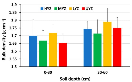
Figure 5.
Soil bulk density (g cm−3) at 0−30 and 30–60 cm for the high yield stable zone (HYZ, blue bar), medium yield stable zone (MYZ, green bar), low yield stable zone (LYZ, yellow bar), and unstable yield zone (UYZ, red bar). The error bars represent the standard deviations of the transects within each zone.
The results of the other soil chemical analyses were less variable. For instance, the soil cation exchange capacity ranged between 7.5 and 10 meq/ 100 g (Figure 6). Soil phosphorous (P) had the most variability between the management zones. The UYZ (red boxplot) had a similar mean soil P value as the other zones for the 0–30 cm depth; however, the soil P in this zone was much smaller for the two lowest depths in the soil profile (Figure 6). None of the zones were P-deficient and, in fact, the P in the topsoil (0–30 cm; Figure 6) was at Index 2 or greater (according to RB209 [28]) for all yield stability zones. For soil Ca, there was little difference between the management zones for the 0−30 cm depth, but in the 60–90 cm depth range, the HYZ was much less than the other zones (mean values were approximately 1100 ppm; Figure 6). The soil pH values were within the optimal range for barley production with mean values ranging between 6.0 and 6.6 across the different zones and depths (Figure 6).

Figure 6.
Boxplot of the soil chemical cation exchange capacity (CEC), soil phosphorous (P), soil calcium, and soil pH for the high yield stable zone (H; blue box), medium yield stable zone (M; green box), low yield stable zone (L; yellow box), and unstable yield zone (U; red box) for three soil profiles (0–30, 30–60 and 60–90 cm). The color of the boxplots correspond to the areas of Figure 1. The spread of the plot represents the points collected in each zone. For each boxplot, the end of the vertical line represents, from top to the bottom, the 10th percentile and the 90th percentile. The horizontal line of the box, from the top to the bottom, represents the 25th, median, and 75th percentile, respectively.
3.2. Simulated Volumetric Soil Water Content, Crop Biomass, and Grain Yield
The results of the model evaluation are shown in Figure 7. The volumetric soil water content was well simulated (R2 = 0.78) at different dates, with an RMSE of 0.034% and a D-Index of 0.99 (Figure 7a). The aboveground biomass at harvest had values of RMSE of 972 kg DM ha−1 and a D-Index of 0.99, with a slight underestimation at higher values of biomass (Figure 7b). The grain yield (R2 = 0.72) showed an RMSE of 601 kg DM ha−1 and a D-Index of 0.99 (Figure 7c). Soil N was simulated with an RMSE of 14.5 kg N ha−1 and a D-Index of 0.99 (Figure 7d).

Figure 7.
Observed vs. simulated data for (a) volumetric soil water content (cm3 cm−3); (b) aboveground biomass (kg DM ha−1) at harvest; (c) grain yield (kg DM ha−1); and (d) soil nitrogen (kg N ha−1) for the high yield stable zone (HYZ, blue dots), medium yield stable zone (MYZ, green dots), low yield stable zone (LYZ, yellow dots), and unstable yield zone (UYZ, red dots).
3.3. Long Term Simulations of Grain Yield According to Four Different N Fertilizer Rates
The results of the long-term simulations showed that, at low N fertilization, the different zones responded in divergent ways (Figure 8). At 0 N, the HYZ was the highest yielding zone with a mean yield of 3200 kg DM ha−1, while the UYZ showed a variable in terms of yield response with low yield values close to the LYZ (1490 kg DM ha−1) and also greater yield values close to the HYZ (4641 kg DM ha−1; Figure 8a). At higher levels of N fertilization (e.g., at 180 N; Figure 8d), the differences between the zones decreased, but the HYZ was always the most productive zone in terms of simulated yield and the LYZ the lowest (Figure 8b–c). The range between the highest and lowest yield may be due to climate variability at different N levels. The spread in simulated yield increased at the greatest N levels. The lowest yields were, across the zones, about 2000, 3900, 4000, 4100 kg DM ha−1 for the 0, 60, 120, and 180 N, respectively (Figure 8). However, the upper limit was only 4000 kg DM ha−1 for the 0 N, 6300 kg DM ha−1 for the 60 N, 8300 kg DM ha−1 for the 120 N, and 10000 kg DM ha−1 for the 180 N (Figure 8).

Figure 8.
Cumulative probability of the simulated yield using long-term weather data for the high yield stable zone (HYZ, blue line), medium yield stable zone (MYZ, green line), low yield stable zone (LYZ, yellow line), and unstable yield zone (UYZ, red line) for simulation run with (a) no nitrogen (0 N); (b) 60 kg N ha−1 (60 N); (c) 120 kg N ha−1 (120 N); and (d) 180 kg N ha−1 (180 N).
Figure 9 shows the relationship between simulated yield and simulated grain N at different N fertilization levels, overlayed with the benchmark for malting quality in terms of optimal grain N level (dash−dotted line) and maximum level above which no premium is paid [6]. At 60 N, most simulated values were below the optimal grain N%. A large proportion of the values for the 120 N were close to or above the optimal amount of grain N%, except for a few sample points, which correspond to years of low simulated yields Figure 8c and Figure 9c). At 180 N, the highest yield achieved meant that the grain N% accumulated was mostly above the maximum N%, and no premium is paid (Figure 9d).
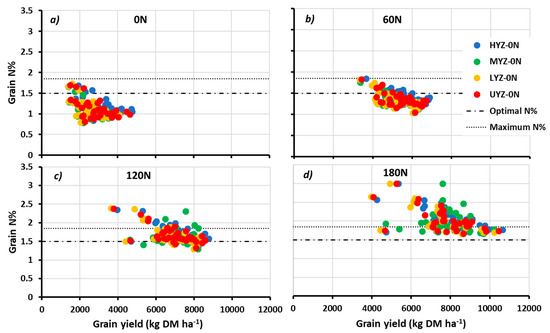
Figure 9.
The relationship between simulated yield and simulated grain N at different N fertilization levels ((a) no nitrogen (0 N); (b) 60 kg N ha−1 (60 N); (c) 120 kg N ha−1 (120 N); and (d) 180 kg N ha−1 (180 N)), overlayed with the benchmark provided for malting quality in terms of optimal grain N level (dash−dotted line) and maximum level above which no premium is paid (dotted line). Benchmark values are according to the UK malt industry [6].
4. Discussion
There was a large degree of variability within the field, with three stable zones and one unstable zone being identified within the field as the result of overlaying six years of yield maps. Among the soil factors impacting the performance of the crop growth, the soil texture and bulk density at depths below 30 cm had an important impact in terms of the distribution of soil water and soil mineral N. For example, the LYZ had very compacted layers (with values of 1.8 g cm−3), but the other management zones had smaller bulk density values. Bulk density is a dynamic soil property that represents the soil structural conditions [29,30]. Bulk density typically increases with soil depth, as also observed in the present study, and this is probably due to compaction and reduced organic matter content [31].
Bulk density influences soil water and air storages, and soil mechanical impedance to root growth [30,32,33]. In particular, soil water availability is negatively influenced by bulk density, and soil mechanical resistance or soil penetration is increased [29], and soil aeration is restricted as bulk density increases [34]. The critical value of bulk density for restricting root growth varies with soil type [35], but, in general, bulk densities greater than 1.6 g cm−3 tend to restrict root growth [36]. These high values of bulk density confirmed the results observed in our research regarding the low productivity of the LYZ, as also observed by Oussible and coauthors [37] on wheat, who showed that soil compaction reduced root growth and consequently grain yield.
The use of long-term weather data with a CSM demonstrated how the inter-annual variability affects crop growth and the environmental footprint of fertilization management. The results of this study regarding the impacts of growing season rainfall agree with those of other studies [1,38]. One study noted how even at higher latitudes, growing season rainfall is an important determinant of grain yield and quality for spring barley [1]. In fact, the zones tended to respond differently to the inter-annual variability, but there was a consistency between the stability of the zones and the simulated yield levels achieved. The simulated yield results showed that the HYZ is a stable yielding zone, even in drier years. In the simulated grain yield, UYZ was the second greatest after the HYZ, which indicates that overall it was not significantly restricted. These results agreed with the study of [7], who concluded that particular attention should be placed in deciding the fertilization levels for some zones, such as the UYZ and LYZ. These findings should be integrated and implemented in the field with the tactical and strategic fertilization management, which can be achieved using an integration of modeling and on−farm experimentation [7,9].
However, for spring barley, the most important parameter is the malting quality of the product. A long-term study showed that the main reason for rejecting barley was very low protein content (0.8% N) or levels above 1.85% [1]. The simulated results showed that in more 90% of the cases, the 120 kg N ha−1 fertilizer rate produced grain N between 1.1% and 1.85%. In this case, the simulated fertilizer amount is the same as the rate at which farmers are currently fertilizing their field. Some authors argued that the impacts of environmental factors such as water and temperature, and management practices like seeding rates and cultivar choice, have a greater impact on barley grain quality than the N fertilization rates [39]. It has also been reported that the fertilizer form does not impact grain N but its values are more sensitive to soil water levels [40].
5. Conclusions
One of the most critical agronomic inputs influencing grain quality is the application of nitrogen fertilizer. The effect of spatial and temporal variability of soils and climatic variables make nitrogen management difficult. Using the different management zones, the results of long-term simulations displayed that at low N fertilization, the different zones responded in divergent ways. On the other hand, 120 kg N ha−1 was the optimal rate to achieve high grain yield, satisfying the grain N% request for malting. In the present study, the LYZ had the greatest bulk density. High bulk density is an indicator of low soil porosity, reduced water availability, high compaction, which reduces root growth and negatively affects crop yield. Some possible agronomic strategies to reduce bulk density might be adopted, like the reduction of till depth, cultivation of cover crops, administration of solid manure or compost, and the burial of crop residues. However, further studies are needed to validate these strategies in the investigated area and by using a precision agriculture approach. In addition, the avoidance of operating equipment when soil is wet, the use of designated roads or rows for equipment, and the reduction of the number of passes across a field can also reduce soil compaction. Finally, the spatial and temporal soil variability can affect the soil water and mineral N content during the growing season and might impact the management of sowing and fertilization of the following crop in the different management zones.
Author Contributions
Conceptualization, D.C.; methodology, D.C., D.R., J.H.; software, D.C.; investigation, D.R., D.C., J.H.; writing—original draft preparation, D.C.; writing—review and editing, D.R., J.H., D.C. All authors have read and agreed to the published version of the manuscript.
Funding
This research was funded by the Scottish Government Seedcorn Fund grant number 18.12.
Acknowledgments
We thank the Reid family for the availability of their farm.
Conflicts of Interest
The authors declare no conflict of interest.
References
- Cammarano, D.; Hawes, C.; Squire, G.; Holland, J.; Rivington, M.; Murgia, T.; Roggero, P.P.; Fontana, F.; Casa, R.; Ronga, D. Rainfall and temperature impacts on barley (Hordeum vulgare L.) yield and malting quality in Scotland. Field Crop. Res. 2019, 241, 107559. [Google Scholar] [CrossRef]
- Cammarano, D.; Rivington, M.; Matthew, K.B.; Miller, D.G.; Bellocchi, G. Implications of climate model biases and downscaling on crop model simulated climate change impacts. Eur. J. Agron. 2017, 88, 63–75. [Google Scholar] [CrossRef]
- Cammarano, D.; Ceccarelli, S.; Grando, S.; Romagosa, I.; Benbelkacem, A.; Akar, T.; Ronga, D. The impact of climate change on barley yield in the Mediterranean basin. Eur. J. Agron. 2019, 106, 1–11. [Google Scholar] [CrossRef]
- Newton, A.C.; Flavell, A.J.; George, T.S.; Leat, P.; Mullholland, B.; Ramsay, L.; Revoredo-Giha, C.; Russell, J.; Steffenson, B.J.; Swanston, J.S.; et al. Crops that feed the world 4. Barley: A resilient crop? Strengths and weaknesses in the context of food security. Food Secur. 2011, 3, 141. [Google Scholar] [CrossRef]
- Dawson, I.K.; Russell, J.; Powell, W.; Steffenson, B.; Thomas, W.T.B.; Waugh, R. Barley: A translational model for adaptation to climate change. New Phytol. 2015, 206, 913–931. [Google Scholar] [CrossRef] [PubMed]
- UK Malt. The Maltsers’ Association of Great Britain. Available online: http://www.ukmalt.com (accessed on 15 March 2019).
- Cammarano, D.; Holland, J.; Basso, B.; Fontana, F.; Murgia, T.; Lange, C.; Taylor, J.; Ronga, D. Integrating geospatial tools and a crop simulation model to understand spatial and temporal variability of cereals in Scotland. In Proceedings of the 12th European Conference on Precision Agriculture, Montpellier, France, 8–11 July 2019. [Google Scholar]
- EU. Council Directive 91/676/EEC of 12 December 1991 Concerning the Protection of Waters Against pollution Caused by Nitrates from Agricultural Sources; European Union, Ed.; Official Jurnal of the European Union: Brussel, Belgium, 1991; p. 8. [Google Scholar]
- Basso, B.; Ritchie, J.T.; Cammarano, D.; Sartori, L. A strategic and tactical management approach to select optimal N fertilizer rates for wheat in a spatially variable field. Eur. J. Agron. 2011, 35, 215−222. [Google Scholar] [CrossRef]
- Miao, Y.; Mulla, D.J.; Robert, P.C. An integrated approach to site−specific management zone delineation. Front. Agr. Sci. Eng. 2018, 5, 432−441. [Google Scholar] [CrossRef]
- Wallor, E.; Kersebaum, K.-C.; Ventrella, D.; Bindi, M.; Cammarano, D.; Coucheney, E.; Gaiser, T.; Garofalo, P.; Giglio, L.; Giola, P.; et al. The response of process−based agro−ecosystem models to within−field variability in site conditions. Field Crop. Res. 2018, 228, 1–19. [Google Scholar] [CrossRef]
- McBratney, A.; Whelan, B.; Ancev, T.; Bouma, J. Future Directions of Precision Agriculture. Precis. Agric. 2005, 6, 7–23. [Google Scholar] [CrossRef]
- Jones, J.W.; Hoogenbom, G.; Porter, C.H.; Boote, K.J.; Batchelor, W.D.; Hunt, L.A.; Wilkens, P.W.; Singh, U.; Gijsman, A.J.; Ritchie, J.T. The DSSAT cropping system model. Eur. J. Agron. 2003, 18, 235−265. [Google Scholar] [CrossRef]
- Rivington, M.; Koo, J. Report on the Meta−Analysis of Crop Modelling for Climate Change and Food Security Survey; CGIAR Program on Climate Change, Agriculture and Food Security (CCAFS): Copenhagen, Denmark, 2011. [Google Scholar]
- Soil Survey of Scotland Staff. Soil maps of Scotland at a scale of 1:250000; Macaulay Institute for Soil Research: Aberdeen, Scotland, 1981. [Google Scholar]
- Nawar, S.; Corstanje, R.; Halcro, G.; Mulla, D.; Mouazen, A.M. Chapter Four—Delineation of Soil Management Zones for Variable−Rate Fertilization: A Review. Adv. Agron. 2017, 143, 175−245. [Google Scholar]
- Maestrini, B.; Basso, B. Drivers of within−field spatial and temporal variability of crop yield across the US Midwest. Sci. Rep. 2018, 8, 14833. [Google Scholar] [CrossRef] [PubMed]
- Martinez−Feria, R.A.; Basso, B. Unstable crop yields reveal opportunities for site−speific adaptations to climate variability. Sci. Rep. 2020, 10, 2885. [Google Scholar] [CrossRef] [PubMed]
- McKenzie, N.J.N.J.; Cresswell, H.P.H.P.; Coughlan, K.J.; Program, A.C.L.E.; Australia, N.H.T.; McKenzie, N.; Coughlan, K.; Cresswell, H. Soil Physical Measurement and Interpretation for Land Evaluation; CSIRO Publishing: Clayton, Victoria, Australia, 2002. [Google Scholar]
- POWER Project Data Sets. Available online: https://power.larc.nasa.gov/ (accessed on 12 March 2020).
- Ritchie, J.T. Soil water balance and plant water stress. In Understanding Options for Agricultural Production; Tsuji, G.Y., Hoogenboom, G., Thornton, P.K., Eds.; Kluwer Academic Publisher: Dordrecht, The Netherlands, 1998. [Google Scholar]
- Godwin, D.C.; Singh, U. Nitrogen balance and crop response to nitrogen in upland and lowland cropping systems. In Understanding Options for Agricultural Production; Tsuji, G.Y., Hoogenboom, G., Thornton, P.K., Eds.; Kluwer Academic Publisher: Dordrecht, The Netherlands, 1998. [Google Scholar]
- Cammarano, D.; Payero, J.; Basso, B.; Wilkens, P.; Grace, P. Agronomic and economic evaluation of irrigation strategies on cotton lint yield in Australia. Crop Pasture Sci. 2012, 63, 647–655. [Google Scholar] [CrossRef]
- Basso, B.; Ritchie, J.T.; Pierce, F.J.; Braga, R.P.; Jones, J.W. Spatial validation of crop models for precision agriculture. Agric. Syst. 2001, 68, 97–112. [Google Scholar] [CrossRef]
- Wallach, D.; Rivington, M. Identification and Quantification of Differences between Models; FACCE MACSUR Reports; FACCE MACSUR: Brussels, Belgium, 2015; Volume 6. [Google Scholar]
- Wilmott, C.J. Some comments on the evaluation of model performance. Bull. Am. Meteorol. Soc. 1982, 63, 5. [Google Scholar] [CrossRef]
- Martre, P.; Wallach, D.; Asseng, S.; Ewert, F.; Jones, J.W.; Rötter, R.P.; Boote, K.J.; Ruane, A.C.; Thorburn, P.J.; Cammarano, D.; et al. Multimodel ensembles of wheat growth: Many models are better than one. Glob. Chang. Biol. 2015, 21, 911−925. [Google Scholar] [CrossRef]
- Defra, A. Fertiliser manual RB209; Department for Environment, Food and Rural Affairs: London, UK, 2010.
- De Vos, B.; Van Meirvenne, M.; Quataert, P.; Deckers, J.; Muys, B. Predictive quality of pedotransfer functions for estimating bulk density of forest soils. Soil Sci. Soc. Am. J. 2005, 69, 500–510. [Google Scholar] [CrossRef]
- Reynolds, W.D.; Drury, C.F.; Yang, X.M.; Tan, C.S. Optimal soil physical quality inferred through structural regression and parameter interactions. Geoderma 2008, 146, 466–474. [Google Scholar] [CrossRef]
- Osunbitan, J.A.; Oyedele, D.J.; Adekalu, K.O. Tillage effects on bulk density, hydraulic conductivity and strength of a loamy sand soil in southwestern Nigeria. Soil Till. Res 2005, 82, 57–64. [Google Scholar] [CrossRef]
- Reynolds, W.D.; Bowman, B.T.; Drury, C.F.; Tan, C.S.; Lu, X. Indicators of good soil physical quality: Density and storage parameters. Geoderma 2002, 110, 131–146. [Google Scholar] [CrossRef]
- Reynolds, W.D.; Drury, C.F.; Yang, X.M.; Fox, C.A.; Tan, C.S.; Zhang, T.Q. Land management effects on the near−surface physical quality of a clay loam soil. Soil Till. Res. 2007, 96, 316–330. [Google Scholar] [CrossRef]
- Asgarzadeh, H.; Mosaddeghi, M.R.; Mahboubi, A.A.; Nosrati, A.; Dexter, A.R. Soil water availability for plants as quantified by conventional available water, least limiting water range and integral water capacity. Plant Soil 2010, 335, 229–244. [Google Scholar] [CrossRef]
- Hunt, N.; Gilkes, R. Farm Monitoring Handbook–A Practical Down−toearth Manual for Farmers and Other Land Users; University of Western Australia, Nedlands, WA, and Land Management Society: Como, WA, USA, 1992. [Google Scholar]
- McKenzie, N.J.; Isbell, R.F.; Jacquier, D.W.; Brown, K.L. Australian Soils and Landscapes: An Illustrated Compendium; CSIRO Publishing: Melbourne, Australia, 2004. [Google Scholar]
- Oussible, M.R.K.C.; Crookston, R.K.; Larson, W.E. Subsurface compaction reduces the root and shoot growth and grain yield of wheat. Agron. J. 1992, 84, 34–38. [Google Scholar] [CrossRef]
- Basso, B.; Fiorentino, C.; Cammarano, D.; Cafiero, G.; Dardanelli, J. Analysis of rainfall distribution on spatial and temporal patterns of wheat yield in Mediterranean environment. Eur. J. Agron. 2012, 41, 52–65. [Google Scholar] [CrossRef]
- Sainju, U.M.; Lenssen, A.W.; Barsotti, J.L. Dryland Malt Barley Yield and Quality Affected by Tillage, Cropping Sequence, and Nitrogen Fertilization. Agron. J. 2013, 105, 329–340. [Google Scholar] [CrossRef]
- McTaggart, I.P.; Smith, K.A. The effect of rate, form and timing of fertilizer N on nitrogen uptake and grain N content in spring malting barley. J. Agric. Sci. 1995, 125, 341–353. [Google Scholar] [CrossRef]
© 2020 by the authors. Licensee MDPI, Basel, Switzerland. This article is an open access article distributed under the terms and conditions of the Creative Commons Attribution (CC BY) license (http://creativecommons.org/licenses/by/4.0/).