Article

Decomposition-Based Soil Moisture Estimation Using UAVSAR Fully Polarimetric Images

1
School of Surveying and Geospatial Engineering, College of Engineering, University of Tehran, Tehran 1417466191, Iran
2
Department of Geographical Sciences, University of Maryland, College Park, MD 20742, USA
3
Agriculture and Agri-Food Canada, 960 Carling Ave., Ottawa, ON K1A 0C6, Canada
*
Author to whom correspondence should be addressed.
Agronomy 2021, 11(1), 145; https://doi.org/10.3390/agronomy11010145
Submission received: 6 December 2020 / Revised: 6 January 2021 / Accepted: 8 January 2021 / Published: 14 January 2021

Abstract

:
Polarimetric decomposition extracts scattering features that are indicative of the physical characteristics of the target. In this study, three polarimetric decomposition methods were tested for soil moisture estimation over agricultural fields using machine learning algorithms. Features extracted from model-based Freeman–Durden, Eigenvalue and Eigenvector based H/A/α, and Van Zyl decompositions were used as inputs in random forest and neural network regression algorithms. These algorithms were applied to retrieve soil moisture over soybean, wheat, and corn fields. A time series of polarimetric Uninhabited Aerial Vehicle Synthetic Aperture Radar (UAVSAR) data acquired during the Soil Moisture Active Passive Experiment 2012 (SMAPVEX12) field campaign was used for the training and validation of the algorithms. Three feature selection methods were tested to determine the best input features for the machine learning algorithms. The most accurate soil moisture estimates were derived from the random forest regression algorithm for soybeans, with a correlation of determination (R2) of 0.86, root mean square error (RMSE) of 0.041 m3 m−3 and mean absolute error (MAE) of 0.030 m3 m−3. Feature selection also impacted results. Some features like anisotropy, Horizontal transmit and Horizontal receive (HH), and surface roughness parameters (correlation length and RMS-H) had a direct effect on all algorithm performance enhancement as these parameters have a direct impact on the backscattered signal.

1. Introduction

Water is critical for all ecosystems and the availability of the right amount of water at the right time is crucial in agricultural production [1]. A growing global population and shrinking acreages of arable land places pressure on the agricultural sector to increase per acre productivity. In addition, a changing climate is creating uncertainty and necessitates efficient use of water for crop production. As such, data on soil water reserves can help direct cropping decisions with respect to what and when to seed, and decisions on the management of water for crop production.
Soil moisture refers to the volume of water that exists in soil pores at any given point in time. Soil moisture at the surface is the most dynamic over time, and the amount of water in the top few centimeters can impact seeding decisions, germination, and flood risk. As a result, surface moisture availability can have a direct effect on crop productivity [2]. Given the importance of soil moisture status, a number of field campaigns have been conducted over the last two decades to assist in developing a remote sensing capacity for surface soil moisture mapping. These experiments include the collection of ground soil moisture measurements, as well as aircraft and satellite-based data, in campaigns such as SMEX02 (Soil Moisture Experiments 2002), SMEX03 (Soil Moisture Experiments 2003), SMAPVEX12 (Soil Moisture Active Passive Validation Experiment 2012), and SMAPVEX16 (Soil Moisture Active Passive Validation Experiment 2016) [3,4,5,6,7]. Considering the dynamics of surface soil moisture in time and space, characterizing the status of soil water over large areas is exceedingly difficult using ground measures exclusively [8]. As such, researchers have turned their attention towards developing remote sensing monitoring of soil moisture at regional, national, and even international scales.
Both Synthetic Aperture Radar (SAR) and optical remote sensing sensors provide opportunities for soil moisture monitoring [9]. Some studies have evaluated methods for estimating soil moisture over bare agricultural areas devoid of significant crop cover, using empirical, semi-empirical, and theoretical models [10,11,12,13,14,15,16]. A crop canopy complicates efforts to estimate soil moisture, as vegetation acts as both a scatterer and attenuator of active microwave signals [17,18].
Polarimetric target decomposition can separate and allocate the amount of microwave scattering attributable to the type (surface/single bounce, volume/multiple bounce, double bounce) and characteristics (randomness of elements) of target scattering. These measures have physical meaning with respect to target conditions [19]. Decompositions have the potential to extend soil moisture retrieval from bare to cropped conditions if models exploit the separation of scattering from surface and volume target components. Target decomposition techniques using different matrices, including the scattering matrix [S] and the second-order coherency [T] and the covariance [C] matrices, provide scattering descriptors that are interpretable with respect to the target’s physical features [20,21]. Coherent decomposition techniques are appropriate for fully polarized targets. For partially polarized targets such as soils, incoherent decompositions can be a better choice due to random scattering in different orientations [22]. Each element of coherency and covariance matrices is a unique descriptor for a specific type of backscattered signal [19,23].
Several studies have investigated the potential of model-based and Eigenvector/Eigenvalue based decompositions for soil moisture retrieval. For example, Wang et al., 2016 [24] proposed a simplified version of the Cloude-Pottier model-based decomposition for modeling and removing the volume scattering component over various vegetation canopies at different crop growth stages. In this study, only the pixels with a dominant surface scattering component were used for soil moisture retrieval to minimize the contributions of dihedral and volume scattering components. Airborne L-Band UAVSAR data were used and the researchers removed the contribution of volume scattering to total backscatter and applied a correction for the effects of Bragg scattering. To evaluate the performance of the proposed method, the scattering component was examined before and after the volume scattering removal. Soil moisture was estimated with a root mean square error (RMSE) of 0,06–0,12 m3 m−3.This methodology was not applicable for regions with dominant dihedral scattering [24], and as a result, Wang et al., 2017 [25] investigated model-based polarimetric decompositions including those proposed by Freeman–Durden 1998, Hajnsek et al., 2009 [26], and An et al., 2010 [27]. The volume scattering component was removed leaving only the surface and dihedral scattering components. Comparisons among these different decomposition algorithms were reported using RMSE and correlation coefficients (R). For corn reported accuracy metrics were R = 0.78 and RMSE = 0.059 m3 m−3 and for wheat R = 0.61 and RMSE = 0.15 m3 m−3 using the Freeman–Durden decomposition. Over canola fields the Hajnesk decomposition was the most accurate with R = 0.54 and RMSE = 0.72 m3 m−3, and the An et al. decomposition provided the highest accuracies for soybean fields with R = 0.45 and RMSE = 0.071 m3 m−3 [25]. In another study, Ozerdem et al., 2107 [27] used the Freeman–Durden model-based decomposition and H/A/α Eigenvalue/Eigenvector decomposition for feature extraction from RADARSAT-2 data. The algorithms were tested on bare soils, soils with low vegetation cover, and soils with dense vegetation cover. The presence of vegetation cover reduced the accuracy of predictions. The best results were reported for the combination of dense vegetation cover and bare agricultural areas with R = 0.95 and RMSE = 0.041 m3 m−3. The least accurate results were obtained for the combination of low vegetation cover and bare soils with R = 0.63 and RMSE = 0.098 m3 m−3 [27].
The relationship between predictors and input observations are not always linear and machine learning techniques can model complicated non-linear relationships [28]. Some machine learning techniques, such as neural network and random forest algorithms, have been widely and successfully used for soil moisture estimation. In this regard, El Hajj et al., 2017 [29] trained and evaluated a neural network algorithm using a synthetic database created using the Modified Integral Equation Model and Water Cloud Model for estimating soil moisture. They derived soil moisture estimation accuracies of RMSE = 0.05 m3 m−3 using their neural network algorithm [29]. Istvan et al., 2018 used a random forest to capture the non-linear relationship between ground measured soil moisture and remotely sensed variables. A R2 = 0.86 and RMSE = 0.032 m3 m−3 confirmed the good performance of this algorithm [30].
The main objective of this study is to explore the capacity to the prediction of different scattering mechanisms extracted from Freeman–Durden, Van Zyl, and H/A/α decompositions [20,31,32] to soil moisture in corn, wheat, and soybean fields. Three feature selection algorithms including trial and error, backward, and forward feature selection algorithms are tested and compared to determine the most useful features. The selected features are used to train machine learning algorithms including random forest regression and neural network algorithms for soil moisture estimation. This study determines the polarimetric features most helpful for soil moisture retrieval.

2. Materials and Methods
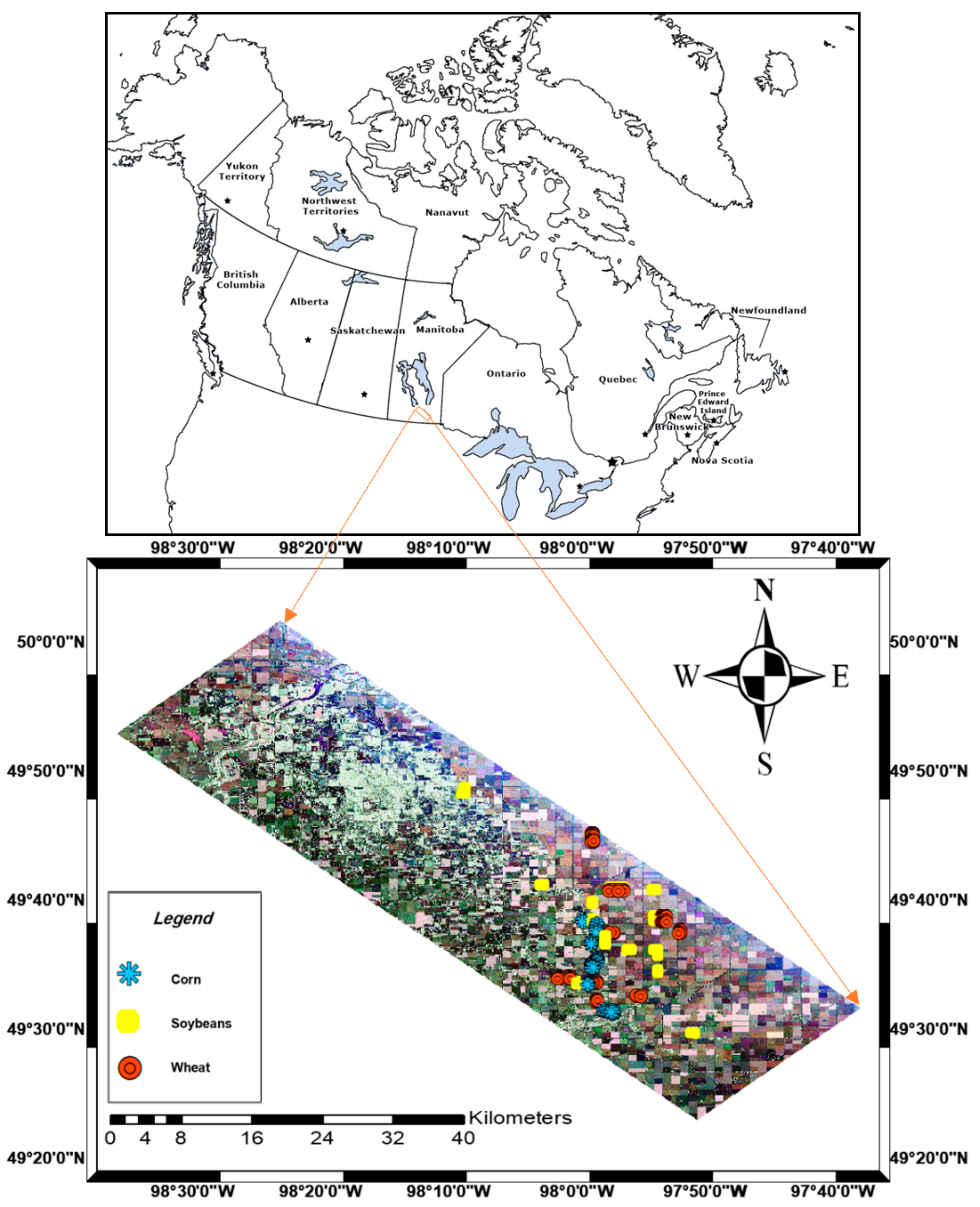
2.1. Study Site

This study uses data collected during the Soil Moisture Active Passive Experiment 2012 (SMAPVEX12). The SMAPVEX12 study area extends 12.8 km × 70 km and is located in a predominately annually cropped region of Manitoba, Canada (98°00′23″ W, 49°40′48″ N) (Figure 1). The soil textures vary significantly across this site, leading to large variances in surface soil moisture. Texture changes from heavy clay to fine loamy sands from east to west. This region of Canada has been the focus of extensive microwave soil moisture research given the importance of agriculture in this region of Canada and the variance in soil moisture within small geography [25,33,34]. In 2012, the crop breakdown within the SMAPVEX12 site included cereals (23.4% of the total crop acreage), canola (16.0%), corn (9.1%), soybeans (18.5%), and perennial cover (14.6%) [7].

2.2. UAVSAR Dataset

The airborne Uninhabited Aerial Vehicle Synthetic Aperture Radar (UAVSAR) is a mission-based, fully polarimetric L-band SAR sensor. UAVSAR data are available in several processing levels, including single-look complex (SLC), multi-look complex (MLC), ground-range detected (GRD), and compressed stoke matrix (DAT). The details of the UAVSAR system and its data are provided in Table 1. In this study, we considered the GRD product of flight line #31606 as this provided full coverage of all sampled agricultural fields with a 25° to 65° incidence angle [25]. The time-series of the UAVSAR dataset was acquired during the SMAPVEX12 project. The simultaneous UAVSAR flight with ground soil moisture sampling during SMAPVEX12 are listed in Table 2. The open source PolSARpro v.5 software developed by ESA (ESA, Paris, France) was used to generate the coherency matrix [T] and covariance matrix [C]. A boxcar filter with a 7 × 7 kernel size was applied for noise reduction. This site has minimal topographic variance and as such, no topographic correction was applied.

2.3. Ground Measurements

The SMAPVEX12 field campaign is fully described in [7], with an overview presented here. This campaign was executed over 6 weeks (6 June to 17 July 2012) with the intent to capture soil moisture conditions immediately following crop emergence to the period of peak biomass accumulation. Soil moisture measures were collected for 55 agricultural fields including 19 soybeans, 16 wheat, 8 corn, 7 canola, 4 pasture, and 1 forage field. Crews measured surface soil moisture (0–5.7 cm), coincident with the airborne flights, using handheld coaxial impedance-based dielectric reflectometry probes. In each of the 55 sample fields, soil moisture was measured at 16 sampling points, with three replicate measures at each point. These 16 points were located in two parallel rows designed to capture moisture conditions in an 800 m × 300 m area. In this study we considered the ground measured soil moisture data for soybeans, corn, and wheat fields. Each soil moisture measurement point in each field was used as an input to the retrieval algorithms. At these soil moisture sample points, the SAR extracted value was calculated as the average of 3 × 3 pixels around each point which covers the 18.2 m × 18.2 m region on the ground surface.
Surface roughness has a significant impact on the scattering characteristics (specular or diffuse) and as such, the magnitude of the incident microwave signal that scatters back to the sensor. It is important to consider the effects of soil roughness on the received total backscattered signal. Roughness changes due to tillage applications, and weathering effects. During SMAPVEX12, surface roughness parameters root means square height (RMS-H) and correlation length were measured using a 1 m length profilometer with 0.5 cm pin spacing at non-flight days as surface roughness parameters are less time-sensitive features. The RMS-H and correlation length equation demonstrated in Equations (1) and (2), respectively. In these equations, N refers to the number of pins in the profilometer, z i is height in location i from the ground in cm and z refers to the average of surface height in cm. ρ x is known as autocorrelation function and x refers to the degree of similarity between two distinct points in a specified distance. Two sites were dedicated to roughness measurement in each field. The roughness profilometers were located parallel to the UAVSAR look direction and digital images were acquired at a 118 cm distance from the profiler. If crop coverage was a hindrance to the profiler, the vegetation coverage was flattened before photo shooting. A 3 m profile was constructed by collecting three end-to-end profiles, replicated twice in each field. Profiles were collected at the beginning of the field campaign and re-collected if field crews noted significant changes in soil surface roughness in the course of the six week campaign.
S = i = 1 N z i 2 z 2 N 1 ,
ρ x = i = 1 N + 1 j z i z j + i 1 i = 1 N z i 2 .
The wheat biomass samples were gathered in a 0.5 m2 area. Soybeans and corn biomass samples were also gathered for ten plants in each field (each field consisted of two parallel rows with eight sample points in each row). This information provides valuable concepts over crop development stage impacts on SAR backscatter signal.
Valuable information was provided about the planting and harvest date of soybeans, wheat, and corn crops during SMAPVEX12 and also crop development at a different time interval during soil moisture data gathering by [35] (Table 3).

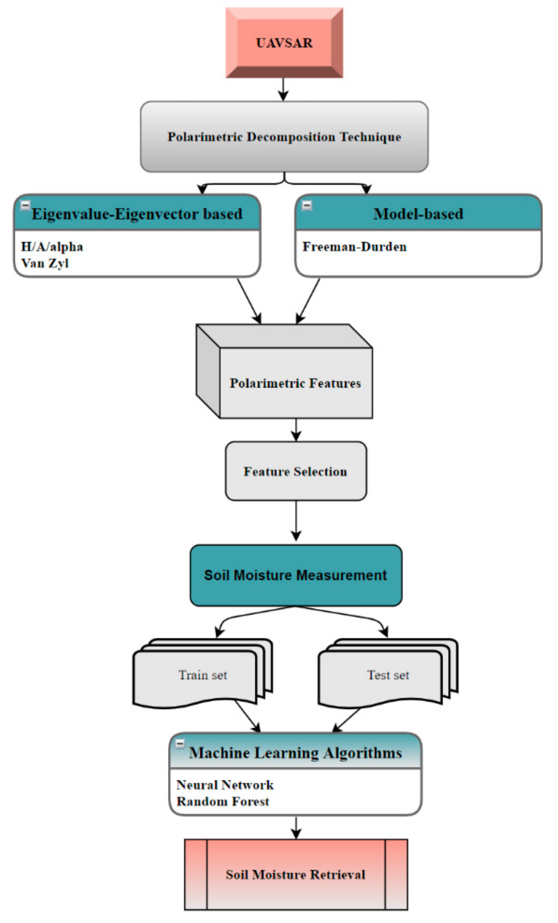
2.4. Polarimetric Decompositions

Quad polarimetric SAR sensors transmit alternate pulses of horizontal (H) and vertical (V) waveforms and record the intensity of both V and H polarized scattering and the phase difference between these two orthogonal polarizations [36]. A fully polarimetric system captures a complete picture of the scattering characteristics of a target and as such, is a powerful tool for target discrimination [19]. Polarimetric decomposition techniques can be applied to these complex data and may offer advantages in the retrieval of soil moisture estimates in the presence of vegetation cover. In this study, the potential of three decomposition models is assessed including the Freeman–Durden, Van Zyl, and H/A/α decompositions.
Model-based and eigenvalue-eigenvector decompositions, which are known as incoherent target decomposition approaches, are appropriate methods in the case of partially polarized target analysis to separate second-ordered coherency [T] and covariance [C] matrices. These matrices are derived from the scattering matrix (Equation (3)) and are used to extract polarimetric features.
S = S H H S H V S V H S V V .
Most natural features backscatter the SAR signals that are distributed which leads to backscatter of the collided signal to various directions. These targets are considered partially polarized. The distribution of scattering elements associated with these natural targets creates opportunities for single (surface) scattering events, dihedral (double bounce) events, and multiple (volume) scattering. The complex backscattering elements (intensity and phase) of the scattering matrix are demonstrated in Equation (3). S H H represents the radar signal transmitted in horizontal polarization and received in horizontal polarization. S H V and S V H represent signals transmitted in either H or V, but with the orthogonal polarization on receive. S V V quantifies the complex polarimetric signal transmitted and received in vertical polarization [37]. Four different descriptors, including Pauli and lexicographic vectors and covariance and coherency matrices, are extracted from the scattering matrix [S].
The coherency matrix [T] is constructed from the multiplication of the Pauli vector and its transpose conjugate [37]. On the other side, the covariance matrix is the result of the multiplication of the lexicographic vector and its transpose conjugate [38].

2.5. Freeman–-Durden Decomposition

The model-based three component Freeman–Durden decomposition extracts the volume, dihedral (double), and single bounce scattering submatrices from the second order covariance matrix [C] [24].
C 3 = C 3 v o l u m e + C 3 d o u b l e + C 3 s i n g l e ;
C 3 v o l u m e = f v 1 0 1 3 0 2 3 0 1 3 0 1 P v = 8 f v 3 ;
C 3 d o u b l e = f d α 2 0 α 0 0 0 α * 0 1 P d = f d 1 + α 2 ;
C 3 s i n g l e = f d β 2 0 α 0 0 0 α * 0 1 P s = f s 1 + β 2 .
The [C] matrix is composed of three [C] submatrices (Equations (5) to (7)) which refer to single bounce scattering, dihedral scattering, and volume scattering mechanisms of coherency matrix. The f v , f d , and f s represent the scattering amplitudes of volume, dihedral, and single bounce scattering component, respectively. P v , P d , and P s refer to volume, dihedral, and single bounce scattering powers, respectively. The α and β coefficients are the normalized difference of the Fresnel coefficients and the normalized difference of Bragg scattering between two HH and VV polarizations.
Freeman–Durden is an appropriate decomposition technique for vegetation-covered soils and has been evaluated for soil moisture retrieval [25,27,39].

2.6. Van Zyl Decomposition

The Van Zyl decomposition is an eigenvector-eigenvalue approach, which is known as a non-negative eigenvalue decomposition (NNED) [33]. Van Zyl et al., 2011 proposed this decomposition to evaluate the volume backscattering portion from vegetated regions [21]. In this approach, the covariance matrix is modified to remove negative eigenvalues. The radar cross section (RCS) is the ratio of the intensity of energy scattered from a target in the direction of the radar to the intensity of energy intercepted by a target. For natural distributed targets the RCS should have a non-negative value. Van Zyl et al. applied the Freeman–Durden and Yamaguchi decompositions to a SAR image of a heavily forested region in Germany. The outcome confirmed the existence of some pixels with negative power responses after the contribution of volume scattering was subtracted from the covariance matrix. The negative values do not have physical meaning with respect to these distributed targets. Van Zyl et al., 2011 proposed a modification to the covariance matrix (Equation (6)) to remove these negative values. The C m o d e l   is the covariance matrix predicted by other models and the C r e m a i n d e r   is a term representing a parameter not included in the C m o d e l covariance matrix. The eigenvalues should be non-negative in order for coefficient a in Equation (8) to have physical meaning.
C = a C m o d e l + C r e m a i n d e r .
The C r e m a i n d e r matrix is symmetric, as provided in Equation (9), to limit the values of the a coefficient. The eigenvalues of this matrix are described by Equation (10). The ξ ,   ς ,   ρ ,   and η parameters pertain to shape, statistical angular distribution, and size of the targets [32].
C r e m a i n d e r =   ξ 0 ρ 0 η 0 ρ * 0 ς a ξ a 0 ρ a 0 η a 0 ρ * a 0 ς a ,
λ 1 = 1 2 Y + X λ 2 = 1 2 Y X λ 1 = η a η a X = Y 2 4 ξ a ξ a ς a ς a + 4 ρ a ρ a 2 . Y = ξ + ς a ξ a a ς a

2.7. H/A/α Decomposition

Cloude and Pottier proposed an eigenvalue-eigenvector approach, known as H/A/α, as an incoherent target decomposition [20]. The coherency matrix, from which the H/A/α decomposition is extracted, is a positive Hermitian matrix that consists of three orthogonal eigenvectors and eigenvalues, equal to or greater than zero (Equation (11)). In this equation, [U] elements are considered as orthogonal eigenvectors, and λ parameters refer to real and non-negative eigenvalues. P i in Equation (12) expresses each scattering portion [19].
T = U 3 Σ U 3 1 ,
P i = λ i k = 1 3 λ k .
Three physical features can be extracted directly from this matrix, including entropy (H), alpha (α), and anisotropy (A) parameters that range from zero to one. The α parameter extracted from Equation (13) indicates the predominant scattering mechanisms. α equal or near zero is considered as surface scattering, α equal or near π 2 is indicative of dihedral scattering, and α near or equal π 4 is associated with volume scattering. The entropy parameter characterizes the degree of randomness of scattering within a target (Equation (14)). For targets with more predictable scattering, entropy approaches zero (H = 0). However, when scattering elements have a degree of random distribution, scattering is less predictable and entropy as a metric of randomness approaches one (H = 1). The third parameter can be extracted from the H/A/α parameter and is known as anisotropy (Equation (15)), which is interpretable when entropy is greater than 0.7. A defines the relationship and importance of the secondary and tertiary scattering components, λ 2 and λ 3 .
P i = λ i k = 1 3 λ k ,
H = i = 1 3 P i log 3 P i ,
A = λ 2 λ 3 λ 2 + λ 3               f o r     H > 0.7 .
Table 4 lists all the polarimetric features of the Freeman–Durden, Van Zyl, and H/A/α decompositions. The polarimetric and non-polarimetric features and soil parameters used in this study for the soil moisture modeling are also listed in Table 5.

2.8. Machine Learning Algorithms

Theoretical, empirical, and semi-empirical scattering models have been evaluated to retrieve soil moisture estimates from SAR data. Semi-empirical models include some elements of scattering theory but are simplified and require parameterization typically using field observational data. These parameterizations lead to limitations in terms of regions of validity with respect to SAR configurations (incidence angles, polarizations, and frequencies) and target conditions (soil moisture and surface roughness ranges). However, these models are much easier to invert and are thus more applicable to operational implementation. In addition to the complexity of theoretical scattering models, and the limitations in the applicability of semi-empirical models across wide-ranging conditions, these models do not easily capture the non-linearity between natural targets and SAR features. Machine learning approaches are more appropriate to model these non-linear relationships between output and input parameters [40,41]. In this study, because of the different ranges of feature values, a normalization process was implemented. As a result, the range of each feature was allocated between zero to one. Next, the dataset was randomly divided into training and testing subsets. Sample data were randomly selected for algorithm training (75% of the whole dataset) and independent validation (25% of the whole dataset). All accuracy metrics were calculated and demonstrated as results of this study on the unseen dataset (test set) for each algorithm.

2.8.1. Random Forest

Random forest (RF) is a robust machine learning algorithm that has been applied to both regression and classification problems and can address non-linear relationships between the target and input features [42,43]. As a supervised algorithm, RF requires sample training data. This algorithm creates the forest using a series of individual decision trees, each tree with a random subset of features [44]. Each tree accesses a random sub-dataset of training samples and predicts the target values. In the case of regression problems, each tree has a vote, and the prediction value is the average prediction of all decision trees. This algorithm can determine the relative importance of each input feature which is important in understanding the contribution of each feature to the RF output.
RF has been used as an ensemble learning approach to estimate soil moisture [45,46,47,48,49]. However, the use of polarimetric features as inputs to RF prediction of soil moisture is limited. This study investigates the ability of RF to estimate surface soil moisture from fully polarimetric SAR features. Due to the random operation of choosing features for each of the trees and to avoid overfitting issue, the algorithm was trained 50 times, then the average of all iterations was calculated on train and tested separately, and the results on the test set were considered as the absolute accuracy (Table 6). The train and test datasets were divided once and stayed fixed for all iterations. The RF was implemented using the python programming language using scikit-learn library.

2.8.2. Neural Network

Neural network (NN) regression has also been assessed for its ability to estimate soil moisture [29,50,51]. Neural networks are constructed from several neurons that make mathematical decisions to deal with complex issues. The simplest neural network has an input, hidden, and output layer. As the complexity of the problem increases, the complexity of the NN model also increases as more hidden layers are used. In this study, we use a feed-forward multi-layer perceptron (MLP) neural network [52]. We used the rectified linear units (ReLU) activation function. ReLU is an often-used activation function because it is less computationally expensive in comparison to other activation functions like Tanh and Sigmoid. The ReLU activation function is used as the non-linear function for hidden layers and as with other regression problems, a linear function was considered for the output layer.
To determine the best values for the weight parameters, the loss function provides the opportunity to specify the appropriate weights. There are different statistical parameters available in the regression context for loss value estimation such as root mean squared error (RMSE), mean absolute error (MAE), and mean bias error (MBE), which specify the goodness of weight parameters. Lower loss values indicate better weight parameters. In Equations (16) to (18) y i   refers to actual observation, y ^ i refers to model estimated values, and y ¯ i is the mean value of all y in the range 1 to N. N is the number of sample points. The R-squared, RMSE, MAE, and MBE parameters are used as metrics of model accuracy (Equations (16) to (19)).
R M S E = 1 N i = 1 N y i y ^ i 2 ,
M A E = 1 N i = 1 N y i y ^ i ,
R 2 = 1 1 N i = 1 N y i y ^ i 2 1 N i = 1 N y i y ¯ i 2 ,
M B E = 1 N i = 1 N y ^ i y i .
Figure 2 demonstrates the flowchart of this study as explained earlier.
In this study, all accuracy metrics including R-squared, RMSE, and MAE parameters were calculated and demonstrated in the results section on the test set subcategory to evaluate the performance of the trained algorithm on an unseen dataset. All accuracy parameters evaluated in Python Programming Language using scikit-learn library.

2.9. Feature Selection

Feature selection helps to order features in terms of their importance in algorithm performance and with respect to their performance in predictions [53,54]. Feature selection helps to prune inputs to prevent overfitting and reduces training time. In some cases, the presence of irrelevant features can negatively impact results and reduce the final accuracy [55]. In real world regression problems like soil moisture retrieval, a non-linear relationship exists between features and target. Also, in most cases, all features have non-normal distribution and lie in different ranges. To deal with these problems, all datasets were normalized before preprocessing to bring all feature values to the specified range. There are different manual and automatic methods for feature selection including trial and error, backward feature selection, and forward feature selection methods, with three selected for evaluation in this study.

2.9.1. Trial and Error

In this study, the Pearson correlation matrix, in this study known as correlation matrix, is used to document the correlation between soil moisture and each polarimetric feature. This graphic is also a convenient approach to tabulate the correlation between features. The high correlation coefficient is indicative of the redundancy of some features [56]. To assess whether highly correlated features lead to R-squared reduction or not which is a debatable topic, the performance of the algorithm was tested by adding remaining features that are highly correlated to the main features (R-squared > |0.5|).
As an initial step, polarimetric features were arranged based on their individual correlation (linear correlation) with soil moisture. Next, the features with the highest correlation (labeled here as main features) were used individually in the soil moisture algorithms and assessed for accuracy. To determine if the value is added by including additional remaining polarimetric features, the correlation between main and remaining features were calculated. Correlated features can decrease estimation accuracy and typically the most relevant features for target estimation are not highly correlated. To test this hypothesis, a ± 0.5 Pearson correlation coefficient (R) value threshold was set. Feature sets are divided into two categories. Category one contains remaining features with a correlation to main features of less or equal to |0.5| and category two with correlations more than |0.5|. As the first step, features in category one were arranged based on lower to higher correlation value with the ‘main’ feature. The features were added to the algorithm based on their arrangement. After each feature entrance, the accuracy metric (R-squared) was assessed to evaluate the performance of each feature on accuracy modification. The remaining features are retained only if R-squared accuracies of soil moisture estimation did not change or accuracies increased. After testing the features in category one, all the above-mentioned steps were repeated on highly correlated features (category two). In some cases, the addition of these highly correlated features not only does not reduce accuracies but also improves soil moisture estimates. Given these findings, the correlated features which improved accuracies are retained. The list of selected features is provided in Table 5.

2.9.2. Backward Feature Selection (BFS)

BFS is a wrapper feature selection technique that uses a grid search procedure for irrelevant feature elimination [57]. In this technique, all of the features were used as initial inputs to the algorithm. Then the process of removing the least relevant features was initiated and the performance of the algorithm was evaluated in each iteration. The element which had the least positive effect on algorithm performance was deleted. The metric for performance evaluation of the model was a p-value greater than 0.05 which means that the features that have p-values greater than 0.05 are deleted from the feature list. These steps were repeated until a level of stability was reached, such that the R-squared value did not change significantly by removing the features.

2.9.3. Forward Feature Selection (FFS)

FFS is another wrapper feature selection technique that is initiated with an empty set of features [58]. Features were first normalized to values from zero to one. Then the correlation between features was evaluated and features with a correlation (R-value) that exceeds |0.5| were removed from the input list. All remaining elements were evaluated separately. In each iteration, the feature that provided the best accuracy was selected and retained. In each subsequent iteration, the remaining features were added to the last version to find the next best feature. This procedure continued until all the features were assessed. One of the negative points of this algorithm relates to this fact that by adding a feature to the algorithm, it would not be removed from the algorithm.

3. Results

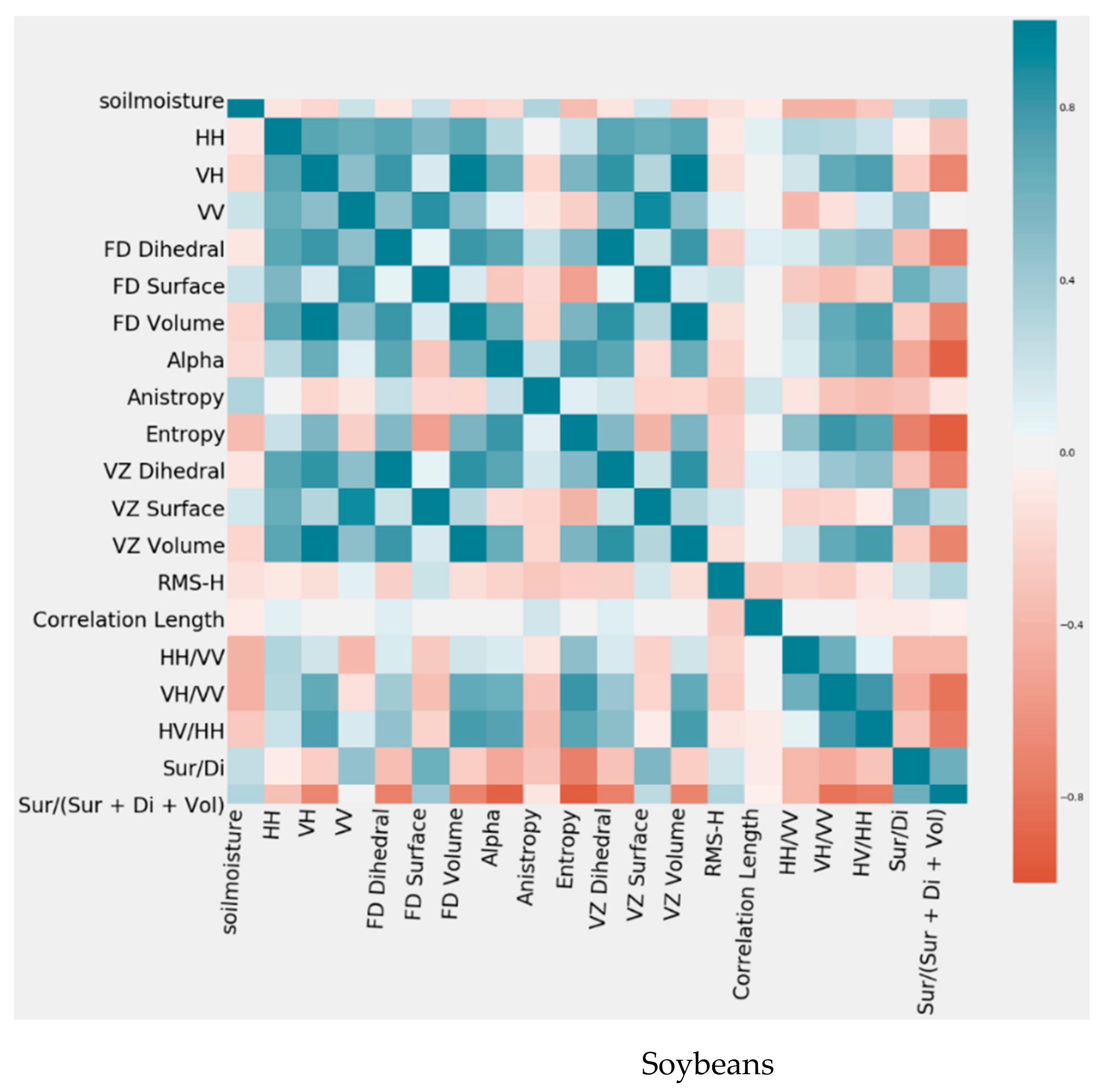
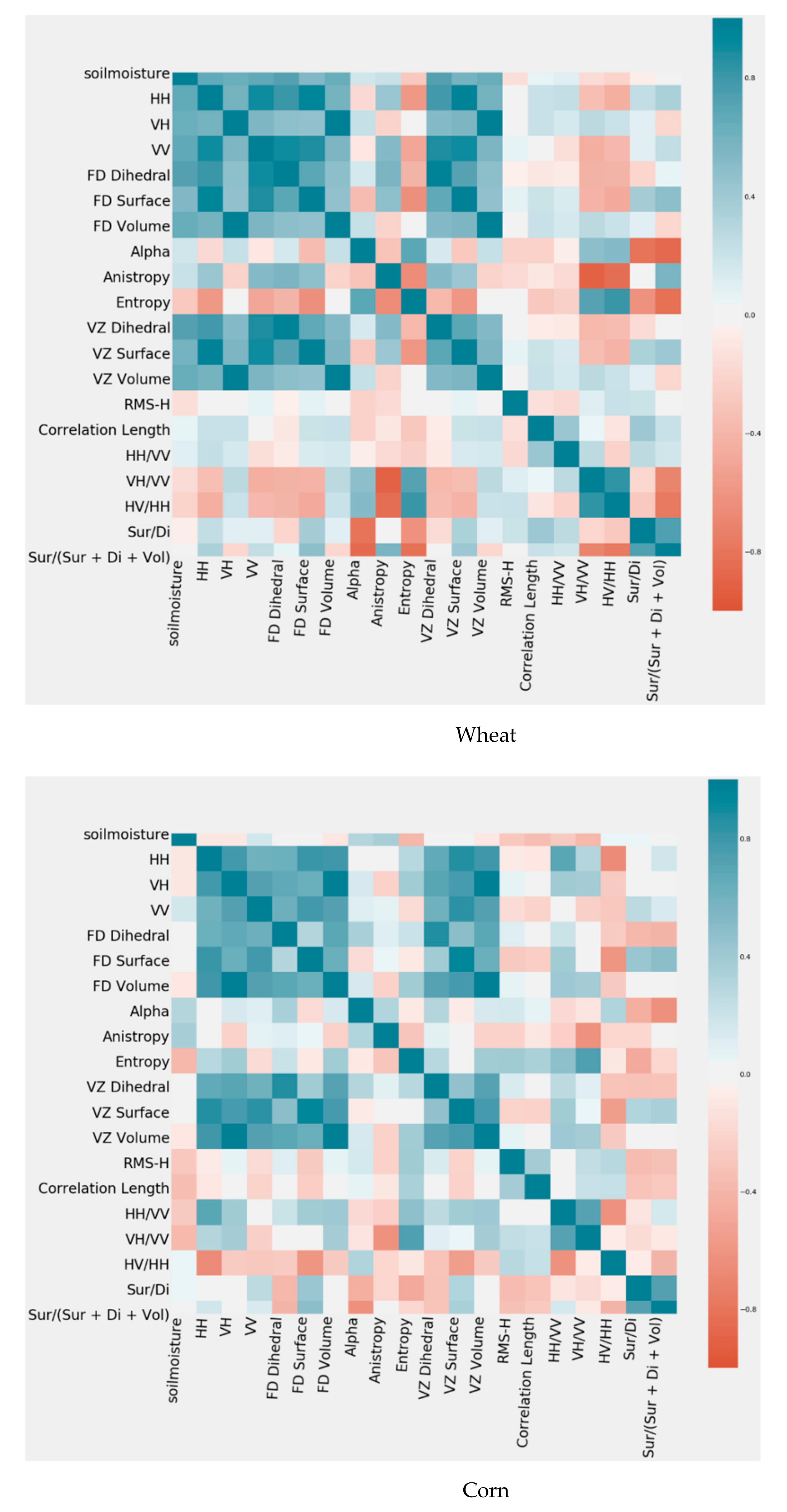
3.1. Feature Selection

Correlation matrixes were generated for each individual crop to document the correlation between measured soil moisture and each feature, as well as among features. These correlation matrixes for soybeans, wheat, and corn are provided in Figure 3.
A cross-comparison of results from the three feature selection approaches is documented in Table 6. Features including the roughness parameters (RMS-H and correlation length) were selected regardless of which selection method was applied. The roughness parameters highly affected SAR backscattered signals which led to over and underestimation of soil moisture retrieval. It is therefore logical that the availability of surface roughness information helps soil moisture retrieval with higher accuracy. In some cases, the HH backscatter parameter also showed good performance for soil moisture retrieval which proves the sensitivity of HH polarization to moisture content. In most cases, anisotropy parameter was one of the most important parameters in different algorithms. As expressed by Cloude et al., 2000 [59] and Hajnesk et al., 2002 [60] anisotropy parameter is sensitive to soil surface roughness. This suggests that these parameters are likely to be important contributors to soil moisture retrieval. Other features, including volume scattering freeman, dihedral scattering van zyl, H V H H and surface   scattering surface   +   dihedral   +   volume are selected only by some of the feature selection methods. These features may contribute to the modeling of moisture but are likely to be less important.

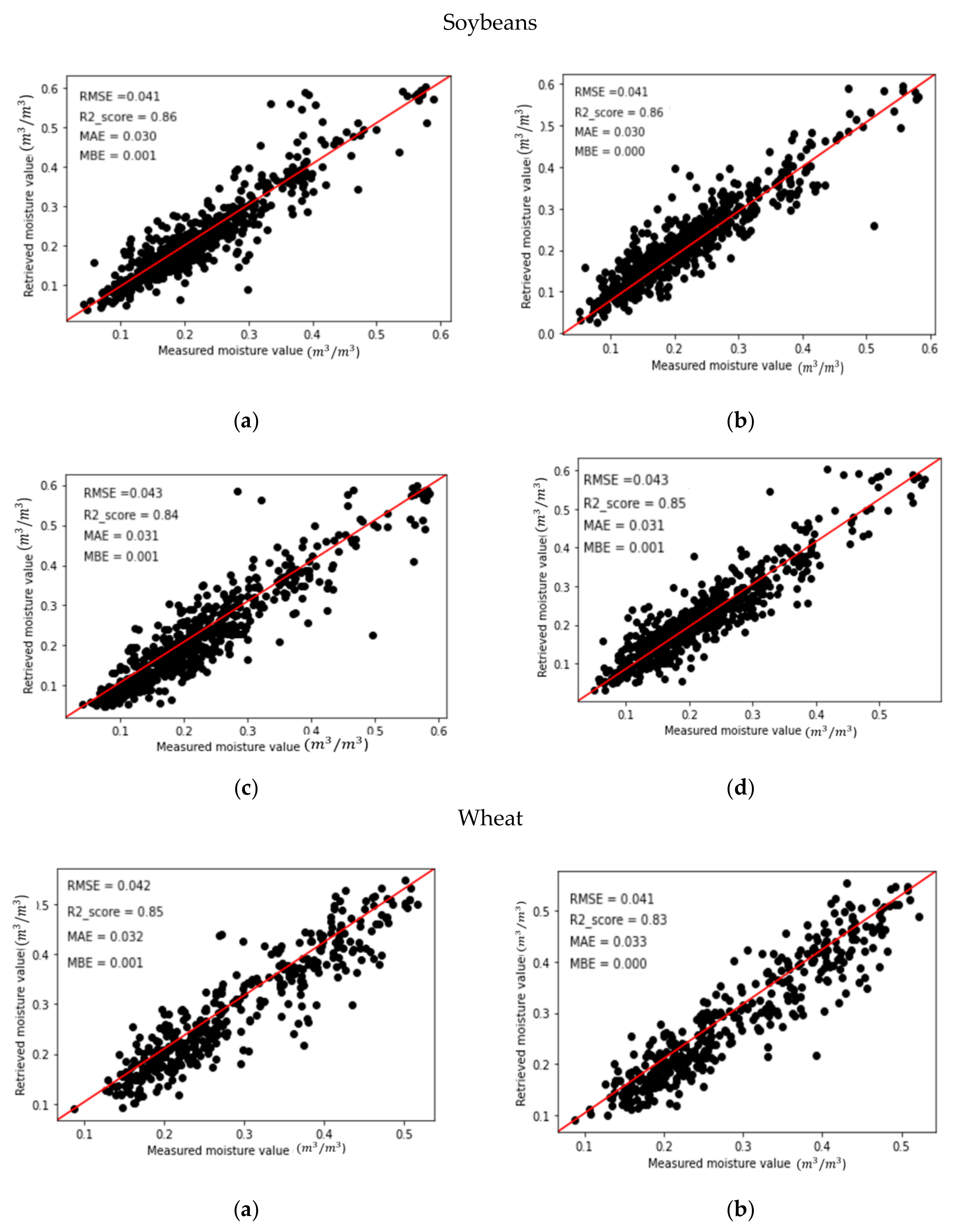
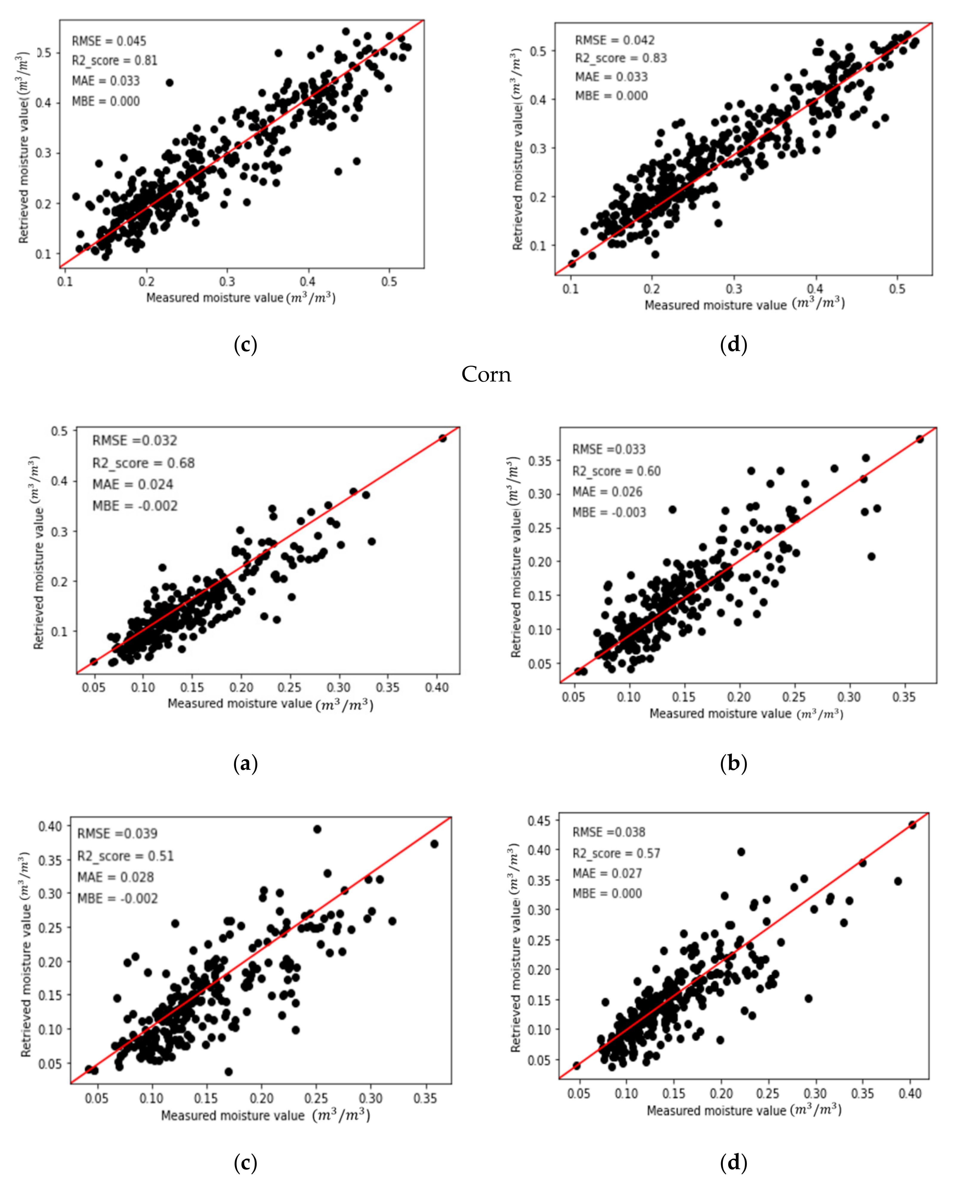
3.2. Soil Moisture Estimation Using a Random Forest (RF) Algorithm

The accuracy of soil moisture retrieval, using features selected by trial and error, is similar to accuracies when all features are used in an RF algorithm. As such, from this analysis, it is reasonable to conclude that a limited number of features (in this case less than half) can deliver accurate soil moisture estimates. Some features, specifically the surface roughness parameters (RMS-H and Correlation Length), are selected for all RF runs. Some features like alpha and anisotropy are chosen from most runs. The feature importance option in RF models provides this opportunity to rank the features as very convenient and efficient. From this option, the authors found out and acknowledged that selected features (features with higher importance) have higher importance for soil moisture retrieval. The best results are reported for soybeans. For this crop, features selected using trial and error as inputs to the RF delivered a high correlation of determination of R2 = 0.86. The poorest results were found when the FFS feature selection was applied to estimate soil moisture for corn fields (R2 = 0.51). (More accurate soil moisture estimates were reported for soybean fields compared to wheat and corn. The canopy of soybean crops was more open and soybeans accumulated less above-ground biomass. For corn and wheat crops, SAR signals interacted more with less large canopies, and even at L-band, less direct soil scattering contributions occurred.
Trial and error feature reduction procedure delivered results comparable to soil moisture retrieval outcomes when all features were input. In the final step of trial and error some highly correlated features were retained, and these remaining features although highly correlated with main features, appeared to be important in soil moisture retrieval. The features selected by the BFS delivered the second most accurate estimates, with the FFS selected features the least accurate. The FFS feature reduction method, coupled with the RF algorithm, produced the lowest soil moisture accuracies for all crop types, and this may be due to the fact that FFS selects the fewest input features. All the accuracy results in Table 7 are acquired from the unseen dataset. Soil moisture retrieval results over test dataset are given in Figure 4.
The red line is known as the line of best fit. This line in each scatter plot best expresses the relationship between measured and estimated moisture value. The closer sample points to line of best fit leads to higher correlation values between measured and retrieved soil moisture increases. Like any real-world issue, it’s a very usual phenomenon that predicted values for some sample point could be different from ground truth values. SAR signal is sensitive to different parameters in addition to soil moisture including vegetation effects and also surface roughness parameters. These parameters lead to biases when it comes to the sample points located outside the line of best fit.

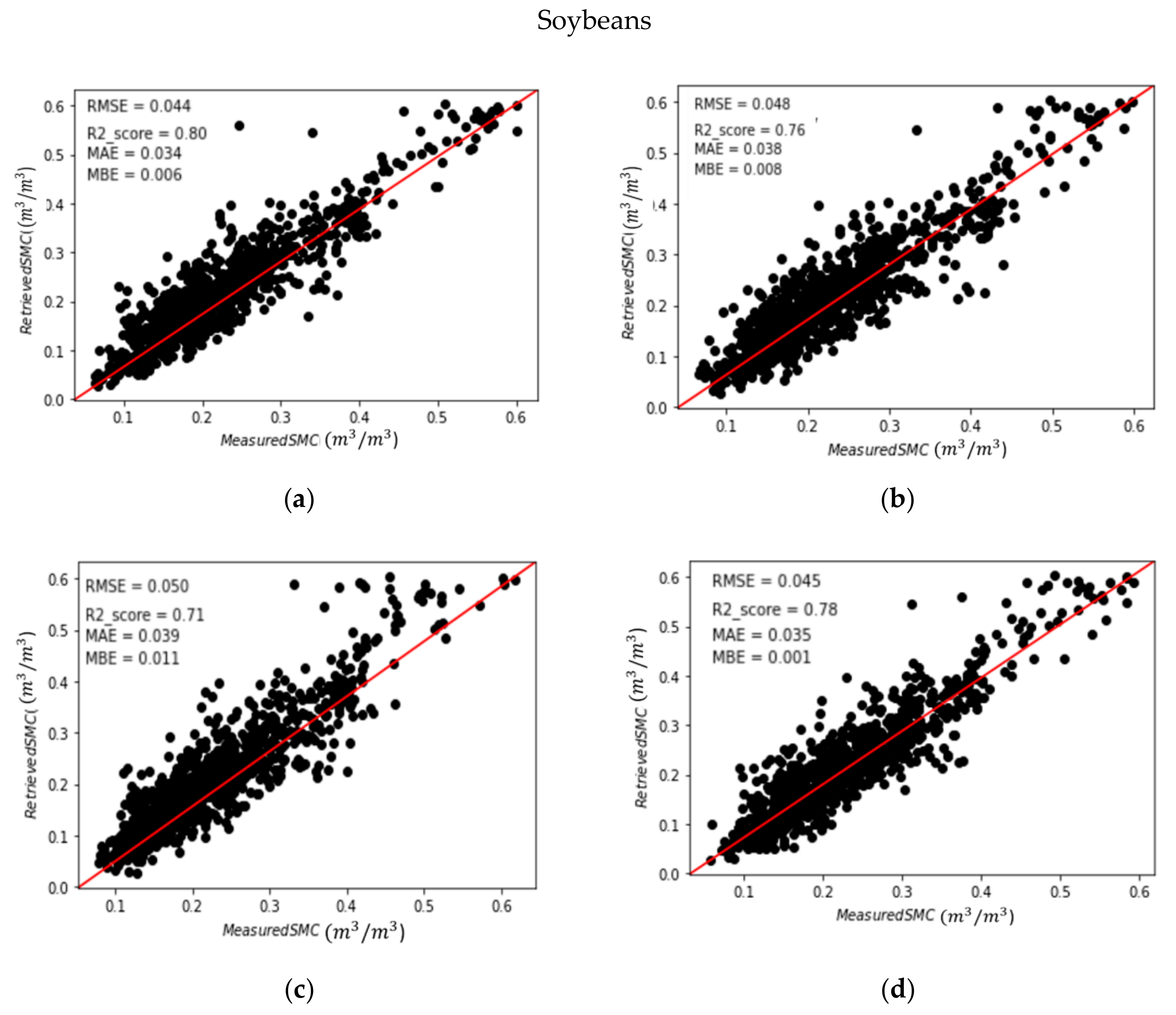
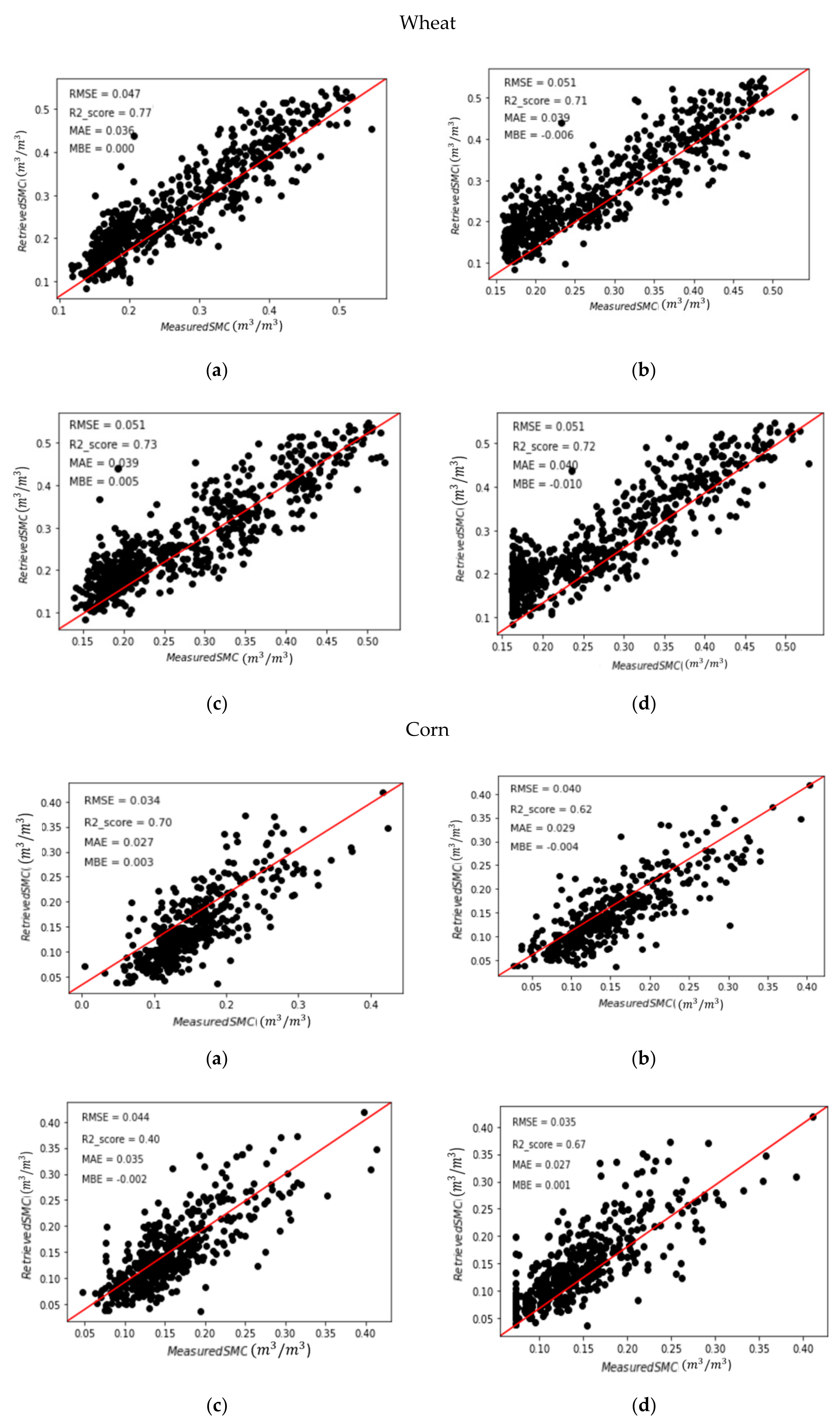
3.3. Soil Moisture Estimation Using a Neural Network Algorithm

As with the RF analysis, the NN algorithm was tested for soil moisture retrieval using all available features as well as features selected by trial and error, BFS, and FFS methods. Soil moisture retrieval results for the validation dataset for each feature selection method and crop type are given in Figure 5 and Table 8.
The best results are obtained using all the extracted features. As with the RF runs, the most accurate estimates of soil moisture using an NN are for soybean fields with R2 = 0.80 (all extracted features used as inputs). The highest errors are reported for corn using FFS selected features R2 = 0.40. The poorer performance for corn fields is not unexpected given the large biomass associated with this crop canopy. At peak biomass, corn fields in the SMAPVEX12 study site had approximately four times the fresh biomass relative to soybean crops (approximately 4000 gm−2 for corn compared to 1000 gm−2 for soybean) [35] with the height of the corn canopy averaging 2–2.5 m at peak growth [61]. The size of this corn canopy would impede even L-band wavelengths (here 23.8 cm) from reaching the soil unimpeded by volume scattering from the crop leaves and stalks. Soybean canopies are not only lower in biomass and height, but have wider row spacing than crops like wheat. In this region of Manitoba, soybean row spacing varies but the median spacing between rows is relatively high (approximately 64 cm). This lower canopy and wider row spacing offer ample opportunity for the penetration of L-band waves and direct interaction with the soil. The BFS approach selected about half of the available features, with the best performance for soil moisture retrieval for soybean, wheat, and corn fields. Outcomes in Table 8 were acquired on the test dataset.

3.4. Comparison between RF and NN Algorithms

When the results of the RF and NN algorithms were compared using the same selected features, random forest estimates soil moisture to a higher accuracy regardless of crop type.
Several parameters have direct impacts on backscattered SAR signals toward the sensor including the crop height and biomass [24]. At early crop growth stages, most of the backscatter is related to soil surface impacts. Moving forward to the middle of the growing season, the soil surface impacts on the backscattered signal is decreased and it reaches its lowest amount at the pick of the crop growth stage. During the SMAPVEX12 campaign, data were collected from crop emergence (17 June) to fully developed crop growth stages (17 July). Therefore, the vegetation impacts on soil moisture estimation modeling were significant. However, using the polarimetric decomposition parameters, the soil moisture estimation accuracies were at the promising RMSE range of 0.03–0.05 m3 m−3 for both RF and NN algorithms and all the crop types.

4. Discussion

This study investigates the potential of L-Band Synthetic Aperture Radar (SAR) polarimetric features for soil moisture retrieval under three crop canopies (corn, soybeans, and wheat). Three feature selection approaches are assessed including trial and error, BFS, and FFS. The polarimetric features evaluated are derived from the model-based Freeman–Durden decomposition and the Eigenvalue-Eigenvector based H/A/α and Van Zyl decompositions. Other SAR inputs include backscatter intensities (HH, VV, and HV polarizations), polarization ratios, and roughness parameters. Selected features are used as input into both a random forest and the multi-layer perceptron neural network algorithm with estimated soil moisture validated against field-measured moisture. The research uses airborne UAVSAR data and field data collected in Manitoba (Canada) during the Soil Moisture Active Passive Validation Experiment 2012 (SMAPVEX12).
Considering other studies, Özerdem et al., 2017 [27] used the backscattering coefficients, H/A/α and Freeman–Durden polarimetric features extracted from the C-band quad polarimetric Radarsat-2 data to retrieve soil moisture over agricultural regions. They used the Generalized Regression Neural Network as their soil moisture estimation algorithm. They divided their dataset into bare soil, low vegetation cover, and high vegetation cover and derived R = 0.92, R = 0.80, R = 0.74 between the measured and estimated soil moisture for these three vegetation cover ranges, respectively. Özerdem et al., 2017 stated that the lack of surface roughness data was one of the main restrictions. Also, the crop type is not determined in this study. In another case, Wang et al., 2016 [24] confined the potential of model-based Cloude–Pottier to surface scattering mechanism. They retrieved soil moisture with RMSE = 0.06 to 0.12 m3 m−3 just on pixels with dominant surface scattering mechanism. The proposed method restricted the proposed algorithm’s capability for soil moisture retrieval over regions with dominant volume and dihedral scattering mechanisms. In other research, Wang et al., 2017 [25] checked the potential of three polarimetric model-based decompositions (Freeman–Durden, Hajnesk, and An) for soil moisture retrieval. They removed the volume scattering component to investigate the potential of surface and dihedral scattering mechanisms over corn, canola, soybeans, and wheat vegetation covered fields. However, they neglected the potential of volume scattering component on soil moisture retrieval over the agricultural region. Hajdu et al., 2018 [30] used C-band Sentinel-1 data and the random forest algorithm for soil moisture estimation over agricultural fields. They used a backscattered signal (VV polarization, vegetation index, and terrain attributes (slope, aspect, roughness, and wetness index)) for soil moisture retrieval. Similar to what we demonstrated in this study, their results showed that random forest was able to learn the non-linear relationship between ground-based and remotely-sensed parameters and derived R2 = 0.86 between the measured and estimated soil moisture. Hajdu et al. used a dual-polarized dataset which records the limited complexity of the targets in comparison to the Polarimetric SAR dataset. Millard et al., 2018 [62] used Polarimetric Radarsat-2, MODIS, and Lidar data for soil moisture prediction in presence of dynamic surface and vegetation phenomena. The vegetation information was derived from a multi-date MODIS dataset. They applied empirical CART and random forest regression models for soil moisture retrieval to determine the relationship between SAR derived variables, Lidar-derived dynamic surface roughness, vegetation features at the vegetation-covered region with ground measured soil moisture values. Using Lidar-derived dynamic parameters is one of the attractive points of Millard’s study which provides the opportunity to evaluate the effect of surface roughness without ground-measured values.
In comparison to some studies like what was proposed by Hadju et al., 2018 and Millard et al., 2018, which used multi-source information, our results prove that the potential of polarimetric SAR extracted features provide comparable results for highly accurate soil moisture retrieval using only UAVSAR dataset. In comparison to some studies which retrieved soil moisture using dual-polarized information, a fully polarimetric UAVSAR sensor can record more information. The results obtained from some studies (like [27,30]) confirm the fact that more and various feature extraction could not be a solution for soil moisture retrieval with better accuracy. One of the main results in this study shows that in some cases the same accuracy could be obtained using a lower number of features.
In this research, the authors also utilized the potential of volume and dihedral scattering like surface scattering and did not refuse part of this information for soil moisture retrieval over vegetation coverage. In our study, it was also proven that the roughness parameters have significant impacts on soil moisture retrieval accuracy. A brief description of the above-mentioned studies is listed in Table 9. The algorithms were tested over soybeans, wheat, and corn crops separately to determine the potential of the same NN-MLP and RF algorithms over a specific feature set for each field. The results obtained from these studies confirm the fact that more and various feature extraction could not be a solution for soil moisture retrieval with the highest accuracy. One of the main results in this study shows that in some cases the same accuracy could be obtained using a lower number of features and some features like roughness parameters, HH backscatter intensity, and anisotropy features were most important for soil moisture retrieval over this agricultural landscape. The final results show comparable results with similar studies as demonstrated in Table 9.
The algorithms were tested over soybeans, wheat, and corn crops separately to determine the potential of the same NN-MLP and RF algorithms over a specific feature set for each field. The results obtained from these studies confirm the fact that more and various feature extraction could not be a solution for soil moisture retrieval with the highest accuracy. One of the main results in this study shows that in some cases the same accuracy could be obtained using a lower number of features and some features like roughness parameters, HH backscatter intensity, and anisotropy features were most important for soil moisture retrieval over this agricultural landscape. The final results show comparable results with similar studies as demonstrated in Table 9.

5. Conclusions

According to this research, the random forest algorithm provides higher accuracies for soil moisture estimation when compared to the neural network when using identical features. The better performance of the RF is observed for all three crop types and holds regardless of the feature selection methods used (trial and error, BFS, or FFS). The best results are achieved for lower biomass soybean fields using the RF, with statistical performance metrics of the coefficient of determination R2 = 0.86, root mean square error (RMSE) = 0.041 m3 m−3 and mean average error (MAE) = 0.030 m3 m−3. The least accurate results are reported for corn canopies using a NN algorithm and the FFS feature selection approach (R2 = 0.40, RMSE = 0.044 m3 m−3 and MAE = 0.035 m3 m−3). This study demonstrated that the accuracy of soil moisture estimation does not depend exclusively on the number of features selected for input to retrieval algorithms. That means in some cases, relatively similar results were obtained using fewer features.
Until now, no ground soil moisture measurement project had measured surface roughness for all sample points. Due to the considerable effect of surface roughness for high accuracy soil moisture retrieval, the roughness parameters could be provided using some factors like the land cover, land usage, or very high-resolution bare earth DEM in future studies.

Author Contributions

Z.A. and M.H. (Mahdi Hasanlou) did preprocesses and prepared datasets. Z.A., M.H. (Mahdi Hasanlou) and M.H. (Mehdi Hosseini) designed modeling concepts and implemented the soil moisture process. Z.A., M.H. (Mahdi Hasanlou), M.H. (Mehdi Hosseini) and H.M. wrote and checked the manuscript. All authors have read and agreed to the published version of the manuscript.

Funding

This research received no external funding.

Institutional Review Board Statement

Not applicable.

Informed Consent Statement

Not applicable.

Data Availability Statement

Not applicable.

Acknowledgments

The Authors would like to thank all crews of the SMAPVEX12 project for collecting this valuable dataset. The authors also thank the National Aeronautics and Space Administration (NASA) for providing the Quad Polarimetric UAVSAR datasets and the Canadian and USA funding support agencies for the SMAPVEX12 ground sampling project.

Conflicts of Interest

The authors declare no conflict of interest.

References

  1. Johnston, B.R.; Hiwasaki, L.; Klaver, I.J.; Ramos Castillo, A.; Strang, V. Water, Cultural Diversity, and Global Environmental Change: Emerging Trends, Sustainable Futures? Springer Science & Business Media: Berlin/Heidelberg, Germany, 2011. [Google Scholar]
  2. Schoonover, J.E.; Crim, J.F. An introduction to soil concepts and the role of soils in watershed management. J. Contemp. Water Res. Educ. 2015, 154, 21–47. [Google Scholar] [CrossRef]
  3. Cosh, M.H.; Jackson, T.J.; Bindlish, R.; Prueger, J.H. Watershed scale temporal and spatial stability of soil moisture and its role in validating satellite estimates. Remote Sens. Environ. 2004, 92, 427–435. [Google Scholar] [CrossRef]
  4. Jackson, T.J.; Bindlish, R.; Gasiewski, A.J.; Stankov, B.; Klein, M.; Njoku, E.G.; Bosch, D.; Coleman, T.L.; Laymon, C.A.; Starks, P. Polarimetric scanning radiometer C-and X-band microwave observations during SMEX03. IEEE Trans. Geosci. Remote Sens. 2005, 43, 2418–2430. [Google Scholar] [CrossRef]
  5. Cosh, M.H.; Jackson, T.J.; Starcks, P.; Heathman, G. Temporal stability of surface soil moisture in the Little Washita River watershed and its applications in satellite soil moisture product validation. J. Hydrol. 2006, 323, 168–177. [Google Scholar] [CrossRef]
  6. Bhuiyan, H.A.; McNairn, H.; Powers, J.; Friesen, M.; Pacheco, A.; Jackson, T.J.; Cosh, M.H.; Colloander, A.; Berg, A.; Rowlandson, T.; et al. Assessing SMAP soil moisture scaling and retrieval in the Carman (Canada) study site. Vadose Zone J. 2018, 17, 1–14. [Google Scholar] [CrossRef] [Green Version]
  7. McNairn, H.; Jackson, T.J.; Wiseman, G.; Belair, S.; Berg, A.; Bullock, P.; Colloander, A.; Cosh, M.H.; Kim, S.; Moghaddam, M.; et al. The soil moisture active passive validation experiment 2012 (SMAPVEX12): Prelaunch calibration and validation of the SMAP soil moisture algorithms. IEEE Trans. Geosci. Remote Sens. 2014, 53, 2784–2801. [Google Scholar] [CrossRef]
  8. Malik, M.S.; Shukla, J. Estimation of Soilmoisture by Remote Sensing and Field Methods: A Review. Int. J. Remote Sens. Geosci. 2014. [Google Scholar] [CrossRef] [Green Version]
  9. Ma, C.; Li, X.; McCabe, M.F. Retrieval of High-Resolution Soil Moisture through Combination of Sentinel-1 and Sentinel-2 Data. Remote Sens. 2020, 12, 2303. [Google Scholar] [CrossRef]
  10. Baghdadi, N.; Choker, M.; Zribi, M.; El Hajj, M.; Paloscia, S.; Verhoest, N.E.C.; Lievens, H.; Baup, F.; Mattia, F. A new empirical model for radar scattering from bare soil surfaces. Remote Sens. 2016, 8, 920. [Google Scholar] [CrossRef] [Green Version]
  11. Zribi, M.; Dechambre, M. A new empirical model to retrieve soil moisture and roughness from C-band radar data. Remote Sens. Environ. 2003, 84, 42–52. [Google Scholar] [CrossRef]
  12. Thoma, D.; Moran, M.S.; Bryant, R.; Rahman, M.; Holfield-Collons, C.D.; Skirvin, S.; Sano, E.E.; Slocum, K. Comparison of four models to determine surface soil moisture from C-band radar imagery in a sparsely vegetated semiarid landscape. Water Resour. Res. 2006, 42. [Google Scholar] [CrossRef] [Green Version]
  13. Altese, E.; Bolognani, O.; Mancini, M.; Torch, P.A. Retrieving soil moisture over bare soil from ERS 1 synthetic aperture radar data: Sensitivity analysis based on a theoretical surface scattering model and field data. Water Resour. Res. 1996, 32, 653–661. [Google Scholar] [CrossRef]
  14. Oh, Y. Quantitative retrieval of soil moisture content and surface roughness from multipolarized radar observations of bare soil surfaces. IEEE Trans. Geosci. Remote Sens. 2004, 42, 596–601. [Google Scholar] [CrossRef]
  15. Baghdadi, N.; Zribi, M. Evaluation of radar backscatter models IEM, OH and Dubois using experimental observations. Int. J. Remote Sens. 2006, 27, 3831–3852. [Google Scholar] [CrossRef]
  16. Hosseini, M.; Saradjian, M. Soil moisture estimation based on integration of optical and SAR images. Can. J. Remote Sens. 2011, 37, 112–121. [Google Scholar] [CrossRef]
  17. Gherboudj, I.; Magagi, R.; Berg, A.; Toth, B. Soil moisture retrieval over agricultural fields from multi-polarized and multi-angular RADARSAT-2 SAR data. Remote Sens. Environ. 2011, 115, 33–43. [Google Scholar] [CrossRef]
  18. Ulaby, F.T.; Aslam, A.; Dobson, M.C. Effects of vegetation cover on the radar sensitivity to soil moisture. IEEE Trans. Geosci. Remote Sens. 1982, 476–481. [Google Scholar] [CrossRef]
  19. Cloude, S.R.; Pottier, E. A review of target decomposition theorems in radar polarimetry. IEEE Trans. Geosci. Remote Sens. 1996, 34, 498–518. [Google Scholar] [CrossRef]
  20. Cloude, S.R.; Pottier, E. An entropy based classification scheme for land applications of polarimetric SAR. IEEE Trans. Geosci. Remote Sens. 1997, 35, 68–78. [Google Scholar] [CrossRef]
  21. Ustuner, M.; Balik Sanli, F. Polarimetric target decompositions and light gradient boosting machine for crop classification: A comparative evaluation. ISPRS Int. J. Geo Inf. 2019, 8, 97. [Google Scholar] [CrossRef] [Green Version]
  22. Jagdhuber, T. Soil Parameter Retrieval under Vegetation Cover Using SAR Polarimetry. Ph.D. Thesis, Universitätsbibliothek Potsdam, Potsdam, Germany, 2012. [Google Scholar]
  23. Lee, J.-S.; Pottier, E. Polarimetric Radar Imaging: From Basics to Applications; CRC press: Boca Raton, FL, USA, 2017. [Google Scholar]
  24. Wang, H.; Magagi, R.; Goita, K.; Jagdhuber, T.; Hajnesk, I. Evaluation of simplified polarimetric decomposition for soil moisture retrieval over vegetated agricultural fields. Remote Sens. 2016, 8, 142. [Google Scholar] [CrossRef] [Green Version]
  25. Wang, H.; Magagi, R.; Goita, K. Comparison of different polarimetric decompositions for soil moisture retrieval over vegetation covered agricultural area. Remote Sens. Environ. 2017, 199, 120–136. [Google Scholar] [CrossRef]
  26. Hajnsek, I.; Jagdhuber, T.; Schon, H.; Papathanassiou, K.P. Potential of estimating soil moisture under vegetation cover by means of PolSAR. IEEE Trans. Geosci. Remote Sens. 2009, 47, 442–454. [Google Scholar] [CrossRef] [Green Version]
  27. Özerdem, M.S.; Acar, E.; Ekinci, R. Soil moisture estimation over vegetated agricultural areas: Tigris Basin, Turkey from Radarsat-2 data by polarimetric decomposition models and a generalized regression neural network. Remote Sens. 2017, 9, 395. [Google Scholar] [CrossRef] [Green Version]
  28. Lary, D.J.; Alavi, A.H.; Gandomi, A.H.; Walker, A.L. Machine learning in geosciences and remote sensing. Geosci. Front. 2015, 30, 1e9. [Google Scholar] [CrossRef] [Green Version]
  29. El Hajj, M.; Baghdadi, N.; Zribi, M.; Bazzi, H. Synergic use of Sentinel-1 and Sentinel-2 images for operational soil moisture mapping at high spatial resolution over agricultural areas. Remote Sens. 2017, 9, 1292. [Google Scholar] [CrossRef] [Green Version]
  30. Hajdu, I.; Yule, I.; Dehghan-Shear, M.H. Modelling of near-surface soil moisture using machine learning and multi-temporal sentinel 1 images in New Zealand. In Proceedings of the IGARSS 2018–2018 IEEE International Geoscience and Remote Sensing Symposium, Valencia, Spain, 22–27 July 2018. [Google Scholar]
  31. Freeman, A.; Durden, S.L. A three-component scattering model for polarimetric SAR data. IEEE Trans. Geosci. Remote Sens. 1998, 36, 963–973. [Google Scholar] [CrossRef] [Green Version]
  32. Van Zyl, J.J.; Arii, M.; Kim, Y. Model-based decomposition of polarimetric SAR covariance matrices constrained for nonnegative eigenvalues. IEEE Trans. Geosci. Remote Sens. 2011, 49, 3452–3459. [Google Scholar] [CrossRef]
  33. Hosseini, M.; McNairn, H. Using multi-polarization C-and L-band synthetic aperture radar to estimate biomass and soil moisture of wheat fields. Int. J. Appl. Earth Obs. Geoinf. 2017, 58, 50–64. [Google Scholar] [CrossRef]
  34. Wang, H.; Magagi, R.; Goita, K.; Jagdhuber, T. Refining a polarimetric decomposition of multi-angular UAVSAR time series for soil moisture retrieval over low and high vegetated agricultural fields. IEEE J. Sel. Top. Appl. Earth Obs. Remote Sens. 2019, 12, 1431–1450. [Google Scholar] [CrossRef]
  35. Homayouni, S.; McNairn, H.; Hosseini, M.; Jiao, X.; Powers, J. Quad and compact multitemporal C-band PolSAR observations for crop characterization and monitoring. Int. J. Appl. Earth Obs. Geoinf. 2019, 74, 78–87. [Google Scholar] [CrossRef]
  36. Haldar, D.; Das, A.; Mohan, S.; Pal, O.; Hooda, R.S.; Chakraborty, M. Assessment of L-band SAR data at different polarization combinations for crop and other landuse classification. Prog. Electromagn. Res. 2012, 36, 303–321. [Google Scholar] [CrossRef] [Green Version]
  37. Koeniguer, E.C. Polarimetric Radar Images; Signal and Image Processing; Université Paris Sud: Orsay, France, 2014. [Google Scholar]
  38. Richards, J.A.; Richards, J. Remote Sensing Digital Image Analysis; Springer: Berlin/Heidelberg, Germany, 1999; Volume 3. [Google Scholar]
  39. Xie, Q.; Meng, Q.; Zhang, L.; Wang, C.; Wang, Q.; Zhao, S. Combining of the H/A/Alpha and Freeman–Durden Polarization Decomposition Methods for Soil Moisture Retrieval from Full-Polarization Radarsat-2 Data. Adv. Meteorol. 2018, 2018, 9436438. [Google Scholar] [CrossRef] [Green Version]
  40. Ahmad, S.; Kalra, A.; Stephen, H. Estimating soil moisture using remote sensing data: A machine learning approach. Adv. Water Resour. 2010, 33, 69–80. [Google Scholar] [CrossRef]
  41. Ali, I.; Greifeneder, F.; Stamenkovic, J.; Neumann, M.; Notarnicola, C. Review of machine learning approaches for biomass and soil moisture retrievals from remote sensing data. Remote Sens. 2015, 7, 16398–16421. [Google Scholar] [CrossRef] [Green Version]
  42. Breiman, L. Random Forests Machine Learning; Springer: Berlin/Heidelberg, Germany, 2001; Volume 45, pp. 5–32. [Google Scholar]
  43. Mahdianpari, M.; Jafarzadeh, H.; Granger, J.E.; Mohammadimanesh, F.; Barisco, B.; Salehi, B.; Homayouni, S.; Weng, Q. A large-scale change monitoring of wetlands using time series Landsat imagery on Google Earth Engine: A case study in Newfoundland. Giscience Remote Sens. 2020, 1102–1124. [Google Scholar] [CrossRef]
  44. Hutengs, C.; Vohland, M. Downscaling land surface temperatures at regional scales with random forest regression. Remote Sens. Environ. 2016, 178, 127–141. [Google Scholar] [CrossRef]
  45. Wang, H.; Magagi, R.; Goita, K.; Trudel, M.; McNairn, H.; Powers, J. Crop phenology retrieval via polarimetric sar decomposition and random forest algorithm. Remote Sens. Environ. 2019, 231, 111234. [Google Scholar] [CrossRef]
  46. Gewali, U.B.; Monteiro, S.T.; Saber, E. Machine learning based hyperspectral image analysis: A survey. arXiv 2018, arXiv:1802.08701. [Google Scholar]
  47. Zhao, W.; Sanchez, N.; Lu, H.; Li, A. A spatial downscaling approach for the SMAP passive surface soil moisture product using random forest regression. J. Hydrol. 2018, 563, 1009–1024. [Google Scholar] [CrossRef]
  48. Im, J.; Park, S.; Rhee, J.; Baik, J.; Choi, M. Downscaling of AMSR-E soil moisture with MODIS products using machine learning approaches. Environ. Earth Sci. 2016, 75, 1120. [Google Scholar] [CrossRef]
  49. Bai, J.; Cui, Q.; Zhang, W.; Meng, L. An Approach for Downscaling SMAP Soil Moisture by Combining Sentinel-1 SAR and MODIS Data. Remote Sens. 2019, 11, 2736. [Google Scholar] [CrossRef] [Green Version]
  50. Rodriguez-Fernandez, N.J.; Aires, F.; Richayme, P.; Kerr, Y.; Prigent, C.; Kolassa, J.; Cabot, F.; Jimenez, C.; Mahmoodi, A.; Drusch, M. Soil moisture retrieval using neural networks: Application to SMOS. IEEE Trans. Geosci. Remote Sens. 2015, 53, 5991–6007. [Google Scholar] [CrossRef]
  51. Hachani, A.; Ouessar, M.; Paloscia, S.; Santi, E.; Pettinato, S. Soil moisture retrieval from Sentinel-1 acquisitions in an arid environment in Tunisia: Application of Artificial Neural Networks techniques. Int. J. Remote Sens. 2019, 40, 9159–9180. [Google Scholar] [CrossRef]
  52. Katagiri, S.; Lee, C.-H.; Juang, B.-H. Discriminative multi-layer feed-forward networks. In Proceedings of the Neural Networks for Signal Processing Proceedings of the 1991 IEEE Workshop, Princeton, NJ, USA, 30 September–1 October 1991. [Google Scholar]
  53. Kumar, S.V.K.R. Analysis of Feature Selection Algorithms on Classification: A Survey; International Journal of Computer Applications: Chennai, India, 2014. [Google Scholar]
  54. Khaire, U.M.; Dhanalakshmi, R. Stability of feature selection algorithm: A review. J. King Saud Univ. Comput. Inf. Sci. 2019. [Google Scholar] [CrossRef]
  55. Hall, M.A. Correlation-Based Feature Selection for Machine Learning. Ph.D. Thesis, The University of Waikato, Hamilton, New Zealand, 1999. [Google Scholar]
  56. Zheng, H.; Wu, Y. A xgboost model with weather similarity analysis and feature engineering for short-term wind power forecasting. Appl. Sci. 2019, 9, 3019. [Google Scholar] [CrossRef] [Green Version]
  57. Hossain, M.R.; Oo, A.M.T.; Ali, A. The combined effect of applying feature selection and parameter optimization on machine learning techniques for solar Power prediction. Am. J. Energy Res. 2013, 1, 7–16. [Google Scholar] [CrossRef]
  58. Dunne, K.; Cunningham, P.; Azuaje, F. Solutions to instability problems with sequential wrapper-based approaches to feature selection. J. Mach. Learn. Res. 2002, 22. [Google Scholar]
  59. Cloude, S.; Papathanassiou, K.; Hajnsek, I. An Eigenvector Method for the Extraction of Surface Parameters in Polarmetric SAR. In SAR Workshop: CEOS Committee on Earth Observation Satellites; European Space Agency: Paris, France, 2000; Volume 450, p. 693. ISBN 9290926414. [Google Scholar]
  60. Hajnsek, I.; Alvarez-Perez, J.L.; Papathanassiou, K.P.; Moreira, A.; Cloude, S.R. Surface parameter estimation using interferometric and polarimetric SAR. In Proceedings of the IEEE International Geoscience and Remote Sensing Symposium, Toronto, ON, Canada, 24–28 June 2002. [Google Scholar]
  61. Wiseman, G.; MacNairn, H.; Homayouni, S.; Shang, J. RADARSAT-2 polarimetric SAR response to crop biomass for agricultural production monitoring. IEEE J. Sel. Top. Appl. Earth Obs. Remote Sens. 2014, 7, 4461–4471. [Google Scholar] [CrossRef]
  62. Millard, K.; Richardson, M. Quantifying the relative contributions of vegetation and soil moisture conditions to polarimetric C-Band SAR response in a temperate peatland. Remote Sens. Environ. 2018, 206, 123–138. [Google Scholar] [CrossRef]
Figure 1. The Soil Moisture Active Passive Experiment (SMAPVEX12) study area is located in southwestern Manitoba (Canada). The locations of corn, soybean, and wheat fields sampled during SMAPVEX12 are indicated.
Agronomy 11 00145 g001
Figure 2. Workflow describing the application of Synthetic Aperture Radar (SAR) decompositions, polarimetric feature selection, selection of training and testing data, and application of machine learning algorithms for soil moisture retrieval.
Agronomy 11 00145 g002
Figure 3. Correlation matrixes for soybeans, wheat, and corn. These correlation matrixes document the correlation between soil moisture and polarimetric features, and the correlation between polarimetric features. HH = transmits and recieves Horizontal Polarization; VH = transmits Vertical and recieves Horizontal Polarization; VV = transmits and recieves Vertical Polarization; FD Dideral = Freeman Decomposition Dihedral scattering; FD Surface = Freeman Decomposition Surface scattering; FD Volume = Freeman Decomposition Volume scattering; VZ Dideral = van zyl Decomposition Dihedral scattering; VZ Surface = van zyl Decomposition Surface scattering; VZ Volume = van zyl Decomposition Volume scattering; Sur = Surface Scattering; Di= Dihedral scattering; Vol = Volume Scattering.
Agronomy 11 00145 g003aAgronomy 11 00145 g003b
Figure 4. Soil moisture retrieved using a random forest (RF) algorithm plotted against field-measured soil moisture. Four plots are provided for each crop type (soybeans, wheat, and corn). For each crop type, soil moisture retrieval results are provided based on (a) all extracted features, and also using features selected by (b) trial and error, (c) forward feature selection (FFS), and (d) backward feature selection (BFS) selection procedures.
Agronomy 11 00145 g004aAgronomy 11 00145 g004b
Figure 5. Soil moisture retrieved using a Neural Network algorithm plotted against field-measured soil moisture. Four plots are provided for each crop type (soybeans, wheat, and corn). For each crop type, soil moisture retrieval results are provided based on (a) all extracted features, and also using features selected by (b) trial and error, (c) FFS, and (d) BFS selection procedures.
Agronomy 11 00145 g005aAgronomy 11 00145 g005b
Table 1. Airborne UAVSAR sensor characteristics.
Full NameUnmanned Aerial Vehicle Synthetic Aperture Radar
PolarizationQuad polarimetric (HH, VV, VH, HV)
FrequencyL-band, 1.26 GHz
Dataset distributorNational Aeronautics and Space Administration (NASA)
NASA Jet Propulsion Laboratory (JPL)
Spatial resolution
(range × azimuth)
2.2 m × 0.6 m (SLC i)
6.7 m × 7.2 m (MLC ii)
6.2 m × 6.2 m (GRD iii)
6.74 m × 7.2 m (DAT iv)
i Single look complex; ii multi-looked cross product; iii ground range detected; iv Compressed stokes matrix product.
Table 2. UAVSAR flight dates simultaneously with soil moisture measurement over SMAPVEX12.
17 June22 June23 June25 June27 June29 June3 July
5 July8 July10 July13 July14 July17 July
Table 3. Planting date, harvest date, and crop development stage of soybeans, wheat, and corn crops [35].
SoybeansWheatCorn
Planting Date9–18 May17–18 April30 April–14 May
Harvest Date5–20 September1–20 August1–12 October
Crop Development stage during SMAPVEX12
Start (7–13 June)Leaf developmentLeaf developmentLeaf development
Mid (28 June–4 July)Formation of side shootsFlowering and anthesisStem elongation
End (12–18 July)FloweringDevelopment of fruit; ripeningInflorescence emergence and heading; flowering and anthesis
Table 4. Various polarimetric feature elements from different polarimetric decomposition methods.
Decomposition MethodElements
Freeman–DurdenSurface scattering, dihedral scattering, and volume scattering
Van ZylSurface scattering, dihedral scattering, and volume scattering
H/A/αEntropy, alpha, and anisotropy
Table 5. The features used as input for soil moisture modeling.
1. Surface scattering Freeman (FD Surface)11. Surface scattering/dihedral scattering (Sur/Di)
2. Dihedral scattering Freeman (FD Dihedral)12. RMS-H
3. Volume scattering Freeman (FD Volume)13. Correlation Length
4. Surface scattering Van Zyl (VZ Surface)14. VH
5. Dihedral scattering Van Zyl (VZ Dihedral)15. HH
6.Volume scattering Van Zyl (VZ Volume)16. VV
7. Entropy H/A/α17. HH/VV
8. Alpha H/A/α18. VH/VV
9. Anisotropy H/A/α19. VH/HH
10. Surface scattering/(Surface + Dihedral + Volume) scattering (Sur/(Sur + Di + Vol))
Table 6. The selected features from trial and error, FFS and BFS feature selection methods for each crop independently.
FeatureFeature Selection Method
Trial and ErrorFFSBFS
SBWHCOSBWHCOSBWHCO
FD Surface
FD Dihedral
FD Volume
VZ Surface
VZ Dihedral
VZ Volume
Alpha
Anisotropy
Entropy
RMS-H
Correlation Length
HH
VH
VV
HH/VV
VV/VH
HV/HH
Sur/Di
Sur/(Sur + Di + Vol)
Total Features9109555131312
SB = soybeans; WH = wheat; CO = corn; FFS = Forward Feature Selection; BFS = Backward Feature Selection.
Table 7. Soil moisture retrieval accuracies using selected features from Table 6 and a random forest algorithm.
R2RMSE (m3 m−3)MAE (m3 m−3)MBE (m3 m−3)
Soybeans0.860.0410.0300.001
Wheat0.850.0420.0320.032
Corn0.680.0320.024−0.002
Soybeans0.860.0410.0300.000
Wheat0.830.0410.0330.000
Corn0.600.0330.026−0.003
Soybeans0.850.0430.0310.001
Wheat0.830.0420.0330.000
Corn0.570.0380.0270.000
Soybeans0.840.0430.0310.001
Wheat0.810.0450.0330.000
Corn0.510.0390.028−0.002
Table 8. Accuracy statistics for estimating soil moisture using a neural network algorithm for soybean, wheat, and corn canopies, and different feature selection approaches.
R2RMSE (m3 m−3)MAE (m3 m−3)MBE (m3 m−3)
Soybeans0.800.0440.0340.006
Wheat0.770.0470.0360.000
Corn0.700.0340.0270.003
Soybeans0.760.0480.0300.008
Wheat0.710.0510.033−0.006
Corn0.620.0400.026−0.004
Soybeans0.780.0450.0350.001
Wheat0.720.0510.040−0.010
Corn0.670.0350.0270.001
Soybeans0.710.0500.0390.011
Wheat0.730.0510.0390.005
Corn0.400.0440.035−0.002
Table 9. A summary of above-mentioned studies for soil moisture retrieval using SAR dataset (PD = polarimetric decomposition).
SourceDatasetLand CoverBest/Worst ResultModel
Our studyUAVSARAgricultural regionR2 = 0.86
R2 = 0.40
RF, NN
[24]UAVSARAgricultural regionRMSE = 0.06 m3 m−3
RMSE = 0.12 m3 m−3
Simplified PD
[25]UAVSARAgricultural regionRMSE = 0.06 m3 m−3
RMSE = 0.11 m3 m−3
Model-based PD
[27]Radarsat-2Agricultural regionR = 0.95
R = 0.63
GRNN
[30]Sentinel-1Agricultural regionR2 = 0.86RF
[62]Radarsat-2, Lidar, MODISPeatland0.14 < R2 < 0.66RF, CART
Publisher’s Note: MDPI stays neutral with regard to jurisdictional claims in published maps and institutional affiliations.

