Modelling the Common Agricultural Policy Impact over the EU Agricultural and Rural Environment through a Machine Learning Predictive Framework

Abstract

This research provides an analytical and predictive framework, based on state-of-the-art machine-learning (ML) algorithms (random forest (RF) and generalized additive models (GAM)), that can be used to assess and improve the Common Agricultural Policy (CAP) impact/performance over the agricultural and rural environments, easing the identification of proper instruments that can be used by EU policy makers in CAP’s financial management. The applied methodology consists of elaborating a custom-developed analytical framework based on a dataset containing 22 relevant indicators, considering four main dimensions that describe the intricacies of the EU agricultural and rural environment, in the CAP context: rural, emissions, macroeconomic, and financial. The results highlight that an increase of the agricultural research and development funding, as well as the agriculture employment rate, negatively influence the degree of rural poverty. The rural GDP per capita is influenced by the size of the employment rate in agriculture. It seems that environmental sustainability, identified by both fertilizers used and emissions from agriculture parameters, significantly influences the GDP per capita. In predicting emissions in agriculture, the direct payment, degree of rural poverty, fertilizer use, employment in agriculture, and agriculture labor productivity are the main independent parameters with the highest future importance. It was found that when predicting direct payments, the rural employment rate, employment in agriculture, and gross value added must be considered the most. The agricultural, entrepreneurial income prediction is mainly influenced by the total factor productivity, while agricultural research and development investments depend on gross value added, direct payments, and gross value added in the agricultural sector. Future research, related to prediction models based on CAP indicators, should also consider the marketing dimension. It is recommended for direct payments to be used to invest in upgrading the fertilizers technologies, since environmental sustainability will influence economic growth.

1. Introduction

One of the most important components of the European Union budget is represented by agricultural expenditures, the Common Agricultural Policy (CAP) being the only policy financed from the budget of the European Union (EU). Still, this situation seems to be changing, as can be observed in the recent EU financial exercises. Thus, if at the beginning of the 1980s the amounts allocated for supporting the CAP represented 66% of the budget of the Union, the projected expenses for the period between 2014–2020 decreased, reaching 37.8%. The CAP budgetary costs, in relation to the EU gross national income (GNI), changed from 0.54% in 1990 to 0.34% in 2020 (European Parliament, 2019).

According to Eurostat data, the importance of CAP can be emphasized, as in 2017, over 12 million farmers were registered in the EU, and agriculture and the agri-food industry represent 6% of the EU GDP and generate over 46 million jobs. Rural areas represent over 77% of the EU territory (47% agricultural land and 30% forest) and shelter about half of its population (agricultural communities and other inhabitants) (https://ec.europa.eu/commission/presscorner/detail/ro/MEMO_13_631, accessed on 28 August 2021), with 9.7 million people working in the agricultural domain in 2016.

The objectives of the CAP facilitate, at the branch level, the following benefits: it helps farmers to invest in farm modernization, guarantees food safety and security, and creates and preserves jobs in the agri-food industry. Additionally, it supports diversified, rural communities and protects environment and animal welfare.

At the macroeconomic level, CAP aims to balance the participation of the parties involved in world trade, while protecting the internal markets. Additionally, the aspects through which to adjust the possible imbalances in the agricultural field are considered in the process of developing integration mechanisms for producers, which slows down the economic development.

The enlargement of the EU has led to increased pressure on measures to support and develop the agricultural sector, as net contributing states have become more reluctant to fund such programs. The main problem arises from the need to adapt the set of community policies to the reality of the Eastern European states.

In [1], the authors analyzed the aspects by which the CAP proves that it is not adapted to the way of organizing the agricultural sectors in the new member states of Central and Eastern Europe. The authors considered that the application of a financial support scheme, developed on the model of agricultural systems in Western European countries, is not an optimal solution for former communist countries, where historical heritage and the economic transition period have led to the configuration of significantly different agricultural systems, compared to those in Western Europe. The divergent trend of the distribution of financial allocations between net contributing states and those benefiting from the implementation of the Common Agricultural Policy generated debates in the run-up to the 2014–2020 programming period.

As presented in [2,3,4,5,6,7], CAP policies strongly influence national economies, with some authors [2] emphasizing that CAP plays one of the most important roles in the EU’s overall construction. In a recent study [3], while demonstrating that the partial equilibrium model (CAPRI) and the theory of moves (TOM) can be jointly used to test socio-political acceptance of the CAP’s reforms, the authors also emphasize that CAP is also one of the most controversial EU policy frameworks involving continuous reforms and adjustments.

To assess the performance of the CAP throughout the EU, the use of modern machine learning techniques, predicting certain scenarios, could represent a solution. Hence, modern technological software tools could be useful in providing a better understanding over what should be changed to make it more efficient.

For example, some authors [4] presented both the structure and results of a comprehensive model of European community agricultural markets and the associated CAP support mechanisms, identifying a public controversy over the large amount of public expenditure for the agriculture field under CAP, derived from how the farm systems are financed. A research paper [5] models the impact of policy measures within the CAP on farm production, income, and prices, as well as farmland biodiversity. The study [4] describes how CAP subsidies and regulations are conducting changes in land use. This methodology links the impacts of economic policy instruments with both changes in agricultural production, prices, and incomes, as well as with biodiversity effects, having land use and land-use intensity as the connecting drivers. The author uses the Common Agricultural Policy Regionalized Impact Modelling System (CAPRI) to conduct the economic analysis and Dyna-CLUE (Conversion of Land Use and its Effects) to model land use changes, defining an indicator expressing biodiversity in the agricultural areas.

A modelling procedure targeting the impact of CAP payments on the crop diversity of agricultural holdings can be found in another author’s research [6], which uses an econometric approach to identify irrigation, geographical location (including the soil quality), total crop area, and the legal structure of agricultural holdings as the most important factors in influencing the crop diversity and, conversely, considers the manager’s education, distance of the farm from the city, and membership in farmers’ associations as unimportant factors.

The author presents that some CAP payments influence crop diversity; specifically, single area payment scheme (SAPS) payments, displaying a negative effect, and payments for areas facing natural constraints were found to have positive effects.

In [7], Midler investigated the behavioral economic motives of the current policy approaches for integrating environmental objectives into the Common Agricultural Policy. The author analyzed the impact of several policy design features on farmers’ decisions to adopt sustainable agricultural practices: (i) framing of the policy: whether farmers perceive themselves as being part of the problem or the solution, (ii) degree of control: mandatory vs. voluntary policy, and (iii) framing of incentives as either losses or gains. All of the tested policy designs resulted in a significant increase in the hectares conserved, compared to a baseline scenario without policy. Moreover, behavioral factors do significantly affect farmers’ behavior at the individual level. Only framing is found to have a significant effect upon policy effectiveness

The current study complements the ideas presented above, by showing how the CAP impact on EU agricultural and rural environment development can be modelled by using machine learning modelling techniques.

Currently, machine learning (ML) and artificial intelligence techniques are successfully used to approach many agricultural economic subjects.

For example, some authors [8] emphasize that ML offers great potential for expanding the applied economist’s toolbox. There are many papers proving the ML potential in performing broad economic analysis [9,10,11,12,13] or for assessing different farm management strategies [14,15,16]. An important aspect, when considering the development of a ML model, is to create both a good predictive and interpretable model. For this, it is important to be able to measure the influence/effect of the explanatory variables on the resulting prediction. Thus, in studies, such as John [17], Fisher [18], and Kim [19], it is shown how the importance of each predictor variables can be assessed in various ML algorithms.

The ML model complexity depends on the studied phenomenon and agricultural economic; due to various economic, social, or biophysical processes, many of these phenomena are non-linear [20,21,22,23]. Econometric tools can provide accurate predictive non-linear models; however, they may not be equally interpretable as the ML ones. Thus, it is possible to accurately predict without understanding the existing feature relations.

Thus, in [24], the author emphasizes that it is important to identify the models able to capture non-linearities, while Storm [8] shows that ML models are flexible and useful for various contexts where econometric models fail to deliver relevant interpretability.

Several studies [8,25,26,27,28] describe three relevant methods for a non-linear problem; specifically, gradient boosting, trees ensemble (e.g., random forests (RF)), and neural networks. The first two methods are flexible for a large variety of tasks, as well as providing feature interpretability, while the third one provides good predictions but in the absence of parameters affecting interpretation.

In [29], the authors used ensemble methods for farmland rental rate predictions. Some authors [30] also use ensemble trees, respectively, random forests, to provide accurate prediction models for crop yield and enhancing food policies at the regional and global scales. Thus, in some research [30], RF models, used for predicting crop yield responses to climate and biophysical variables, at global and regional scales, in wheat, maize, and potato, were evaluated. The study’s results proved that random forests represent an effective method for predicting crop yield, at regional and global scales, due to its precision, ease of use, and utility in data analysis.

Choosing ensemble trees and generalized additive models over a neural network approach is also sustained in some research [25], a study that analyses the most important differences between neural networks and tree-based methods, such as random forest. Besides interpretability, the number of required samples for a feasible model is high in the case of neural networks. Furthermore, in several studies, the random forests outperformed the neural networks.

The research at hand can offer guidelines for CAP decision makers, especially in the context of the new EU financial perspective. Therefore, the aim is to provide an analytical and predictive framework based on state-of-the-art ML algorithms (random forest and generalized additive models) and multiple linear regression, in order to assess and improve the C.A.P impact on agricultural and rural environments development, as well as to identify and develop proper instruments. This can be used more effectively and efficiently by EU policy makers in Common Agricultural Policy financial management) and to offer suitable information necessary for developing agriculture supporting programs based on digital technologies, in order to offer continuously monitoring of rural, emissions, macroeconomic, and financial dimensions for assuring real time quality predictions. This study is substantially valuable, as it aims to explain how a series of individual indicators are interlinked with each other in an extended vision, considering each of the four mentioned dimensions. Thus, the identification of new prediction equations will offer the possibility to better evaluate the effects of CAP policies and to level up their positive impact, assuring monitoring and offering methods of control for each of the predicted parameter.

2. Materials and Methods

2.1. Dataset Description

To assess and improve the C.A.P impact on agricultural and rural environments and to identify proper instruments that can be used by the EU in Common Agricultural Policy financial management, the current study developed a machine learning analytical framework based on 22 parameters, as follows:

• Gross domestic product per capita in rural areas—[GDP] (thousand dollars) (source: European Commission): the gross domestic product per capita, registered only for rural areas.
• Gross value added—[GVA] (billion dollars) (source: theglobaleconomy.com): the total gross value added.
• Gross value added for agriculture—[GVA_Agriculture] (billion dollars) (source: theglobaleconomy.com): the gross value added of the agriculture sector.
• Gross value added in rural areas—[GVA_Rural] (billion dollars) (source: theglobaleconomy.com): the gross value added registered only for rural areas.
• Percentage of gross value added for agriculture in total gross value added—[GVA_Percentage_Agriculture] (%) (source: theglobaleconomy.com): the percentage of the gross value added of the agriculture sector, from total values of gross value added.
• Percentage of gross value added in rural areas in total gross value added (%) (source: theglobaleconomy.com): the percentage of the gross value added registered only for rural areas, from total values of gross value added.
• Direct payments—[DP] (euros/ha) (source: European Commission): total value of direct payments.
• Consumer price evolution of food products—[CPEFP] (%) (source: European Commission): the price change between the current and reference periods of an average basket of goods and services purchased by households.
• Agricultural factor income per annual work unit in real terms—[AFI] (euros/annual work unit) (source: European Commission): the value of agricultural factor income.
• Agriculture employment rate—[employment_agriculture] (%) (source: theglobaleconomy.com): the percentage of people employed in agriculture sector, from total working age population.
• Rural employment rate—[RER] (%) (source: European Commission): the percentage of people employed in rural areas, from total working age population.
• Rural employment rate for males—[RER_M] (%) (source: European Commission, 2017): the percentage of males, from total working population employed in rural areas.
• Rural employment rate for females—[RER_F] (%) (source: European Commission): the percentage of females, from total working population employed in rural areas.
• Degree of rural poverty—[DRP] (%) (source: European Commission): the weight of the average income in the agricultural sector, as compared to the wage in the whole economy.
• Agricultural entrepreneurial income—[AEI] (euros/annual work unit) (source: European Commission): the total agricultural entrepreneurial income.
• Agriculture research and development—[ARD] (mil. euros) (source: Eurostat database): government support for agriculture research and development.
• Labour productivity in agriculture—[LPA] (euros/annual work unit) (source: European Commission, 2017): the labour productivity in agriculture sector.
• Total factor productivity in agriculture—[TFP] (euros/annual work unit) (source: European Comission): total factor productivity within agricultural sector, as an efficiency indicator of agricultural systems.
• Cereal crop yield—[Crop_Yield] (kg) (source: theglobaleconomy.com): the total cereal crop production.
• Fertilizers use in agriculture—[Fertilizer_Use] (kg/ha) (source: theglobaleconomy.com): the quantity of fertilizers used within the agricultural sector.
• Ammonia emissions from agriculture—[EA] (thousand tons) (source: European Commission, 2017): the amount of ammonia (NH₃) emissions as a result of the agricultural production.
• CO₂ Emissions from agriculture—[CO₂] (thousand tons) (source: Eurostat): the amount of CO₂ emissions as a result of the agricultural production.

The financial period from 2014–2020 has not been completely reported yet; therefore, not all of the latest series of data are available (only some indicators from 2014–2016). Thus, the data used in the analytical framework of the present study were collected from the previous financial period (2007–2013). In addition, it is considered that, for the comparability and relevance of the present paper’s main aim, the research must be performed on data series covering an entire financial period, with respect to the availability of all the data needed to carry out the study for the 2007–2013 programming period.

The structure of the data set used in the present study is innovative, in terms of analysing the CAP impact over the EU agricultural and rural environment. However, the data set structure is generally defined by the aim of the analytical frameworks. Thus, since the present study targets to assess and, furthermore, improve the impact of CAP on the EU agriculture and rural environment, the main indicators, related to agriculture’s technical performance and productivity, as well as the environmental, economic, and social sustainability of the rural communities, were considered. By analysing the scientific literature, different studies applied various data set structure for determining various aspects of social, environmental, and economic dimensions, in relation to the agriculture sector [31,32,33,34,35,36,37,38,39,40,41].

Thus, in [31], the authors analyzed the land use impacts under CAP direct support, considering a series of indicators as agricultural land, forest, natural vegetation, build-up area, and abandoned land. Additionally, the analytical framework implied the evaluation of the CAP subsidy abolition impact, considering the following indicators values as a data set: agriculture GVA, pesticide use, N and P surplus, fossil energy demand area, fossil energy demand husbandry, methane emission, N₂O emission, global warming potential, farmland birds, dead wood, and unemployment rate.

Another study [32] targeted the monitoring and evaluation of environmental objectives of the CAP, by considering farmland habitats and biodiversity and nitrogen pollution themes. Therefore, a series of indicators, such as the N inputs, grasslands mowing intensity, drainage of grasslands, land use changes, grasslands plant species richness, insects abundance and richness, area of agricultural habitats, area of semi-natural landscape elements, crop diversity, landscape openness, field size, connectivity, abundance and spatial distribution of targeted farmland species, crop pollination, natural pest control, contribution to biomass production, and cultural interactions with farmland biodiversity were used to enhance the CAP monitoring and evaluation framework, in terms of farmland habitats and biodiversity. At the same time, the N pollution analytical framework considered NH₃ emissions to the atmosphere, net N surplus, N load to surface water, N load to deep groundwater, N concentration in shallow groundwater in agro-ecosystems, N concentration in drinking water wells, N concentration in (semi-)natural aquatic ecosystems, water transparency, phytoplankton growth, NH₃ concentration in the atmosphere, PM concentration in the atmosphere, wetlands and (semi-)natural riparian vegetation, N retention, and recreation and tourism, in order to contribute to the effectiveness of the assessments of both agri-environmental measures and results-based payments to farmers.

Some authors [33] combined factor analysis and linear regression models to link the local determinants of development of agriculture and rural areas with the frequency of the applications for CAP rural development measures. Thus, a number of 59 indexes were considered, which covers different dimensions of regional features of agriculture and rural areas (organic agriculture, demography, animal production, entrepreneurship, and agricultural land greening). Thus, among the important data set used variables, the following can be highlighted: farm size, share of organic farms, permanent grassland within agriculture land, agriculture production space, share of pig, cattle, and poultry farms, NPK fertilizers use, length of water supply network, real population increase, and number of children (in comparison to elderly people).

Other studies [34] focused on investigating the relationship between EU agricultural subsidies and the outflow of labor from agriculture and identified that CAP subsidies reduced the outflow of labor from agriculture, due to decoupled Pillar I payments, while coupled Pillar I payments had no impact on reducing labor outflow from agriculture. However, in order to reveal those findings, the following data set components were adopted: growth rate, non-agricultural/agricultural GVA per worker, population density, unemployment rate, family farm labor force, regional GDP, subsidy rates (includes total CAP payments, Pillar I payments/coupled payments/decoupled payments, Pillar II payments/human, and physical capital/agri-environmental).

Some research [35] targeted the sustainability concept of agriculture that was included in a complex analytical framework, which considered three dimensions (economic, social, and environmental). Thus, the used methodology focused on a series of variables, such as the income of agricultural producers, contribution of agriculture to GDP, insured area, agricultural employment, stability of work-force, risk of abandonment of agricultural activity, economic dependence on agricultural activity, N and P inputs, pesticide risk, use of irrigation water, energy balance, and agri-environmental subsidy areas.

Other authors [36] had focused on analytical frameworks that targeted the identification of possible mechanisms that could be used for monitoring and controlling agriculture employment. These were variables, such as agricultural production, crop production, animal production, employment in agriculture, rural population, labor demand in agriculture, wage in agriculture, agriculture GDP, and the net export of agricultural products were used.

However, there were studies [37] that focused on the identification of various perspectives that could be used in the elaboration of agriculture economic sustainable development strategies. Thus, in order to achieve this, variables, such as agriculture credits, agriculture GDP, agriculture GVA, farms subsidies, and agriculture production were considered the main variables [37].

The structure of the data set used to generate the analytical framework was highly dependent on the specific aim of the study. Thus, a framework that targeted the analysis agriculture environmental performance could include data related to greenhouse gas emissions, soil, carbon, or pests [38]. However, if targeting yield prediction, in order to optimize marketing strategies [39], variables such as annual rainfall, food price index, and cultivation area must be considered.

Agriculture is also involved in the rural youth (not in employment, education, or training—NEETs) dimension, and several authors [40] developed frameworks involving variables, such as youth population (aged 15–24), as well as the share of the total population, labor productivity, GVA, number of employed people, or risk of poverty rate, in order to control the social impact of agriculture sector on rural areas. Additionally, other authors [41] used linear regression models to determine whether the rural NEET indicator depends on other factors such as rural unemployment, rural employment, GDP, or rural demography.

The developed analytical/predictive framework, based on modeling the data synthetically, presented in

Table 1. Dataset descriptive statistics.

Descriptive Statistics
	N	Minimum	Maximum	Mean	Std. Deviation
GVA	175	17.15	3361.48	636.99	892.21
CO2	175	1366.08	98,865.96	19,935.62	24,333.36
GVA_Rural	175	1.25	452.80	63.14	98.20
Fertilizer_Use	175	44.30	495.20	160.17	98.64
Employment Agriculture	175	1.06	31.01	6.63	5.93
Crop_Yield	175	1545.00	9710.00	5109.89	1776.97
GVA_Agriculture	175	0.49	47.22	10.73	12.67
DP	166	35.13	8167.00	1663.13	2049.99
CPEFP	175	0.71	10.41	2.70	1.51
AFI	175	2025.53	60,715.96	17,245.11	12,542.00
RER	175	49.12	77.94	63.62	7.54
RER_M	175	56.49	83.17	69.44	5.93
RER_F	175	39.91	74.06	59.23	7.45
LPA	175	2523.40	62,877.22	17,227.42	14,909.76
EA	175	9.03	692.49	147.21	186.68
DRP	172	6.50	64.10	27.58	11.66
AEI	175	598.15	48,318.51	14,119.23	10,983.96
GDP	175	27.90	127.44	71.59	26.49
TFP	175	92.13	125.03	103.63	6.57
ARD	175	0.00	770.70	123.74	184.83

, provides insights into various perspectives that can indicate the proper instruments to be used by the EU to assess and improve the CAP impact on the agricultural sector and rural environment.

Therefore, to identify the economic importance of the agricultural sector and rural environment, the GDP per capita in rural areas, total GVA, the GVA of the agriculture sector, and GVA registered (only for rural areas) were included among the analyzed parameters of the present study. GDP per capita describes the economic output from the consumers side, while GVA elucidates the state of economic activity from the producers’ or supply side [37,42].

A fundamental objective of the EU CAP (Article 39 of the Treaty on the Functioning of the European Union, TFEU) is to increase agricultural productivity. This will lead to fair standard of living for the agricultural communities, increasing their individual earnings.

According to Prado [43], in the agricultural sector, specifically rural areas, the economic situation is strongly related to sustainability, as sustainable agriculture should come from an agricultural production that is economically viable and does not degrade the environment in the long run. Additionally, social sustainability, a multi-dimensional concept, includes the quality of life, revealed especially by the employment rate. Thus, in order to characterize the agriculture sector and rural areas, in terms of sustainability (economic, environmental, and social sustainability), the following indicators were considered: agriculture employment rate, rural employment rate, rural employment rate for males, rural employment rate for females, degree of rural poverty, agriculture research and development, consumer price evolution of food products, labor productivity in agriculture, total factor productivity in agriculture, cereal crop yield, fertilizers use in agriculture, ammonia emissions from agriculture, and CO₂ Emissions from agriculture.

Additionally, farmer income is characterized as a key element in EU agriculture policy. Thus, this paper’s analytical framework considers the value of direct payments, agricultural factor income, and agricultural entrepreneurial income as key indicators in evaluating farmer income.

2.2. Development Technologies

The current predictive framework, developed for analyzing the CAP impact over the EU agricultural and rural environment, was implemented by using the Python and R programming languages, with various specific libraries: Seaborn, SciPy, Folium, Choropleth maps, and scikit-learn, based on the technological flow presented in Figure 1.

Seaborn library uses the main matplotlib graphic system, which offers statistical graphics, an API for viewing existing relationships between variables, linear regression models plotting, support for factor variables, univariate/bivariate distributions visualization, and color palettes for identifying data patterns. SciPy is a component of an entire Python ecosystem for engineering, mathematics, and science, comprised of six core libraries: NumPy (base N-dimensional array package), SciPy (library for scientific computing), Matplotlib (2-D plotting), IPython (an enhanced interactive console), SymPy (symbolic mathematics), and pandas (data structures & analysis). The SciPy library that was used is a core package of the SciPy stack, providing user-friendly numerical routines for integration, interpolation, optimization, linear algebra, and statistics. The research analysis used specifically the functions used to minimize objective functions for nonlinear curve fitting problems. Folium represents a map visualization library built on top the Python ecosystem, as well as the mapping strengths of the leaflet.js library. As such, Folium provided data visualization using the interactive leaflet maps. Additionally, it enabled both the binding of data to a map for choropleth visualizations, as well as passing rich vector/raster/HTML visualizations as markers on the map. The library has a number of built-in tilesets from OpenStreetMap, Mapbox, and Stamen, and it supports custom tilesets with the Mapbox or Cloudmade API keys. Folium supports the image, video, GeoJSON, and TopoJSON overlays. The choropleth map is a type of thematic map with shaded/patterned areas in proportion to various statistical variables that represent aggregating summaries of a geographic characteristics within each area, such as population density or per-capita income. By using choropleth maps, how a measurement varies across a geographic area can easily be identified or the level of variability within a region can be shown. These types of maps are most used by governmental bodies for publishing statistical data that describes well-known geographic units, such as countries, states, provinces, and counties. The scikit-learn represents one of the Python libraries suites for predictive data analysis, based on NumPy, SciPy, and matplotlib libraries, offering various algorithm implementations (such as ensemble trees and random forests) for a variety of situations: regression, classification, clustering, dimensionality reduction, model selection, and pre-processing,

2.3. Linear Modelling—Multiple Linear Regression and Model Selection

The current research involves two approaches towards data modelling: linear and non-linear. The first was based on a multiple linear regression approach for all the linear cases, providing, in addition, a quantification of the existing relationship between the dependent variable and various predictors. The dataset was used in fitting linear models, according to a linear equation, as presented below:

$$Y={\propto }_1{X}_1+{\propto }_2{X}_2+\cdots +{\propto }_p{X}_p+\beta +e$$

(1)

In the above equation, Y is the dependent variable, while X₁, X₂, …, X_p are the p independent variables (predictors). The β represents the intercept indicating the Y value. When all the predictors are zeros, α₁, α₂, …, α_p are the coefficients of the predictors that reflect the contribution of each independent variable in predicting the dependent variable; e is the residual term indicating the difference between the actual and fitted response values.

For determining the optimal linear models, we used techniques such as stepwise regression and best subsets selection. Both were used to identify useful predictors, in an OLS (ordinary least regression) context. Stepwise regression adds or removes individual predictors, one at a time, based on their statistical significance, while stepwise technique is based on the significance level that determines if a parameter is accepted in the model or not. ‘Best subsets’ are methods which compare all possible models, starting with a specified set of predictors and displaying the best fitting models that contains one, two, or all the predictors. The result is not a single model but several models that must be compared and chosen among them. As can be observed in Figure 2, the ‘best subsets’ method requires some interpretation for choosing the model with the highest R² for one predictor, two predictors, and so on.

Selecting the final models required, as well as the residual plots and Durbin–Watson interpretation (Figure 3), to ensure the model meets all criteria. Thus, Appendix B also presents the parameter coefficients (each with a p-value less than 0.05 and variance inflation factor (VIF) <10) of each identified multiple linear regression models.

By using the residuals histogram, the assumption that the residuals are normally distributed is checked, the ‘residuals versus fits’ checks the constant variance of the residuals, and the residuals versus order of data verifies that the residuals are uncorrelated.

The presence of autocorrelation in the errors of a regression model is verified with the Durbin–Watson statistical test, used to identify if adjacent observations present correlated errors. If correlated, an ordinary least squares (OLS) approach can underestimate the standard error of the coefficients, making the predictors seem more significant than they really are.

Thus, for identifying the best model, a series of best subsets regression related metrics were analyzed, as follows: R-sq, R-sq (adj), R-sq (pred), Mallows’ Cp, and S value. The R-sq represents the percentage of variation in the response that is explained by the model. A higher R-sq value means a better data fitting. The R-sq (0–100) will increase when adding additional predictors. As such, R-sq was used only for comparing models of the same size. Small samples do not offer good precision estimation, regarding the strength of the relationship between response and predictors, which was considered. Nevertheless, large samples (163) were used, making the assumptions reliable. Even when a model has a high R², the residual plots ought to be checked to verify that the model meets the model assumptions. The R-sq (adj) was used to compare models with different numbers of predictors. If R-sq increases when adding predictors, without model improvements, the R-sq (adj) incorporates the number of predictors in the model. The R-sq (pred) was used to have a glimpse in regard to how well our models could predict the response for new observations. A high R-sq (pred) implies a model with better predictive abilities. Additionally, we considered that an R-sq (pred) much lower than R-sq could indicate over-fitting of the model, when unimportant predictors were added. We consider that R-sq (pred) is more useful than R-sq (adj) (when comparing models), as its value is based on observations that were not included in the model calculation. The Mallows’ Cp represents a value obtained by comparing the precision and bias of the full model to models with the best subsets of predictors. The Mallows’ Cp value was used to differentiate among different models, by choosing the one that is closer to the predictors’ number, plus the constant, indicating that the model produces precise and unbiased estimates. The S value was used to assess how well the model describes the response. An important aspect is that the S value is measured in the units of the response variable, representing how far the actual data are related with the fitted values. The lower the value of S, the better the model describes the response.

2.4. Non-Linear Modelling—Random Forest (RF) and Generalized Additive Models (GAM)

The second approach was needed for all the situations where linear models could not significantly describe and predict the relation between different parameters. Moving into the non-linearity data realm, we used tree-based ensemble learning models (random forests) and GAM models, two methods that provided excellent predicted results and parameter importance insights. When developing ML models, it is important to select the optimal features to be used by the data modeling process. This will lead to a better performance of both the supervised and unsupervised learning approaches and reduced calculation costs involved by training phases; additionally, in the case of high-dimensional input, it will handle dimensionality curse. Feature importance scores can be also used for model interpretation. Selecting the optimal features is even more important when the number of features is high. Usually, it is not necessary to use each available feature in developing a predictive algorithm, as the model should be built mainly with the important features that are able to explain dependent variable variance. The feature selection techniques were used in the current research to reduce the complexity of the model, provide an interpretation for the predictors (in relation to the dependent variable), model accuracy improvement, and reduce the overfit.

The RF represents an ensemble learning method that evolved from decision trees. As described in another paper [44], a RF consists of many decision trees, where each of the trees provides a classifier/regressor for the input data. A RF will collect each tree classification, and it will choose the one that was most voted as the result. Each tree uses sampled data from the original dataset as input, in which a subset of features is randomly selected from the optional features to grow the tree at each node based on one selected input feature value. The RF uses two concepts, respectively, bagging and random selection of features, producing a number of regression trees, with the input data selected through bootstrap sampling and the features a random subset of the original features.

The RF regression is a part of the larger ensemble learning model’s suite, as it is based on ensembles of T un-pruned regression trees, generated based on bootstrap sampling from the original training data. At each node, the optimal node splitting feature is selected from a set of m features that are randomly picked from the M features. For m ≪ M, the correlation between the different trees is significantly reduced and, thus, the average response of multiple regression trees is expected to have lower variance than individual regression trees.

Larger m improves the predictive capabilities of individual trees, but usually leads to an increased correlation between trees. The bootstrap resampling of the data for training each tree also increases the independence between the trees.

Even if the RF models are able to offer high accuracy predictions, the interpretability of the generated model is not as easy to accomplish as it is with linear regression models. An ensemble of regression trees is hard to analyze, while linear regression models provide straightforward interpretability of individual features through the regression coefficients.

However, an additional analysis of the generated RF models can assess the importance of the individual features. Determining variable (feature) importance with a random forest model can be performed in several ways. The first is the naive approach, where variable importance assignment is based on counting the number of times the xm variable has been selected by all the trees in the ensemble. This approach could prove problematic, as it does not incorporate the effect of the variable selection for each tree. The mean decrease impurity method evaluates the importance of the variable xm by averaging the weighted reduction in cost for all nodes where xm is selected, over all T trees in the forest (Gini importance). The permutation importance method, proposed by other authors [45], is based on measuring the decrease in the prediction accuracy when the values of xm are randomly permuted in the out-of-bag samples. Permutation importance performs better than the naive and mean decrease impurity approaches but can be extremely expensive, computationally.

According to Probst et al. [46], the RF algorithm has several hyperparameters that must be set by the user, such as the number of variables for each split, number of observations drawn randomly for each tree, the splitting rule, minimum number of samples for a node, and number of trees. The RF works well even with the default values, still a hyperparameter tuning could lead to an improvement of its predictive power [44,47,48].

It is important to mention that a RF approach is usually used for two different purposes when assessing their contribution to the prediction of the response variable: the construction of accurate classification or regression rules (intended for usage as prediction tools for future data) and investigation of the relevance of predictor variables for the prediction problem.

The current research uses the random forest approach to provide predictive models both for quantifying the CAP impact on the EU agricultural and rural environment and to identify the features importance, outside the linear regression scenarios.

The RF hyperparameters can be tuned either to enhance the predictive power of the model or to reduce the training times. There are three user-available features that can be fine-tuned for improving the model predictive power: max_features, n_estimators, and min_sample_leaf. The max_features represent the maximum number of features that are to be tried in individual tree. Assigning the maximum number of features can be achieved via the following options: Auto/None—take all the features making sense in every tree without restrictions; sqrt—take square root of the total number of features for an individual run; and 0.2—option that permits using 20% of variables in individual run. Because each node will have many options to consider, the overall performance of the model will likely increase. Still, the algorithm speed will decrease, so an optimal balance should be achieved. The n_estimators is the number of trees you want to build before taking the maximum voting or averages of predictions. A higher number of trees give you better performance but makes your code slower. High values of this hyperparameter leads to stronger and more stable predictions. The min_sample_leaf is a leaf that represents the end node of a decision tree. A smaller leaf makes the model more prone to capturing noise in train data. Usually, a leaf size should be more than 50; still multiple leaf sizes should be tried to find the optimum value.

While using a RF regression approach, there are also several parameters that could be fine-tuned to increase the model training speed. For example, n_jobs tells the engine how many processors it is allowed to use. A value of “−1” means there is no restriction, whereas a value of “1” means it can only use one processor. Another group of parameters is random_state, a parameter used for solution replication. A definite value of random_state will always produce the same results if given with same parameters and training data. The third group of parameters is oob_score, the standard RF cross validation method, similar to leave one out validation technique, still much faster.

As mentioned above, besides using RF regressors as a non-linear regression method, the purpose of our research was also to use random forests in determining parameter importance for each regression case. Determining what features are important for inferring the dependent variable, even if it does not provide numeric interpretability, would still be useful, as it is possible to pinpoint the most important variables to be known when predicting the value of another one. Thus, the endeavor of the study was to identify the models that would include the most important features. There are three main benefits of this approach: the model will be easier to interpret, the variance of the model will be reduced (and, therefore, the general overfitting), and the computational cost (and time) of training a model will be reduced. Because tree-based strategies, used by RF naturally, rank by how well they improve the purity of the node, RF are often used to perform feature selection by calculating the decrease in impurity over all trees (gini impurity). Python libraries (scikit-learn) can be used to determine the feature importance based on the gini impurity or by permutation importance (our current research), where each feature importance is calculated by identifying its effect over the model accuracy, while randomly shuffling the predictor variables. According to Breiman [49], the permutation importance technique is most appropriate, as it does not rely on internal model parameters. As Breiman shows, the more accurate a model is, the more relevant the process of the feature selection is. When using a permutation algorithm, the importance of a feature derives from analyzing R-sq values (regressor) by using a validation set of samples through the RF. The algorithm permutes the column values of a single predictor feature and then passes all test samples back through the RF and recomputes the R-sq. The feature importance represents the difference between the baseline and the drop in R-sq values caused by permuting the column. There is also a caveat, which is that the permutation algorithm is computationally expensive, compared with the decrease in impurity mechanism, but the results are more reliable.

For measuring the performance of a random forest model, the current study followed several steps, as presented above in Figure 1.

According to Figure 1, the first step was to define and implement the accuracy function that calculates the MAPE (mean absolute percentage value) metric, the accuracy being defined as 100-MAPE value. Subsequently, the remaining steps aimed to maximize the accuracy value and, for that, the base model accuracy (the model with the default hyperparameter values), and its ten most important feature weights were identified (Appendix A,

Table A1. ARD.

Weight	Feature
0.38 ± 0.17	GVA
0.23 ± 0.06	GVA_Agriculture
0.06 ± 0.03	DP
0.03 ± 0.00	CO2
0.02 ± 0.01	RER_M
0.02 ± 0	GDP
0.01 ± 0.01	EA
0.01 ± 0	LPA
0.01 ± 0	RER_F
0.01 ± 0.00	AEI

,

Table A2. Rural GVA.

Weight	Feature
0.25 ± 0.10	DP
0.24 ± 0.07	EA
0.16 ± 0.02	CO2
0.01 ± 0.01	Employment_Agriculture
0.01 ± 0.00	GVA_Agriculture
0.01 ± 0.00	GVA
0.01 ± 0.00	Crop_Yield
0.01 ± 0.00	LPA
0.01 ± 0.00	GDP
0.01 ± 0.00	RER_F

,

Table A3. TFP.

Weight	Feature
0.33 ± 0.12	Crop_Yield
0.21 ± 0.05	ARD
0.04 ± 0.01	Fertilizer_Use
0.03 ± 0.02	DP
0.01 ± 0.01	RER_M
0.01 ± 0.02	GVA_Rural
0.01 ± 0.01	CO2
0.01 ± 0.01	GVA_Agriculture
0.01 ± 0.00	GDP
0.01 ± 0.00	GVA

,

Table A4. RER_F.

Weight	Feature
0.49 ± 0.21	DRP
0.44 ± 0.13	GDP
0.24 ± 0.04	RER_M
0.09 ± 0.03	EA
0.04 ± 0.03	GVA_Agriculture
0.03 ± 0.01	Employment_Agriculture
0.02 ± 0.00	GVA_Rural
0.02 ± 0.01	GVA
0.02 ± 0.01	Crop_Yield
0.01 ± 0.01	DP

,

Table A5. RER_M.

Weight	Feature
0.63 ± 0.19	RER_F
0.15 ± 0.08	DRP
0.05 ± 0.02	GDP
0.02 ± 0.01	GVA_Rural
0.02 ± 0.01	CPEFP
0.01 ± 0.01	TFP
0.01 ± 0.00	DP
0.01 ± 0.00	EA
0.01 ± 0.00	GVA_Agriculture
0.01 ± 0.00	CO2

,

Table A6. Crop Yield.

Weight	Feature
0.32 ± 0.06	Fertilizer_Use
0.25 ± 0.04	LPA
0.04 ± 0.02	GVA_Rural
0.01 ± 0.01	DRP
0.01 ± 0.00	CO2
0.01 ± 0.00	Employment_Agriculture
0.01 ± 0.01	GDP
0.01 ± 0.01	RER_F
0.00 ± 0.01	GVA
0.00 ± 0.01	EA

,

Table A7. RER.

Weight	Feature
1.16 ± 0.28	DRP
0.09 ± 0.06	DP
0.07 ± 0.04	GDP
0.03 ± 0.03	Employment_Agriculture
0.01 ± 0.01	LPA
0.01 ± 0.01	Crop_Yield
0.01 ± 0.00	CO2
0.01 ± 0.01	GVA
0.00 ± 0.01	GVA_Agriculture
0.00 ± 0.01	Fertilizer_Use

,

Table A8. DRP Model Coefficients.

Term	Coefficient	SE Coefficient	T-Value	p-Value	VIF
Constant	9.07	0.84	10.82	0.00
LN_EmploymentAgriculture	0.23	0.03	7.09	0.00	1.63
LN_GVA_Agriculture	−0.13	0.04	−3.24	0.00	6.99
LN_DP	0.08	0.04	2.12	0.04	7.46
LN_GDP	−0.57	0.08	−7.55	0.00	2.79
LN_ARD	0.13	0.03	3.83	0.00	7.15
LN_RER	−1.11	0.22	−5.15	0.00	2.06

,

Table A9. DRP Model Coefficients.

Term	Coefficient	SE Coefficient	T-Value	p-Value	VIF
Constant	7.18	1.29	5.56	0.00
LN_Fertilizer_Use	0.08	0.03	2.57	0.01	1.63
LN_EmploymentAgriculture	0.18	0.03	6.25	0.00	2.48
LN_CPEFP	−0.18	0.03	−5.60	0.00	1.43
LN_LPA	0.18	0.03	5.50	0.00	4.65
LN_EA	−0.13	0.03	−4.45	0.00	5.83
LN_ARD	0.16	0.03	5.93	0.00	7.89
LN_TFP	−0.88	0.26	−3.44	0.00	1.53
LN_DRP	−0.37	0.05	−7.34	0.00	2.38

,

Table A10. EA Model Coefficients.

Term	Coefficient	SE Coefficient	T-Value	p-Value	VIF
Constant	1.73	1.23	1.41	0.16
LN_Crop_Yield	0.47	0.12	3.92	0.00	2.08
LN_DP	0.46	0.04	10.31	0.00	4.46
LN_AFI	−0.60	0.12	−4.78	0.00	9.44
LN_LPA	0.25	0.11	2.18	0.03	8.79
LN_ARD	0.49	0.05	10.48	0.00	5.36
LN_DRP	−0.25	0.12	−2.11	0.04	3.08
LN_GDP	−0.53	0.14	−3.72	0.00	4.07

,

Table A11. CO₂ Model Coefficients.

Term	Coefficient	SE Coef	T-Value	p-Value	VIF
Constant	−21.35	3.39	−6.30	0.00
LN_DP	0.17	0.06	2.63	0.01	7.06
LN_ARD	0.21	0.06	3.41	0.00	7.24
LN_TFP	2.83	0.60	4.72	0.00	1.46
LN_DRP	0.53	0.12	4.40	0.00	2.38
LN_EA	0.46	0.09	5.14	0.00	9.72
LN_RER	2.50	0.42	5.93	0.00	2.46
LN_Fertilizer_Use	0.31	0.07	4.20	0.00	1.50

,

Table A12. GVA Agriculture.

Term	Coefficient	SE Coefficient	T-Value	p-Value	VIF
Constant	−4.22	0.45	−9.30	0.00
LN_DP	0.33	0.09	3.80	0.00	7.33
LN_LPA	0.15	0.06	2.53	0.01	1.47
LN_EA	0.55	0.10	5.70	0.00	6.50

,

Table A13. GVA Model Coefficients.

Term	Coefficient	SE Coefficient	T-Value	p-Value	VIF
Constant	−4.38	0.97	−4.52	0.00
LN_CO2	0.09	0.04	2.24	0.03	5.37
LN_GVA_Rural	0.10	0.02	4.37	0.00	2.82
LN_Fertilizer_Use	0.31	0.05	6.89	0.00	1.47
LN_EmploymentAgriculture	−0.35	0.03	−10.40	0.00	1.47
LN_GVA_Agriculture	0.67	0.04	15.18	0.00	6.81
LN_DP	0.18	0.05	3.51	0.00	11.68
LN_RER	1.30	0.22	5.81	0.00	1.82

,

Table A14. LPA Model Coefficients.

Term	Coefficient	SE Coefficient	T-Value	p-Value	VIF
Constant	−1.89	0.82	−2.31	0.02
LN_GVA	0.15	0.03	5.03	0.00	3.28
LN_GVA_Rural	−0.07	0.02	−2.82	0.01	2.08
LN_AFI	0.87	0.05	19.01	0.00	2.62
LN_RER	0.60	0.23	2.55	0.01	1.52
	(13)

,

Table A15. AFI Model Coefficients.

Term	Coefficient	SE Coefficient	T-Value	p-Value	VIF
Constant	2.30	0.31	7.40	0.00
LN_Employment_Agriculture	−0.19	0.04	−5.39	0.00	2.17
LN_LPA	0.48	0.05	9.80	0.00	6.18
LN_GDP	0.30	0.07	4.01	0.00	3.04
LN_AEI	0.19	0.03	5.81	0.00	2.96

,

Table A16. AEI Model Coefficients.

Term	Coefficient	SE Coef	T-Value	p-Value	VIF
Constant	−6.17	3.64	−1.70	0.09
LN_GVA_Agriculture	0.09	0.05	2.04	0.04	1.54
LN_AFI	0.95	0.07	13.06	0.00	1.75
LN_TFP	1.35	0.72	1.86	0.07	1.17

and

Table A17. GVA Model Coefficients.

Term	Coefficient	SE Coefficient	T-Value	p-Value	VIF
Constant	9.32	1.46	6.39	0.00
LN_GVA	0.64	0.07	9.18	0.00	9.33
LN_CO2	0.25	0.07	3.76	0.00	4.86
LN_GVA_Rural	0.15	0.04	3.80	0.00	3.05
LN_Employment_Agriculture	0.42	0.08	5.22	0.00	3.07
LN_AFI	0.50	0.11	4.53	0.00	7.13
LN_RER	−2.87	0.37	−7.82	0.00	1.81
LN_GDP	−0.55	0.20	−2.82	0.01	5.68
LN_CPEFP	−0.16	0.09	−1.85	0.07	1.71

) afterwards, based on two hyperparameter tuning techniques (Randomized Search CV, Grid Search), to establish the best-fitted model. Grid Search and Randomized Search are the two most popular methods for the hyper-parameter optimization of any model. In both cases, the aim is to test a set of parameters whose range has been specified by the users and observe the outcome, in terms of the metric used (accuracy, in our case).

Randomized search represents a tuning technique where random combinations of the hyperparameters are used to find the best solution for the built model. It is similar to grid search, yet, has proven to yield better results, comparatively.

On the other hand, grid search attempts to compute the optimum values of hyperparameters, from a list of provided values. It is an exhaustive search that is performed on specific parameter values of a model.

Importantly, the model’s validation was not only performed based on the test data set, which is normally 20–30% of the original dataset, but also on parameter values coming from the next year (year 2017), which is totally unknown data for the models.

For several non-linear cases with a lower RF accuracy, this research used a generalized additive modelling approach (GAM). A big advantage of GAM models stems from its interpretability, the contribution of each predictor being clearly presented. A GAM model, instead of considering the relationship between predictors and dependent variable as simple weighted sum, models the outcome as a sum of arbitrary functions of each feature by replacing the beta coefficients from linear regression, with flexible functions (splines) that allow for nonlinear relationships to be modeled.

The GAM modeling [50] was used, so far, in several studies related to agricultural activities/agricultural economic. For example, it has been applied for problems targeting ecology, land allocation, and climatology [51,52,53], as well as for predicting field-level agricultural traits, such as wheat yield [54] or pest use assessment [55].

3. Results and Discussion

3.1. Comparative Analysis between EU Countries Considering Parameters within All Four Main Dimensions Used for CAP Analysis: Rural, Emissions, Macroeconomic, and Financial

The analysis of the total GVA, the GVA of the agriculture sector and the GVA registered for rural areas, revealed significant disparities between EU countries (Figure 4). Thus, in countries, such as BE, BG, EE, HU, LT, and LV, the GVA of both rural areas and agriculture have a low representativeness of total GVA value (Figure A1). This emphasizes that, for these states, significant future changes, in terms of agricultural policy, will probably be observed at the level of national economy, over a long-term period. Additionally, in most cases, the GVA registered for rural areas exceeds the agriculture sector GVA (AT, DE, EL, FI, FR, IT, PL, RO, PT, SE, SI, and UK), a result which emphasizes that the rural areas are not entirely dependent on agricultural activities (Figure 4). The differences between GVA values among all analyzed countries were significant. This encourages the establishment of a general EU analytical framework, which considers the peculiarities of each of the member countries. The primary sector GVA (agriculture, forestry, and fishing) influence over the national economy is considered as moderate (Figure 4) for most EU countries.

The lowest values of GDP per capita, registered only for rural areas, were recorded in Eastern European countries (Figure A1). However, Eastern European countries register a superior percentage of the GVA of the agricultural sector, in relation to the total GVA (Figure A2). Furthermore, a high percentage of GVA, registered only for rural areas, in relation to total GVA, were recorded among Eastern and Central European countries (Figure A3).

Considering the situation of several Western EU countries, it can be stated that, although the percentage of rural GVA is high, the agriculture GVA is relatively low, in relation to the total GVA, emphasizing that not all EU countries’ rural economies are based on the performance of the agricultural sector.

The best results, in terms of cereal crop yield are, generally, recorded in Central and Western EU member countries (Figure A4). This can be due to crop production systems intensity and the efficiency of culture technologies, which may increase crop yields.

Also, in [56], it is confirmed that the land productivity of European agriculture is high, especially in Western Europe. Thus, the potential to enhance cereal production in Europe through the reduction of the yield gap is largest in Eastern Europe, where approximately half of the production increase could occur in Romania and Poland [57]. However, according to Coelli [58], yield alone as a measure of productivity, provides misleading indications of the degree of productivity improvement in agriculture. According to the International Food Policy Research Institute (IFPRI), the total factor productivity within the agriculture sector is considered an efficiency indicator of agricultural systems. In [59], TFP was characterized as a measure of productivity, efficiency, and technological change. The EU member countries TFP in agriculture sector (Figure A5) revealed generally higher values for Eastern European countries. Those results (Figure A5), correlated with cereal crop yield situation (Figure A4), may be explained by low production factors prices recorded in Eastern Europe, compared to Western Europe countries. Additionally, in [60], the authors showed that, while GDP, employment rate, and capital stock utilization decreased, the TFP growth held up relatively well. Other studies [61,62,63] emphasized the positive influence of technical and technological progress on TFP growth. However, according to some studies [52], the TFP must be correlated with capital stock to limit the impact on capacity utilization, while unemployment rates reduce the contribution of capital utilization. The estimates of TFP growth will incorporate changes in capacity utilization if the capital stock is not adjusted to match changes in the utilization of it. According to Eaae [50], the TFP growth reduces employment of unskilled labor, as well as food prices. Thus, the increase of TFP, because of the implementation of new technologies, will increase farmers profit, agriculture areas, agriculture demand for labor, and will develop agriculture-related industries. According to other authors [64], differences in the productivity between EU members are the result of differentiated levels of support, mainly due to DP, since in the new member states, the yield level is lower; hence, the rate of subsidies was also lower. Therefore, CAP must target a more even distribution of DP in the new financial perspective for 2021–2026.

Agriculture is a key sector for Eastern European countries and for Portugal, since it covers a significant percentage of total employment rate (Figure A6). This reveals the importance of agriculture for regional economic development, also considering the sectors closely associated with farming, such as food processing, services, retail trade, education, and research. However, considering the rural employment rate situation (Figure A7), it can be that North and Western European countries registered higher values, compared to the rest of EU countries.

This may emphasize that the rural communities, from Northern and Western European countries, have a wider range of employment variants towards other economic sectors, outside of agriculture. This situation may be also justified by the technical progress achieved in agriculture sector, that can assure large agriculture production with low number of employees.

However, regarding employment, the EU primary sector can be even more important, rather than from the productivity point of view. The EU labor productivity in the agriculture sector (Figure A8) registered low values in Eastern EU countries, compared to the rest of member countries. According to previous studies (Dorward, 2013), agricultural labour productivity plays a fundamental role within wider economic development processes, since higher agricultural labour productivity releases agricultural labour from food production to production of other goods and services.

However, according to a previous study [65], the agricultural labour productivity may be underestimated if rural agricultural workers obtain substantial proportions of their incomes from non-farm activities.

High labour and land productivity are also related to fertilizer productivity. Thus, a high fertilizer use will lead to high labour productivity and, respectively, high income. Therefore, several studies [66,67,68] emphasized the need for specific attention to possible challenges that may appear when targeting agricultural labour productivity. However, a high agricultural labour productivity will generate better economic development and also, will decrease food prices.

Considering the quantity of fertilizers used in the agricultural sector by the EU countries (Figure A14), it can be observed low values in Eastern EU countries, except Poland, compared to the rest of member countries.

Thus, this may be considered as a possible influencing factor for low labor productivity results, recorder in Eastern EU countries. However, since agriculture is characterized as a climate sensitivity sector [69], the impact of climate change can be linked to fertilizers administration intensity, applied in each of the EU countries. Thus, to maintain high crop production, considering present climate change effects, the intensity of fertilizers will increase.

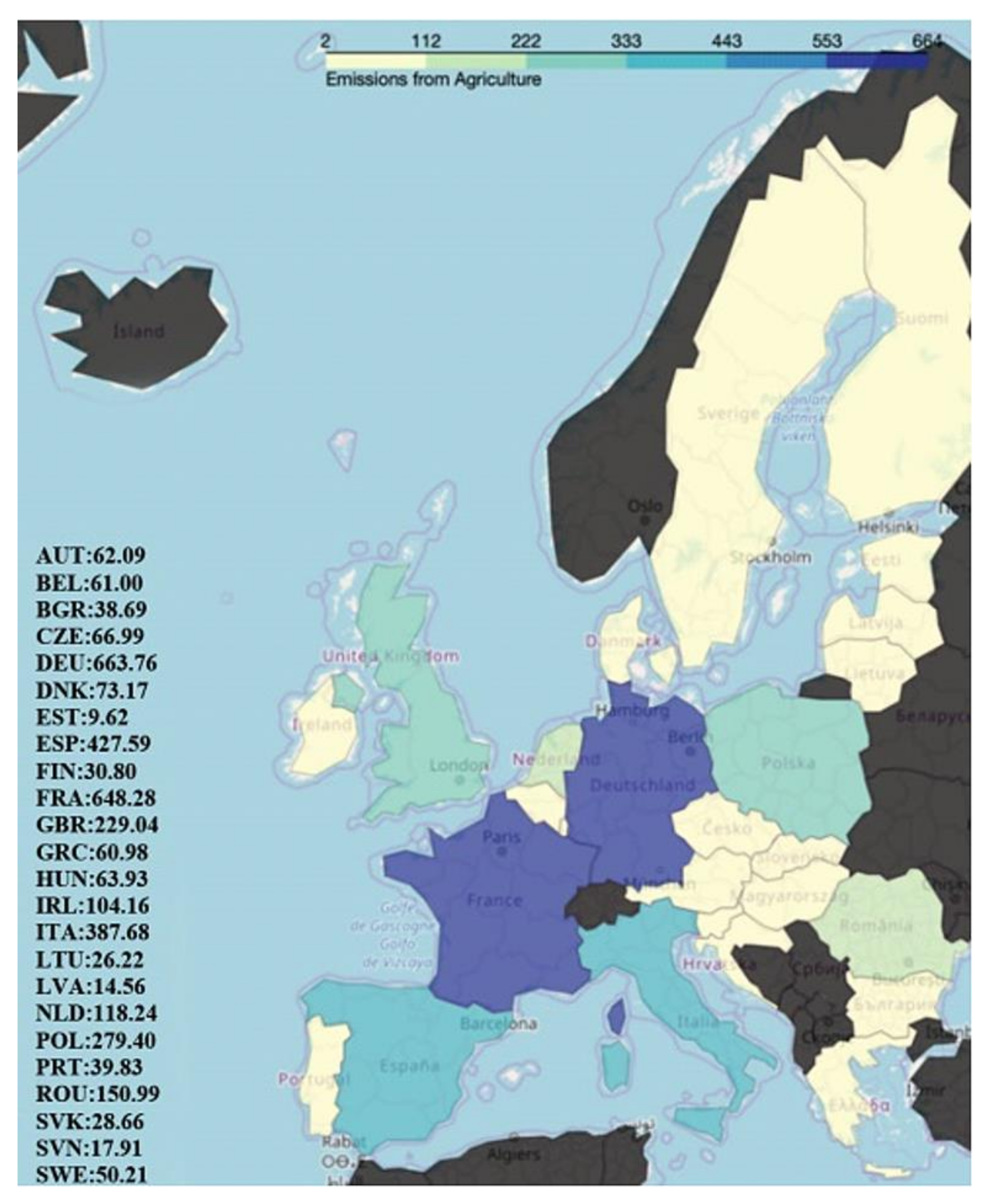
The situation related to fertilizers used in the agricultural sector for each of the EU member countries is generally synchronized with both the level of ammonia (NH₃) (Figure A14) and CO₂ (Figure A15) emissions, because of the agricultural production.

However, from the Eastern EU countries, Poland and Romania report the highest amount of ammonia (NH₃) emissions, but even so, significantly less than France, Germany, Italy, and Spain (Figure A14). Poland registered the highest amount of CO₂ emissions (Figure A15) from the Eastern EU countries, akin to the fertilizer situation (Figure A9).

Regarding Ireland, the fertilizer usage value is considerably higher (Figure A9), although both the ammonia (NH₃) (Figure A10) and CO₂ (Figure A11) emissions registered low values. This may indicate a possible better sustainable fertilizer use technology, compared to rest of the EU countries.

Direct payments are considered the main instruments, which support farm income and, therefore, contribute to rural vitality. However, according to the European Commission, despite the increase in size and the improvement of productivity, many farms depend heavily on direct payments. However, concomitantly, direct payments ensure sustainable farming through economic viability.

The largest amount of direct payments is attracted by agriculture farmers from Western EU countries, such as Germany, France, Spain, Italy, and United Kingdom (Figure A12). In Eastern EU countries, Poland and Greece records the highest values of direct payments (Figure A13).

This situation is generally reflected by the registered status of agricultural entrepreneurial income, where Eastern EU countries registered the lowest results (Figure A13). The direct payments support farm income and also, eliminates possible uncertainties related to agriculture economic activity.

Thus, a possible increase of these countries capacity to attract direct payments will possibly lead to more consistent agricultural entrepreneurial income, increase agricultural entrepreneurial market competitiveness, and facilitate the intention of farmers to adapt, considering present situation related to climate change. Additionally, ensuring a fair income for farmers is one of the objectives proposed in the CAP reform.

According to [70], economic development theorists and practitioners have long focused attention on the question of the impact of food prices on poverty in developing countries. However, long periods of low agriculture prices can reduce return and increase rural poverty. Additionally, in low-income countries, heavy taxation of agriculture through lower commodity prices might have contributed to extensive rural poverty [71]. However, it is difficult to estimate the effect of changes in food prices over poor households, since this is influenced by the level of dependence on agriculture production as a source of income.

Both the degree of rural poverty (Figure A14) and the consumer price evolution of food products (Figure A15) records the highest values, generally, in Eastern EU countries. This reveals that the rural economy is strongly related to agricultural production, as high food prices may affect affordability of consumption basket components, return of agriculture activity, as well as labor demand and wages in the agriculture sector.

The highest differences between rural employment rate for males versus females are recorded in Italy and Greece (Figure A16 and Figure A17). However, the agriculture employment rate is generally influenced by the economic performances of the sector. Thus, in order to improve production and performance and to decrease poverty, research and development activities are important. A previous study [72] emphasized that the returns to agricultural research and development have been large. The underinvestment in public research and development activities can eventually lead to the impossibility of satisfying of aggregate demand for food, increasing food prices and rural poverty. In Eastern EU, the research and development investments are considerable low, compared to Western EU countries (Figure A18). If public investments in research and development will increase in Eastern EU, these countries will growth in importance as producers of agricultural innovations and will improve their agriculture production performance.

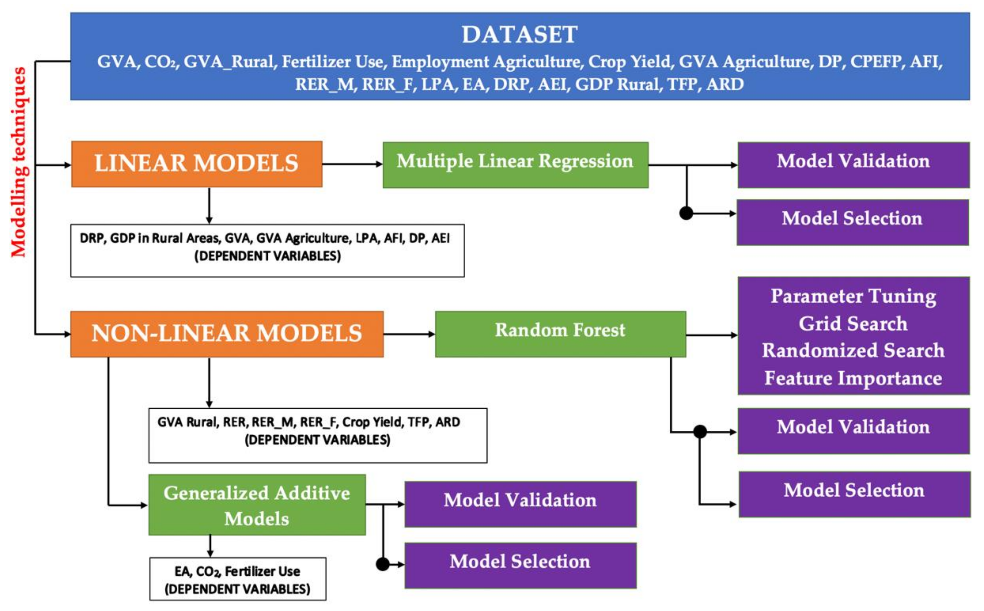
The current research developed analytical framework took into consideration four main dimensions for describing the intricacies of the EU Agricultural and Rural Environment in the CAP context: (a) rural, (b) emissions, (c) macroeconomic, and (d) financial.

Each dimension is described by a set of parameters, respectively a set of predictive models. The developed models aimed to accurately predict the targeted parameters, but also to provide a glimpse in formally understanding, which are the most relevant parameters when determining targeted indicators.

3.2. The ‘Rural’ Dimension

The rural dimension is described by the following six parameters: DRP, GVA_Rural, RER_M, RER_F, RER, and GDP (rural GDP per capita). Predicting these parameters involved the development of both linear models and non-linear random forest models as not all parameters could be described through linear regression modelling.

According to the Ministry of Public Works, Development and Administration—MLPDA (Strategy for the development of the agri-food sector in the medium and long term 2020–2030), the level of national incomes in rural areas represents approximately 16.6% of the European average, in the context of an average income ranked lower than the European one.

The phenomenon of rural poverty can be explained in terms of the advanced age of the rural population, a low degree of employment, a limited employment opportunity and the low wages. An important influence on the level of rural poverty has the investments in the agricultural sector, through European and national financing instruments, also, the research—development activity is stimulated by the European regional development policies. Direct payments could positively stimulate the rural economic development, the GDP growth, with implicit effects on reducing the rural degree of poverty.

The degree of rural poverty is an important aspect to be understood, its reduction bringing benefits for the deceleration of the rural-urban migration process, conducting to a lower pressure on government to provide additional spending on services, such as sanitation, health, and education in urban areas.

In this research, it was possible to model the degree of rural poverty indicator through linear modelling, by using best subset selection technique to choose the set of independent variables. The equation describing the DRP indicator is the following:

$$\begin{gathered} Ln\left(DRP\right)=9.07+0.22Ln\left(Employment Agriculture\right)-0.13Ln\left(GVA Agriculture\right)+0.07 Ln\left(DP\right) \\ -0.57Ln\left(GDP Capita Rural\right)+0.13Ln \left(ARD\right)-1.11Ln\left(RER\right) \end{gathered}$$

(2)

The linear regression model presented above shows good accuracy metrics, having the S-value at 0.18, the adjusted R-sq at 77.99% and the predicted R-sq at 76.66%. The result of the analysis shows that the degree of rural poverty decreases with the increase of: The Gross Domestic Product per capita in rural areas (−0.57%), the employment rate (−1.11%), the of the gross value added (−0.13%), with the values of 0.57, 1.11, respectively 0.13%.

It can be noticed that the ‘Rural Employment’ parameter was identified as an important predictor of the model, an increase of its value by 1% resulted in a 1.11% decrease in the rural poverty Equation (2). Additionally, gross domestic product per capita is considered the second parameter, regarding its importance in determining the degree of rural poverty Equation (2). Thus, this emphasizes that a sustainable economic growth will be achieved by increasing both gross domestic product per capita and gross value added of the agriculture sector Equation (2), since they significantly influence the degree of rural poverty Equation (2). Therefore, rural poverty is responsive to economic growth in rural areas. Dollar and Kraay (2001) [73] emphasized that economic growth may reduce poverty by raising the incomes of everyone in society, including the poor. Additionally, another study [74] revealed the importance of economic growth in reducing poverty, pointing out, also, the importance of the inequality variable.

In [75], the authors, after analyzing the determinants of rural poverty in 32 developing countries, also identified that the gross agricultural value added, and rural employment are important factors contributing to alleviating poverty in rural areas. Besides these two parameters, the authors also identified the government policies for reducing systemic discrimination against ethnic minorities, the encouraging tourism where possible and the programs designed to assist the irrigation of croplands as important variables that influence rural poverty degree. However, considering Equation (2), the agriculture research and development and agriculture employment rate negatively influence the degree of rural poverty. This may be due to bad agriculture research management, which targets the fundamental area, rather than applicative area. Additionally, a high employment rate in the agricultural sector can decrease the average income, as well as labor productivity. A poor agriculture research management will decrease the productivity because of low degree of technical and technological development and, therefore, increase the employment rate.

The reduced DP importance can be justified by the fact that CAP does not clearly define their amount for each region, according to a large framework of specifications. This is mentioned by other authors [76], which underline those specific guidelines should be define separately, for each geographic region, to increase the efficiency of CAP towards a better sustainable development. Other studies [77] emphasize that agricultural payment tools improve the production capacity of cultivated land, a situation which will lead to the increase of labor productivity and a decrease of RER. Thus, models that imply payment tools should be considered together with flexible policies, which can relax the decision-making process related to various specific aspects within limited time-periods. However, there are studies [77] which emphasize that payment tools should be used together with regulatory tools in order to establish a hybrid system, which aims to maximize the positive impact.

According to [78,79], over 80% of farms in the EU are represented by family farms; therefore, DP are being infused into local economies on a much higher scale, compared to the financial support received by industrial corporations, which in a form of dividends may be allocated out of EU. Therefore, DP can be considered as tools of fostering the national economic growth and can accentuate the differences between the EU member states. Hence, prediction models, which imply the DP as an independent variable, are important to for considering the new CAP programming period, since, according to other authors [80], they are considered the main funding issue and, therefore, creating fairer criteria for the distribution of financial envelopes of DP between the EU member states is proprietary. Thus, prediction models will offer superior performance, compared to classical arithmetic-based rules standardized by EC [81].

GDP per capita in rural areas shows how much economic production value can be attributed to each individual citizen living in rural settlements, being also a prosperity measure, since it can be translated as a measure of wealth. The GDP per capita in rural areas is an important parameter to be measured and forecasted. Indeed, it is also part of the explanation why many rural populations flow to non-agricultural sectors and urban areas [82].

For the current study, the ‘GDP per capita in rural areas’ (GDP) indicator modelled using a multiple linear regression, with the following obtained model:

$$\begin{gathered} Ln\left(GDP\right)=7.18+0.08 Ln\left(Fertilizer Use\right)+0.18Ln\left(Employment Agriculture\right)-0.17 Ln\left(CPEFP\right)+ \\ 0.18Ln\left(LPA\right)-0.12Ln \left(EA\right)+0.16Ln\left(ARD\right)-0.37Ln\left(DRP\right) \end{gathered}$$

(3)

The above model has good accuracy metrics: S value 0.14, adjusted R-sq 87.19%, and predicted R-Sq 85.84%. The model shows how the set variables influence the rural Gross Domestic Product per capita in rural areas.

Thus, a positive impact for the use of fertilizers in agriculture (0.08%), the employment agriculture rate (0.18%), the labor productivity in agriculture (0.18%), and the agriculture research and development (0.16%) variables, in addition to a negative impact of the consumer price evolution of food products (0.17%), ammonia emissions from agriculture (0.12%), and the degree of rural poverty (0.37%) variables on the gross domestic Product per capita in rural areas, can be observed.

The rural GDP per capita is influenced by the size of employment rate in agriculture—Equation (3). With the increase in the number of people employed in rural areas, there is also an increase in the value of rural GDP and, implicitly, a reduction in the degree of rural poverty. Several authors [64,83,84,85,86] have emphasized the importance of increasing employment in rural areas and encourage CAP to increase this initiative as a remedy for social exclusion, depopulation of these areas, and the income gap, in order to achieve high sustainable agriculture. Additionally, according to Equation (3), the ARD and EA directly influence the GDP situation, which can confirm the finding of other authors [87,88,89] related to the relation between human capital, as well as its qualification and education and income of agricultural population.

The Agriculture Research and Development activities, strongly stimulated and financed by the EU, in the period between 2014–2020, together with efficient and well-implemented public policies and good agricultural practices will stimulate the efforts for obtaining new technologies, optimal production systems, in relation to local characteristics, the know-how transfer, promoting cooperation and innovation, increased agricultural productivity (influenced also by the efficient use of fertilizers), and implicitly the increase of rural GDP per capita.

However, considering the relationship between GDP per capita and fertilizer use, as well as ammonia emissions from agriculture, it seems that environmental sustainability significantly influences the gross domestic product per capita. Thus, the use of fertilizers promotes the increase of crop productivity and, therefore, the economic growth. This can only be possible if sustainable fertilizer administration technologies are used (ammonia depth soil injections), limiting, therefore, ammonia emissions.

The rural GDP formation is also conditioned by the consumer price evolution of food products. While incomes of the rural population remain constant and the prices increase (regardless of the form of inflation, i.e., increases in production costs or demand for products and services), consumption automatically decreases, as well as the incomes of companies offering products and services, and there is a decrease in their financial and economic performance, with direct negative effects in the formation of the national GDP. The effects can be even stronger in terms of lower wages in rural areas.

The above findings are confirmed in studies, such as [90,91] where the authors investigate the relationship between both ‘relative GDP share of rural areas’ and ‘relative GDP share of agriculture’ versus the agricultural employment rate. In [91], based on a sample of ten Central and Eastern European countries, the authors identify a strong relationship between the GDP share of agriculture and agricultural employment rates, their findings suggest that agriculture may play a role in lowering the prevailing rates of high unemployment. Moreover, in [90], the authors present the main aspects of the Common Agricultural Policy (CAP) emphasizing on the strong relation existing between agricultural employments and rural areas GDP share, inside the European Union (EU) member states

As presented in Figure A5, there are many European countries where rural environment added value (GVA_Rural) has a significant share in the overall country GVA, e.g., Austria, Germany, France, Italy, Portugal, Romania, Slovenia. In [92] the authors present the economic importance of the private rural sector, such as the contribution of businesses to Gross Domestic Product. Their findings reveal that, besides the contribution to the overall gross value added, the rural businesses are improving the local resilience in both direct and indirect ways. As direct contributions, the creation of local employment and local product and service delivery can be mentioned, while for indirect contributions, the added value of primary business activities can be mentioned.

The current research models the ‘GVA_Rural’ parameter through a random forest model with base model (BM) accuracy at 89.27%, random search accuracy (RS) at 92.02%, grid search accuracy (GS) at 92.28% and model validation (MV) accuracy at 65.07%. After performing the feature selection analysis, it was concluded that, according to their weights, the following five parameters were the most important (contributed the most) to the prediction of the Rural GVA indicator: 0.24 for EA, 0.23 for DP, 0.11 for CO₂, 0.05 for GVA Agriculture, and 0.01 for Employment Agriculture.

As it can be observed, the GVA_Rural prediction depends mostly on EA, DP, CO₂ and GVA Agriculture. According to the above weights, it can be stated that there is a connection between the CAP direct payments and the gross value added of the rural environments. The ‘DP’ indicator has second weight in the model, its contribution to the dependent variable prediction being significant. The ‘Ammonia Emissions’ parameter displays the higher weight in the model. This confirms that agriculture plays an important role in the development of rural communities as most of the ammonia emissions are related to agricultural activities. Besides ammonia emissions, it can be observed that CO₂ agricultural emissions ranks third, enforcing the hypothesis that for the European rural environment development, agriculture plays a pivotal role. An intensive agriculture, which implies intensive fertilizer administration, will have a direct and instant effect on rural GVA, through improving agriculture productivity. However, considering Equation (3) and the above weights, it can be recommended to use direct payments to invest in upgrading the fertilizer technologies, since environmental sustainability will influence economic growth.

Rural areas are different in accordance with social and economic dimensions- they are not homogenous. Traditionally, the population density was used for the definitions of rural areas in Europe. As defined by EUROSTAT, rural areas are defined as those with a population density of less than 100 inhabitants/km².

The EC communication entitled “The Future of Rural Society” (EC, 1998:28-29) identifies three standard problems of rural areas: the pressure of modern life, rural decline and job finding/rural employment and difficulty to reach very marginal areas. Additionally, according to their extent of integration within the national economy, rural areas are distinguished as: integrated rural areas—with a growing population, an employment basis in the secondary and tertiary sectors, but with farming as key activity of use of land, intermediate rural areas—relatively distant from urban centres, with a varying mix of primary and secondary sectors—larger scale farming operations and remote rural areas—with the lowest population densities, often the lowest incomes, and an older population, which depends heavily on agricultural employment.

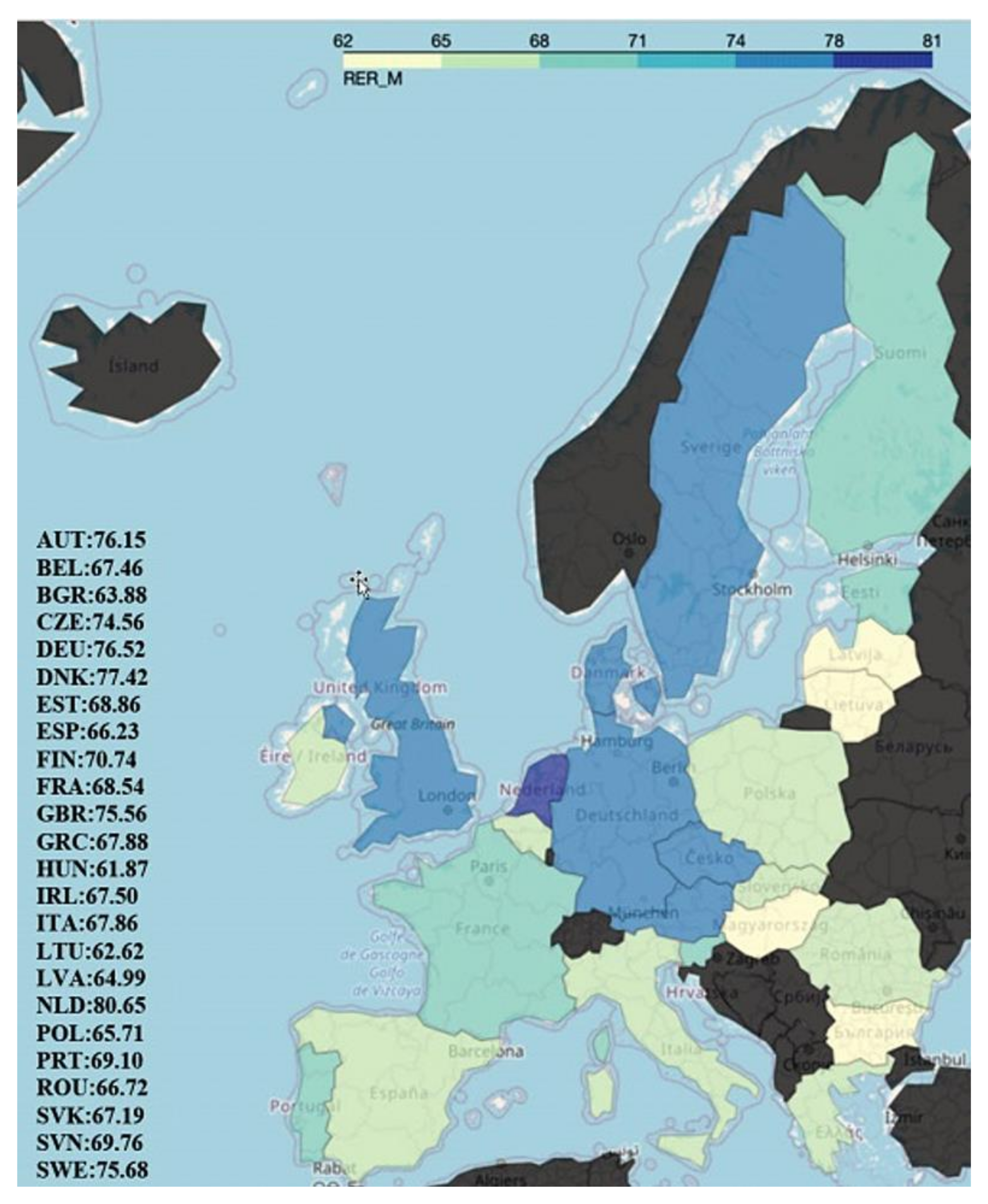
The current research presents a set of three models describing the European rural employment rates based on the available dataset containing CAP related indicators. Thus, based on the dataset presented above, this study considered the following rural employment related parameters: (a) the overall European rural employment rate, (b) male rural employment rate, (c) women rural employment rate.

The following figure displays a six-year average of the aforementioned parameters for each of the European states:

As it can be noticed from Figure 5, the rural employment rate for women in rural environments is noticeably lower than the male one. Among all analyzed countries, Greece, Italy or Romania present the highest difference between the previous mentioned indicators. Additionally, it is easy to spot the countries with the highest rural employment rate, namely: Germany, Denmark, The Netherlands, Sweden, and the UK.

According to [93], 40 years ago throughout Europe, women in rural areas had fewer employment opportunities, compared to both men in rural areas and women in urban areas. These days it is still difficult to provide a picture of the average employment situation of rural women, as employment prospects differ enormously by age, marital status, family stage or country. However, currently, the rural employment gap between man and women narrowed a lot for several EU countries Denmark, Finland, Netherlands, and Sweden.

The present study aimed to formalize, based on the available dataset, the various existing perspectives on rural employment rates. Therefore, this research modelled all three rural employment rate parameters (RER, RER_M, RER_F) through a non-linear random forest approach, obtaining three different models with the following characteristics:

• The overall ‘Rural employment rate’ (RER) model has the base (BM) accuracy at 97.79%, random search accuracy (RS) at 97.86%, grid search accuracy (GS) at 97.82% and model validation (MV) accuracy at 93.53%. The feature selection analysis shows that, according to their weights, the following five parameters were the most important for the prediction of the Rural_GVA indicator: 0.68 for DRP, 0.41 for GDP per capita in rural areas, 0.20 for RER_M, 0.18 for EA, and 0.14 for GVA_Agriculture.
• The model describing RER_M parameter has a base model (BM) accuracy at 98.14%, random search accuracy (RS) at 97.87%, grid search accuracy (GS) at 97.84% and model validation (MV) accuracy at 97.65%. By performing the feature selection analysis, it was identified that, according to their weights, the following five parameters were the most important for the RER_M indicator prediction: 0.49 RER_F, 0.21 for GDP, 0.20 for DRP, 0.10 for GVA Rural, and 0.01 for CPEFP
• The RER_F random forest model also displays very high accuracy metrics. Its base model (BM) accuracy is at 98.60%, random search accuracy (RS) at 98.68%, grid search accuracy (GS) at 98.60% and model validation (MV) accuracy at 96.01%. The most important parameters are described by the following weights: 0.68 for DRP, 0.41 for GDP capita in rural environment, 0.20 for RER_M, 0.18 for EA and 0.14 for GVA_Agriculture.

As it can be noticed, for the prediction of the overall rural employment rate all five parameters contributed significantly, especially the degree of rural poverty and GDP per capita in rural areas (as implied by the weights presented above). The description of the relationship between the degree of rural poverty and rural employment rate was found in [94], where the authors show that the rapid growth of the agricultural production and income of the farm employees is the dominant means of reducing rural poverty. Additionally, according to the authors, large-scale commercial farms show little impact on rural poverty reduction, as compared to areas dominated by small commercial farms that are providing jobs for more communities.

Regarding the male rural employment rate, the most significant parameters were the women employment rate and the rural gross domestic product per capita. This implies that a possible relation exists between the rural rate of employment for man and the rural rate of employment for women.

The women rural employment rate model parameters are all contributing significantly to predicting the dependent variable (RER_F), especially the degree of rural poverty and GDP per capita in rural environments. As the model implies, the value for the degree of rural poverty strongly influences the accuracy of the model when predicting women rural employment rate. In [95], the author, after having analyzed the change in trends of women’s unemployment and poverty rates, also noticed their interrelationship. Thus, there are studies [95,96] which clearly highlights that unemployment is one of the main reasons of poverty and the women unemployment rate in 28 countries of the EU, is lower than men; however, their risk of poverty rate outweighs the indicator of men.

3.3. The ‘Environmental’ Dimension

In the context of the current research, the ‘Environmental dimension was described by using three parameters: EA (ammonia emissions in agriculture), CO₂ emissions, and Fertilizer_Use, based on studies, such as [97], which come from agriculture. Additionally, in [98], it is shown that agricultural activities represent the major CH₃ source and effective methods are needed to quantify and mitigate these emissions, while also understanding the current factors that are influencing it. European progress in reducing agricultural emissions is not as high as needed to be [99,100], the air pollution is constantly increasing in countries with developed agricultural systems [101,102].

The current research emphasizes that the agricultural sector’s ammonia reduction methods seem to be directly affected by the agricultural investments, such as CAP direct payments. Based on the GAM model presented in Equation (4), these investments have a significant impact over the ammonia emissions Equation (4). Besides direct payments, predictors, such as employment in agriculture, and fertilizer use, gross value added of the rural environment or GDP display an interpretable influence over the agricultural emissions. For the current research, after applying the generalized additive model technique (GAM), the emissions in agriculture parameter were explained by the following model, where s represents the spline function associated to each predictor:

$$\begin{gathered} \left(EA\right) ~ s\left(DP\right)+s\left(DRP\right)+s\left(Employment\_Agriculture\right)+s\left(Fertilizer\_Use\right)+s \left(GDP\right)+s\left(GVA\right) \\ +s\left(GVA\_Rural\right)+s\left(LPA\right) \end{gathered}$$

(4)

Initially, the model was trained with all the available predictors, but the final version included only the significant ones (presented in Figure 6).

The model presented in Equation (4) is described by excellent accuracy metrics, having the adjusted R-sq at 98.20% and as it can be observed, the direct payments parameter fit values shows that higher values of DP have a clear negative influence over the ammonia emissions, after exceeding a specific threshold.

For lower direct payments, the influence over the emissions in agriculture is positive, but as the DP values increase, the effect over the EA starts to reverse. It could be assumed that when the direct payments are higher, they are also used for purchasing improved fertilizers. All the significant parameters have a positive effect over the EA, but with several peculiarities.

For example, the influence of the employment in agriculture parameter over EA presents a sudden increase for values between 10–20%. The GDP’s influence decreases for high GDP values (highly developed countries being able to use the latest agricultural research products), while for the gross value added by the rural sector or for the fertilizer use, the model presents a direct ascending trend of their positive influence over the EA. In [103], the authors emphasize that the mitigation of the greenhouse ammonia emissions from the agriculture would be possible if a technological path is followed.

Technology leads to a higher productivity and, as Figure 6 presents, even a small increase in agricultural labor productivity is associated with lower ammonia emissions, similar with the high LPA values.

The environmental dimension includes the CO₂ emissions in the agriculture as several studies showed that agricultural activities are responsible for the overall increase of the CO₂. In [104], the conversion of different ecosystem for the agricultural usage is presented as one of the causes for CO₂ emissions.

Also, [105] shows that agricultural activities are sources of greenhouse gases, such as CO₂, CH₄, and N₂O and reliable quantifications should be obtained to assess the necessary budgets for land-use management and for climate research.

Like ammonia emissions, there are parameters related to industrialization, agricultural research and development, rural development, specific policies, or know-how improvements that are influencing CO₂ emissions. According to the current research, CO₂ emissions were also modelled by using a generalized additive model.

Thus, Equation (5) displays the most significant predictors over the CO₂ agricultural emissions.

$$\begin{gathered} \left(CO2\right) ~ s\left(ARD\right)+s\left(DP\right)+s\left(Employment\_Agriculture\right)+s\left(Fertilizer\_Use\right)+s \left(GDP\right)+s\left(GVA\right) \\ +s\left(GVA\_Agriculture\right)+s\left(GVA\_Rural\right)+s\left(LPA\right)+s\left(RER\right)+s\left(TFP\right) \end{gathered}$$

(5)

The above model has excellent accuracy metrics (adj R-sq: 97.45%); as it can be observed (Figure 7), each predictor has a positive influence on the dependent variable, meaning they all contribute to the overall increase of the CO₂. However, their influence is not linear. The direct payments display a slow increase for low DP values and a stronger one for high DP values. The ‘fertilizer use’ and ‘gross value added’ parameters clearly influence the CO₂ emissions, higher values also meaning higher CO₂ values.

We can observe three cases (GDP, GVA_Agriculture, LPA) where the influence of predictors over CO₂ emission decreases as their value increases. The high GDP values reflects the developed countries, which are continuously aiming to reduce greenhouse gas emissions, while high values of GVA_Agriculture and LPA reflect the countries with developed agricultural systems, which are using modern greener technologies to increase agricultural productivity.

Fertilizers are used extensively by farmers, still, their use is expensive and can harm the environment. In [106] the authors describe how the excessive use of fertilizer generated environmental degradation and how fertilizer use decreased with the increase of farm size, as in small farms a very low machinery level inhibited the precise fertilization.

In the current research, the fertilizer use modelling was performed by using a non-linear generalized additive model Equation (6), as the linear modelling displayed low accuracy metrics.

$$\begin{gathered} \left(Fertilizer\_Use\right)~ s\left(Employment\_Agriculture\right)+s\left(GVA\_Agriculture\right)+s\left(GVA\_Rural\right)+s\left(RER\right) \\ +s \left(TFP\right)+s \left(Crop\_Yield\right) \end{gathered}$$

(6)

The ‘Fertilizer Use’ prediction model showed high accuracy metrics, with an Adj-Rsq value of 0.97 and according to the determined feature significance, the most important parameters for explaining the variance of the ‘fertilizers use’ dependent variable are: Crop_Yield, Employment_Agriculture, GVA_Agriculture, GVA_Rural, rural employment rate, and total factor productivity.

As noticed from Figure 8, the total factor productivity (TFP) and the Crop_Yield predictors display the existence of a clear relation relative to the dependent variable ‘fertilizer use’.

TFP represents the ratio between output to inputs [107], more specifically the rate at which the ratio of outputs to inputs changes over time [108]. If the production changes came from a greater input use (e.g., more fertilizers, workers, and/or land), the change in TFP would be zero. Thus, as noticed in the above figure, a higher TFP value is related to lower values of fertilizer use. Higher TFP values are related to technical change and efficiency improvements, being usually associated with agricultural systems based on improved plant varieties, agricultural mechanics advances or irrigation expansion and less on quantity of used fertilizers. Therefore, if a country has higher total factor productivity values, it can yield higher output with the same resources. Market imperfections could induce an increase of flexibility related to agriculture products, determining the decrease of prices if market offer for agriculture products increase and, therefore, if productivity increases, as was reported in other study [64]. This hypothesis is also confirmed by other authors [109] who emphasize that constant effort to improve factor productivity by adopting new technologies might not induce positive results in terms of farms profitability. However, according to other authors [110], most agrarian transformation is focused on improving farming productivity and, on long-term, this will generate agriculture labor transfer through other economic sectors. Therefore, according to [111], high TFP generates low agriculture employment rate. Additionally, another study [112] concluded that moderate cuts in unconditional DP would have no negative farm employment effects, underlying the low impact of these payments on agriculture employment rate and revealing that economic developments outside agriculture have, via the general wage level, the most pronounced effect on labor use in the farm sector. However, since the impact of subsidies on agricultural employment rate was found to be either positive [113], mixed [112], or negative [114], a strong need for using prediction modeling techniques is needed to define specific frameworks for proper efficient DP inputs, considering indicators related to both direct and indirect effects.

In predicting the ‘Fertilizers Use’ value, the fit values of the spline function associated to ‘Crop Yield’ parameter shows that for most of the cases the crop yield increase is associated with an increase of the ‘fertilizer use’ parameter.

The importance of the ‘Fertilizer Use’—‘Crop Yield’ relation is presented in several studies. In [115], the authors show that the use of pesticides and mineral fertilizers has improved crop yields but also contaminated food and the environment. Based on their findings, the fertilizer and pesticide consumption continuously increased. Additionally, in [116], a research that estimates the role of agronomic inputs in cereal yield improvements, the authors clearly show the role of fertilizer and modern seeds in boosting yields. Besides crop yield and TFP, the ‘rural employment rate’ and the ‘employment in agriculture’ fit spline values describe a situation similar to the finding presented in [117], where the authors showed that farmers use less fertilizer in a context where the rural employment rate is high.

3.4. The ‘Macroeconomic’ Dimension

The ‘Macroeconomic’ dimension, presented in this study, is described by the following five parameters: GVA_Agriculture, Crop_Yield, TFP, GVA, LPA.

C.A.P. represents the starting point for the planned policies on climate and energy for 2030. Through them are imposed the objectives of reducing emissions by 40% by 2030 and the participation of the agricultural sector in achieving this goal.

Increasing the added value in agriculture, at national and regional level, together with the transition to a sustainable agricultural production, are aspects intensely monitored by the European Union. European funds are dedicated, managed by the Agency for Financing Rural Investments Institution, subordinated to the Ministry of Agriculture and Rural Development (MADR), with attributions of technical and financial implementation of the National Rural Development Program 2014–2020.

According to [118], in Europe, agriculture accounts for more than 47% of the total territory. In recent decades, European agriculture has experienced a continuous decrease in the number of farms, while the farm size shows a tendency towards larger holdings. According to the authors, a similar tendency was observed also for the share of agriculture in the gross value added (GVA), but with some differences between European regions, see Figure A5.

The growth of the gross value added in agriculture (GVA Agriculture) depends largely on a country’s level of development and it is correlated with various exogenous factors. A stable economic environment, for example, which favors the investments, will create the premises for the development of the agricultural sector. In other words, the conditions in which the existing economic agents in agriculture carry out their activity in stable conditions from an economic, political, legislative point of view, they can participate in increasing of the added value at national level.

The current research identifies an accurate multiple linear regression model (S-value 0.45, adjusted R-Sq 85.44%, predicted R-sq 85.09%) for determining the gross value added of the agricultural sector, see Figure A7.

$$Ln\left(GVA Agric\right)=-4.22+0.32 Ln\left(DP\right)+0.14Ln\left(LPA\right)+0.54 Ln\left(EA\right)$$

(7)

An important aspect, revealed by the above model, is the importance of the direct payment’s indicator, that is a 1% increase of the direct payments would lead to a 0.32% increase of the GVA agriculture.

As the above model shows, the GVA_Agriculture parameter is positively influenced by the rest of the variables included in the model: Labour Productivity in Agriculture (LPA) by 0.14% and the Ammonia emissions from agriculture by 0.54%.

In [118], the authors investigate the factors that govern the differential performance of agriculture across the EU-27 countries by using a machine learning technique, respectively k-means clustering method, identifying a strong relation between agricultural labour productivity, specifically agricultural investments, and the economic performance of the sector.

The development of agriculture sector implies high production intensities, possibly due to extra-investments, as direct payments, made for both improving labour productivity and increasing the use of fertilizers, which will promote growth.

The overall Gross Value-Added parameter can be expressed through a multiple linear regression model with very good accuracy (S value 0.20, adjusted R-sq 97.83%, predicted R-sq 97.67%)—see Equation (8).

$$\begin{gathered} Ln\left(GVA\right)=-4.37+0.09 Ln\left(C{O}_2\right)+0.10Ln\left(GVA rural\right)+0.31 Ln\left(Fertilizer Use\right)- \\ 0.35Ln\left(Employment Agriculture\right)+0.67Ln \left(GVA Agriculture\right)+0.17Ln\left(DP\right)+1.30Ln\left(RER\right) \end{gathered}$$

(8)

According to the above model, the overall gross value added is positively influenced by several parameters. According to these, an increase in the rural employment rate, or agricultural CO₂ emissions, or agricultural gross value added or fertilizer use or direct payments would lead to an increase of the gross value-added indicator. The only negative influence comes from the ‘Employment in Agriculture’ parameter, that could be explained by a significant agricultural employee reconversion to services or industrial field. This explanation is sustained also in [119], where the authors identifies that the number of agricultural co-operatives has been continuously decreasing, even they are still providing job opportunities.

The labor productivity is determined by comparing the labor cost with the total labor efficiency. In agriculture, labor productivity (LPA) refers to the number of units of output(s) produced per unit of labor used in the process of production. It is an indicator that is determined by dividing the quantity of output by the total units of labor used. Assessing the quantity of labor input involves the number of active workers and the number of time units (hours, days, and months) worked.

According to [120] agricultural labour productivity plays an important role in defining the competitiveness of the sector, contributing to the overall economic development. Thus, the authors examine labour productivity differences in the Greek agricultural sector, by analysing the factors that determine the productivity of the sector and investigating the relation between productivity and its determinant factors, determining two basic factor categories: (a) factors linked to the structure of the agricultural enterprises—used productive (human and fixed) capital, technology, productive dynamism, scale returns, (b) factors related to the land and the natural environment.

In [121], the authors position LPA as one of the methods that could be applied by farmers to profit from the economic growth in their society: (a) increase the yields of their crops and animals, (b) switch to the production of high value products (for which there is an increasing demand in the market), (c) increase the labour productivity on their farm, and (d) find non-farm sources of income for some or all of their family members. Increasing the LPA is also important as many farmers are aware that with the increasing average income in their country the proportion of the labour force, which can find employment in agriculture decreases.

Also, as presented in [122] high and unstable food and agricultural commodity prices, environmental constraints and concerns about population growth pushed the agriculture production on national policy and research agendas that requires relevant and accessible monitoring indicators—LPA being one of them.

The current study presents a linear modelling describing the LPA parameter. The model Equation (8) has very good accuracy metrics having S value at 0.24, adjusted R-sq 92.67% and predicted R-sq at 92.01%.

$$Ln\left(LPA\right)=-1.89+0.14 Ln\left(GVA\right)-0.06 Ln\left(GVA rural\right)+0.86 Ln\left(AFI\right)+0.59Ln\left(RER\right)$$

(9)

According to the above equation the Agricultural Factor Income parameter displays a strong influence, as a 1% AFI increase will lead to a 0.86% LPA increase, with the rest of the parameters remaining constant. Additionally, the rural employment rate displays a strong positive influence as the value of LPA will increase by 0.59% for a 1% RER increase.

The relationship between remuneration and productivity of labor factor (at the level of the agricultural sector) is presented in detail, both analytically and empirically by [123]. Based on an optimal solution of the income maximization problem, they derived the determinants of remuneration of the labor factor, i.e., labor productivity and subsidies.

However, considering Equation (8), it can be stated that the GVA influence positively the labor productivity in agriculture, compared to GVA Agriculture. Since agriculture is considered a complex sector, this implies the establishment of a series of direct relations with other sectors. Therefore, the labor productivity is mostly related to technological factors, but can be also influenced by the technical progress of the economy. Therefore, using automatized equipment for technological operations related to different crop production stages can involve low number of employees and, respectively high labor productivity. However, the automatization of agriculture production cycle may raise problems related to rural employment and, therefore, may affect rural GVA. This can explain the negative relation between LPA and rural GVA, revealed by Equation (8).

The crop yield represents a measurement of the amount of agricultural production harvested—yield of a crop—per unit of land area, being an important parameter to understand because it helps optimizing food security programs, also explaining cost variation for different years.

Modelling crop yield and crop production is necessary at EU and member state level for providing to CAP decision makers timely information needed for a rapid decision-making during the growing season. Furthermore, estimating the crop production is useful in relation to trade, development policies and humanitarian assistance linked to food security.

In [124], the authors also propose an analytical framework allowing estimation of the effects of the new instrumentation of the CAP in the arable crop sector—crop yield, price cuts and compensatory payments.

The ‘Crop_Yield’ parameter could not be modelled with linear modelling techniques and a random forest model was used.

The model describing Crop_Yield parameter has a base model (BM) accuracy at 92.20%, random search accuracy (RS) at 91.80%, grid search accuracy (GS) at 91.85% and model validation (MV) accuracy at 88.14%. By performing the feature selection analysis, it was identified that, according to their weights, the following parameters were the most important for the Crop_Yield prediction: 0.36 LPA, 0.30 Fertilizer Use, 0.12 for GVA_rural, 0.04 for DRP, and 0.02 for CO₂. However, crop production is not related to DP. This is also reported by other authors that emphasized the low efficiency of CAP support regulations about the financial flow volume, pointing out the impact of relatively high support for large holdings on discouraging the boosting of productivity [125]. There are studies [126] which characterize subsidies as both negative and positive mechanisms for improving agriculture farm behavior, as they can encourage farmers to expand production through activities that they would consider too risky in the absence of guaranteed income from DP, while, at the same time, as negative aspect, farms production structures distortions can appear. However, since farm overinvesting can be considered a risk of DP, an entrepreneurial training for transferring know-how within facilities owners must be considered to be integrated in future CAP.

According to the above weights, the most important factors in determining crop yield value are LPA and the fertilizer use. Both factors contribute most to the model accuracy, this current study confirming previous models. Such an example can be found in [127], where the authors apply a different machine learning approach, that is a multilevel logistic regression for investigating the labor productivity of the six main agricultural systems across European NUTS2 regions, mentioning the strong relationship existing between LPA and crop yield. In [128] the authors emphasize that the benefits of nutrient inputs are often minimized in discussions of potential risk. The purpose of their research was to examine existing data and approximate the effects of nutrient inputs, specifically from commercial fertilizers, on crop yield. A total of 362 seasons of crop production were included in the long-term study evaluations and the results of their investigation indicated that at least 30 to 50% of crop yield is attributable to commercial fertilizer nutrient inputs.

Hence, intensive agriculture, associated to high values of crop yield, will generate high LPA, due to a high automatization degree of all processes included in crop culture technology and, also, will involve the use of considerable quantity of fertilizers, a situation confirmed by the above model feature importance weights.

Agricultural productivity is a necessary condition for the sector development as well as for the economy. Because partial productivity does not fully reflect whether the growth is due to an increased efficiency or due to the technological improvements, the ‘Total Factor Productivity’ (TFP) indicator can be used to measure the net growth of output per unit of total inputs.

Due to its importance for the sector, TFP indicator is debated in the subject. Thus, in the CAP context, the issue was to determine if direct payments impact in any way the TFP value. In [129], after a three-stage spatial analysis, the authors identified that the productivity of resources in agriculture is not affected by the total amount of subsidies; but rather, by their structure. Their analysis confirmed that the qualitative predictor “structure of the agricultural support”, is a significant factor influencing the capital productivity y over the whole of the period.

Also, in [130], the authors investigate the impact of the Common Agricultural Policy (CAP) subsidies on farm total factor productivity (TFP) in the European Union (EU). Based on a structural semi-parametric estimation algorithm directly incorporating the effect of subsidies into a model of unobserved productivity, their research showed that the subsidies negatively impacted farm productivity in the period before the decoupling reform and only later the effect of subsidies on productivity turned positive.

Based on the current research available data, the TFP parameter could not be linearly modelled; still, by using a random forest approach, the resulting model showed very good accuracies: base model accuracy at 98.02%, RS accuracy at 98.15%, GS accuracy at 98.15%, and model validation at 93.93%.

The feature selection analysis identified that, according to their weights, the following parameters were the most important for the TFP parameter prediction: 0.39 Crop_Yield, 0.36 ARD, 0.15 Fertilizer_Use, 0.08 DP and 0.05 RER_M.

In the current research, based on the identified weights, the direct payments have a four rank, according to its importance in predicting the TFP value, so its relationship with TFP should not be disregarded. However, what should be emphasized is its ARD importance in predicting TFP. Thus, funding the agricultural research and development clearly influences TFP value.

Investments in proper ARD activities will improve the technical and technological performance of agriculture sector and, if fertilizers quantity will increase, a higher production and TFP, respectively, will be assured.

3.5. The ‘Financial’ Dimension

For the present study, the ‘Financial’ dimension is described by the following four parameters: AFI, DP, AEI, ARD.

The ‘Agricultural Factor Income’ (AFI) parameter is a partial labor productivity measure of the agricultural sector. Agricultural factor income measures the income generated by farming, which is used to remunerate borrowed or rented factors of production (capital, wages and land rents) as well as own production factors (own labor, capital and land).

In previous research, [131] analyzed the relationship between farm income and influential factors. Results indicate that prices paid (PP) and received by farmers, technological change, interest, and exchange rates (ERs), gross domestic product (GDP) and land prices all influence farm income.

In the current study, AFI was modelled using a multiple linear regression model, described by the following equation:

$$Ln\left(AFI\right)=-2.30-0.18 Ln\left(Employment Agriculture\right)+0.47Ln\left(LPA\right)+0.30 Ln\left(GDP\right)+0.18Ln\left(AEI\right)$$

(10)

The four parameters composing the model were able to describe more than 90% of the AFI variation. The model adjusted R-sq is at 94.83%, the predicted R-sq is 93.96%, and the S value 0.17. According to the above equation, the ‘Labor Productivity in Agriculture’ parameter displays a strong influence, as a 1% LPA increase will lead to a 0.47% AFI increase, with the rest of the parameters remaining constant. Similarly, with [131], the above model shows that the ‘GDP per capita in rural areas’ displays a strong positive influence, as the value of AFI will increase by 0.30% for a 1% GDP increase.

One of the most important indicators of the CAP program is ‘Direct Payments’ (DP). In their study [132], the authors state that Europe’s Common Agricultural Policy has constantly evolved since its foundation in the 1960s and one of its principal components is the Pillar 1 Direct Payments. The CAP supports the development of the agricultural sector through a combination of direct payments to farmers, financial assistance towards investments in rural development, and environmental protection measures. Direct payments are meant to support EU farmers, being the main component of the Common Agricultural Policy (CAP) and receiving special attention during the new 2014–2020 reform. First introduced in 1992, after the MacSharry reform, these payments (payments per hectare and animal head) were designed to support farmers income and, moreover, to support a faster transition towards green agriculture [133]. In another example [134], the authors examine the role of the governments and direct payments for the financial efficiency of the organic farms, their results showing that direct payments play an important role in the financial viability of organic farms in both Western and Eastern European countries. Additionally, in [135], it is shown that coupled and decoupled direct payments have different impacts on agricultural rental values, because of the different production responses associated with these payments, influencing the agricultural entrepreneurial income.

Still, there are also contradictory opinions about the role of direct payments. Many economists agree that direct payments are a needed basic income support for farmers, while others consider that the direct payments should provide a compensation for the public goods farmers deliver [130]. At the same time, some economists affirm that there is no need to apply direct payments for farmers, as we should not distinguish the agricultural sector from other economic sectors [136,137].

Based on the previously described dataset, the current research modelled the DP parameter through a linear approach, by using the best subset selection technique to choose the set of independent variables. As such, the equation describing the direct payments is as follows:

$$\begin{gathered} Ln\left(DP\right)=9.32+0.63 Ln\left(GVA\right)+0.24Ln\left(C{O}_2\right)+0.14 Ln\left(GVA rural\right)+ \\ 0.41Ln\left(Employment Agriculture\right)+0.50Ln \left(AFI\right)-2.87Ln\left(RER\right)-0.55Ln\left(GDP\right)-0.17Ln\left(CPEFP\right) \end{gathered}$$

(11)

According to another study [138], the DP can also generate negative factors, with regards to rural sustainability. Therefore, significant financial influx into unprepared economies, decreasing the diversification of crops or causing a deficit of skilled labor forces (generated by DP inputs) may generate lower RER, CPEFP, and, eventually, cause a decrease of GDP.

The DP may promote agriculture as the main employer in rural regions. According to [138], this may create an illicit assumption of better employment possibilities and create competitiveness. As a result, the unemployment rate will increase, since many workers with agricultural studies will compete for a low number of working places and a deficit of specialists in other sectors (complementary to agriculture).

The linear regression model presented above shows excellent accuracy metrics, having the S-value at 0.34, adjusted R-sq at 93.18%, and predicted R-sq at 92.62%. The result of the analysis shows that the DP value increases with the increase of gross value added (0.63%), CO₂ emissions from agriculture (0.24%), gross value added in rural areas (0.14%), agriculture employment rate (0.41%), and agricultural factor income per annual work unit in real terms (0.50%).

The ‘Agricultural Entrepreneurial Income’ (AEI) includes income from agriculture and forestry, as well as various subsidies and compensations, such as agricultural subsidies, European Union agricultural aid, and compensation for harvest losses.

Modelling the AEI parameter could reveal which are the most influencing parameters for predicting its value and to what extent their influence goes. The AEI indicator is an important metric found in the larger ‘agricultural entrepreneurship’ field and, as this study [139] shows, even though the mainstream entrepreneurship research had neglected the agricultural sector, this scenario seems to have changed in the previous years, with three main approaches being identified, each of which consider AEI an important indicator: entrepreneurial skills and behavior, entrepreneurial strategies and community, and entrepreneurial activity.

The current research describes the Agricultural Entrepreneurial Income (AEI) parameter, based on a linear approach, after applying the best subset selection technique. The following linear model was identified for describing AEI:

$$\begin{gathered} Ln\left(AEI\right)=-6.17+0.09 Ln\left(GVA Agriculture\right)+0.95Ln\left(AFI\right)+ \\ 1.34 Ln\left(TFP\right) \end{gathered}$$

(12)

The AEI model presented above has good accuracy (S value 0.45, adjusted R-sq 74.52%, and predicted R-sq 73.45 %), the independent variables manage to explain more than 70% of the AEI variation. As it can be observed from Equation (11), AEI can be determined by using only three independent variables: GVA_Agriculture, AFI, and TFP. Noticeably, the most prominent variables are the AFI and TFP. This model shows that for a 1% percent increase of the ‘Total Factor Productivity’ indicator, the AEI value will increase by 1.34%. According to [140,141], total factor productivity (TFP) has become the choice measure of productivity, as it is calculated by dividing the total production by the weighted average of inputs, i.e., labor and capital, representing the growth in real output, which is more than the growth in inputs such as labor and capital. Therefore, a higher economic efficiency formally leads to higher entrepreneurial income.

The ‘Agricultural Research and Development’ funding importance is emphasized in different research studies. For example, in [142], the authors describe the agricultural innovation platforms as ‘promising vehicles to foster a paradigm shift in agricultural research for development’. Digital farming, presented by [143], also represents a mandatory direction for the modern agricultural systems and technologies, such as sensors, robotics, and data analysis, which aid in moving from tedious operations to continuously automated processes. The authors highlighted task planning algorithms, digitalization, sensor optimization, multi-robots, human-robot collaboration, environment reconstruction (from aerial images), and ground-based sensors for the creation of virtual farms (facing challenges in the context of digital farming).

The ARD parameter could not be modelled by using a linear approach; nevertheless, the random forest approach showed a good model accuracy: BM accuracy at 86.01%, RS accuracy at 81.52%, GS accuracy at 82.18%, and model validation at 70.18%.

The feature selection analysis identified that, according to their weights, the following parameters were the most important for the ARD parameter prediction: 0.23 GVA, 0.16 DP, 0.15 GVA_Agriculture, 0.06 CO₂, and 0.03 RER_M.

Based on these numbers, it can be noticed that direct payments, GVA, and agricultural gross value added are important parameters in ARD prediction. As such, it seems that direct payments overall managed to influence the dynamics of ARD investments. This would make sense, especially these days, when, as the authors in [144] showed, the agricultural R&D is critical for ensuring sufficient food for the world in the coming decades.

Therefore, although CAP uses instruments that cover the full range of policy options, from information provision to regulation and economic incentives [145], there are issues regarding policy implementation, which led to agriculture’s low economic, environmental, and social sustainability [146,147]. Therefore, the information provided by the prediction models, emphasized within the current study, are performed to minimize the criticisms revealed in previous research [148], related to the low incapacity of CAP to effectively monitor and enforce its policies by using specific indicators or methods. The use of prediction models techniques must also be supported by implementing digital technologies, which can offer real-time data, in order to support the modeling process. The synergic approach of applying digitalization and modeling technique assures the ability to measure the policy inputs and outcomes, facilitate the process of considering specific times and location variables (when evaluating CAP), and, according to other studies [145], reduce information asymmetry and transaction costs of policy implementation. Therefore, by using prediction model instruments, CAP could develop frameworks that consider local, in addition to farm-level, variables. According to [149], the challenge for policy makers and practitioners at different administrative levels is to appreciate the heterogeneous territorial context in the EU, as well as to obtain inspiration for including an explicit spatial dimension in further policy development. Moreover, other authors [150] consider that subsidies should be aligned as much as possible with the characteristics of the local agricultural sector, in order to maximize the outcomes of intervention mechanisms.

Therefore, the synergic use of digitalization [145] and machine learning techniques will enhance the ability to establish strong relationships between CAP-specific input and outcome indicators, based on dataset collection, and offer the possibility to consider specific attributes, such as location, in evaluation policy dimension. This will assure the possibility of adjusting policy variables, such as DP or regulated quantities, and offering flexibility control. Therefore, this will be useful for the CAP to manage, assuring a degree of equilibrium among the agriculture farms. There are authors [151] that emphasize that the EU subsidies on incomes gained by farms was diverse—the strongest units benefited the most, even though they are the least vulnerable to market fluctuations.

According to other authors [h], modeling outcomes increases feasibility, depending on the degree of digitalization and, therefore, the indicators of measurement costs.

The use of prediction model targets can also find effectiveness mechanisms, in order to change the economic situation of farms in new EU members, considering that, according to several studies [150,152], the CAP instruments were more frequently the cause of these gaps between countries. This was possible considering that member countries, according to [150], differ in how long they have been covered by CAP instruments (depending on when they joined the EU). Thus, prediction models could assure the improvement of fixed assets in agriculture farms, due to better agriculture investment policies [x18], which also contributes to the renewal and development of technical facilities production assets. However, in order to maintain the prediction precision of the models, considering that agriculture investments are characterized by the long-term rate of return and the outcomes of investments generally come to light with different delays [150], it is required for the data used in the prediction models to cover a longer period of time. Therefore, the application of the methodology developed in the research at hand (also considering the following CAP implemented period) will increase models’ accuracy and improve the analytical capacity of current developed framework.

Future research related to prediction models based on CAP indicators should also consider the marketing dimension, since the mechanisms that imply DP reported to sold products volume could be a solution of increasing the sustainability and efficiency of agriculture. Thus, this will better manage the possible CAP issues related to farm’s overproduction [153] and rural region resilience [154,155].

4. Conclusions

The current study presented models, both linear and random forest, characterized by very good to excellent performance metrics (adjusted and predicted R-sq, as well as accuracy). Thus, when predicting previously unseen data, the result was conclusive, accurately describing reality. Since there is not enough published data for the 2014–2020 period, the current research results were based on the data acquired for a six-year period between 2007–2013. In this context, future iterations of this research should consider retraining the framework models based on an extended dataset, in order to enhance their predictive strength. Otherwise, current models can easily be used to assess insights over the dataset parameters, in terms of parameter relations and importance.

The models emphasize that EA and CO₂ dynamics will indicate the sustainable use of DP and, therefore, directly influence the DRP. A restrictive CAP regulation which, therefore, limits the use of DP solely for technical investments and discourages the excessive use of fertilizers is recommended. Furthermore, the management of ARD activity should target both environmental and economic sustainable development.

Similar to most studies, the design of the current study is subject to limitations. Therefore, firstly, there are limitations in terms of dataset components used for testing and validation of predictive models. The numbers of 22 parameters introduced into the prediction models were selected from a multitude of parameters that were directly or indirectly interacting with CAP. Therefore, since CAP has wide, multidimensional implications, in order to establish highly complex prediction models, considering a larger number of indicators is recommended. However, this could imply a decrease of the accuracy of prediction models. Although the dataset used in the present study had a reduced number of indicators, the resulted prediction models had a high accuracy and could easily be used for monitoring CAP impact and establishing frameworks for fast intervention measurements, if necessary.

The second limitation is related to location specificity. Thus, the results are unifying models, developed for the EU. As presented previously, it is important to consider the CAP impact, in relation to the specificity of each area. However, the developed models can be extended, and the methodology can be used for the elaboration of regional models. The models developed in current paper intend to have a general specificity, since they are categorized as fast tools and monitoring methods that were based on prediction.