Evaluation of Kenya Stem Rust Observation Nursery Wheat Genotypes for Yield and Yield Components under Artificial Rust Conditions

Abstract

Common wheat (Triticum aestivum L.) is a major cereal crop contributing to global food and nutrition which necessitates the deployment of wheat genotypes that are high yielding and resistant to prevailing diseases. The objective of this study was to evaluate Kenya stem rust observation nursery (KSRON) wheat genotypes for grain yield, yield components and stem rust resistance. A 3-season field experiment was set up in a 25 × 7 alpha lattice design at Kenya Agricultural and Livestock Research Organization (KALRO), Njoro (35°56′60′′ E; 0°20′60′′ S). Significant (p ≤ 0.001) differences due to seasons, genotype and genotype × season interaction was observed for all the traits except days to heading (DH) and number of seeds per spike (SS). Seasons, genotype and genotype × season interaction explained 48.2%, 25.23% and 26.67% of the total variability in grain yield (GY), respectively. Significant (p ≤ 0.05) variation of means between seasons for all the traits were higher in the 2019 main season than the 2019 and 2020 off-seasons except for 1000-kernel weight (TKW). Heritability (H²) estimates ranged from 49.58% for GY to 94.11% for DH. GY had a positive genetic and phenotypic correlation with all the traits except for DH (r_g = −0.13, r_p = −0.09), stem rust (SR) (r_g = −0.53 ***, r_p = −0.38 ***) and yellow rust (YR) (r_g = −0.28 ***, r_p = −0.19 *) severity. SR caused 22%, 14% and 13% reduction in TKW, GY and biomass (BM), respectively. YR caused 2% and 4% reduction in GY and BM. This study identified KSRON 13, KSRON 31, KSRON 40, KSRON 52, KSRON 53, KSRON 78, KSRON 80 and KSRON 144 as the best high GY (8.43–7.79 t ha⁻¹) as well as resistant to SR and YR.

1. Introduction

Common wheat (Triticum aestivum L.) is a major cereal crop that contributes towards food and nutritional requirements of the world’s growing population and thus necessitates the deployment of high yielding and disease resistant genotypes. Biotic and abiotic stresses are the main limiting factors of wheat production worldwide [1,2,3]. In Kenya, wheat production is affected by rust diseases, mainly stem rust and yellow rust [4]. It is estimated that stem rust can cause 6 to 66% yield reduction and sometimes total yield losses [5,6]. These factors result in an increased yield gap and thus necessitates increased breeding efforts to reduce yield gap [7].

GY is the most important trait for selection in all field crop improvement programs. GY is controlled by additive genes and has a high degree of interaction with environmental factors [8,9]. Breeding for yield and grain quality is designed to fit the target environment because of its significance during selection for variety replacement while maintaining food security [10,11]. Thus, an understanding of the degree of the relationship between yield and yield related components is relevant in selection procedures as a prerequisite for designing a breeding program [12,13]. Traits which are highly correlated with yield can be used as a proxy for the selection of high yielding cultivars in a breeding program.

Nevertheless, breeders opt to breed for high yielding, stable, adaptable and better performing genotypes in relation to other key breeding objectives considering parental breeding values [14]. Heritability gives an overview of the expectations of response to selection. However, heritability estimates are seemingly low under stress environments [15,16]. Cox et al. [17] found low genetic gain in hard red winter wheat evaluated under drought stress and tan spot (Helminthosporium tritici-repentis Died) infested environments.

Breeders are facing challenges due to confounding environmental effects which influence the expression of genes for important crop traits [7]. Finlay and Wilkinson [18], Eberhart and Russell [19], Perkins and Jinks [20], and Shukla’s variance [21], among other stability measures, are widely used in testing stability and adaptability of breeding stocks in contrasting environments. The evaluation of wheat cultivars for yield stability under confounding environments is key to selection for high yielding and stable wheat cultivars [7,22].

Several studies have been performed on the stability of grain yield production and yield related components of wheat genotypes under confounding environments. Bassi et al. [23] studied the grain yield stability of durum wheat (Triticum durum) across eighteen countries, whereas Pennachi et al. [7] studied stability of 61 wheat genotypes over three contrasting seasons in the United Kingdom (UK) with the consideration of varying sowing dates, rainfall, air temperature and radiation. Further, Singh et al. [24] and Kun et al. [25] determined the stability of the yield and grain quality of wheat genotypes across contrasting environments. The objective of this study was to evaluate wheat genotypes from a Kenya stem rust observation nursery (KSRON) for grain yield and yield related components under stem rust and yellow rust epiphytotic conditions.

2. Materials and Methods

2.1. Experimental Location

The KSRON wheat genotypes were evaluated at the International Stem Rust (Ug99) Phenotyping Platform, Kenya Agricultural and Livestock Research Organization (KALRO) Njoro (35°56′60′′ E; 0°20′60′′ S) established in collaboration with the International Maize and Wheat Improvement Centre (CIMMYT). The site is located at 2293 m above sea level in the highlands of Rift Valley in Kenya. The area experiences an average annual rainfall of 1000 mm with predominantly well-drained Mollic Andosols [26]. The mean annual minimum and maximum temperatures are 9 °C and 22 °C, respectively.

2.2. Genotypes

A set of 175 wheat genotypes of the KSRON were used in this study (Supplementary Table S1). These genotypes are advanced wheat lines developed by CIMMYT and selected for high yielding and stem rust resistance. They are available for identification and release as wheat varieties in Kenya. The cultivar Robin and line Cacuke were used as susceptible controls.

2.3. Experimental Procedure

Wheat genotypes were evaluated for yield and yield related components over three seasons, namely the off-season of 2019, main season of 2019 and the off-season of 2020, which are hereafter designated as OS 2019, MS 2019 and OS 2020, respectively. The field previously planted with canola (Brassica napus) was ploughed and harrowed to a fine tilth using a disc plough and harrow. Fertilizer Di-ammonium phosphate (DAP) was applied at the rate of 130 Kg ha⁻¹ to supply nitrogen and phosphorous at an equivalent rate of 23.4 Kg N and 59.8 Kg P ha⁻¹, respectively. Each genotype was sown in a double row plot of 0.7 m × 0.2 m at a seeding rate of 103 Kg ha⁻¹. At growth stage 20–29 [27], a top dressing of Urea (46:00:00) at the rate of 75 Kg N ha⁻¹ was applied to supply nitrogen at an equivalent rate of 34.5 Kg N ha⁻¹. A 25 × 7 alpha lattice design was adopted with 3 replicates separated by a 0.5 m alleyway. Each replicate consisted of 25 uniform blocks with each block containing 7 genotypes.

Double-row spreader mixture of susceptible wheat cultivars Robin, Eagle 10 and Kasuku was planted surrounding each replicate to build uniform disease pressure. At growth stage 30–39 [27], the spreader rows were inoculated 3 times at an interval of 7 days with bulk stem rust inoculum from the disease nursery. The artificial inoculation was carried out by the hypodermic syringe method along each spreader row. Broadleaf weeds were controlled by applying Buctril MC^® herbicide (Bayer CropScience AG, Monheim, Germany) at 0.562 kg active ingredient ha⁻¹ (Bromoxynil octanoate 0.281 kg ha⁻¹ + 2-Methyl 4-Chlorophenoxyacetic Ethyl Hexyl Ester 0.281 kg ha⁻¹) at the tillering stage (GS 24). Systemic insecticide, Thunder^® OD 145 (Bayer CropScience AG, Monheim, Germany) at 0.029 kg active ingredient ha⁻¹, (Beta-cyfluthrin 0.009 kg ha⁻¹ + Imidacloprid 0.02 kg ha⁻¹) was applied at the tillering stage (GS 20–29) and the flowering (GS 60–69) stage [27] to control Russian wheat aphid (Diuraphis noxia).

2.4. Data Collection

Stem rust (SR) and yellow rust (YR) severity were assessed as the percentage of leaf and stem area infected per plot, respectively. The assessment was based on the modified Cobbs scale [28], with a positive progressive severity rating of 0 to 100%, where 0 = immune and 100 = highly susceptible. Days to heading (DH) were determined when 50% of the plants in a plot flowered with anthers protruding from the florets. Days to maturity (DM) were determined from the day of emergence to the day the peduncle of 50% of the plants in a plot had turned golden in color. Plant height (PH) was measured as the mean of vertical distance from the ground level to the tip of the spikes from 5 randomly selected wheat plants in a plot. Spike length (SL) was determined as a measure from the bottom to the tip of the spike. The number of seeds per spike (SS) were determined by averaging the number of seeds from 5 randomly selected spikes. The grain filling period (GFP) was determined as a difference between DM and DH. At physiological maturity, each plot was harvested separately, weighed to determine biomass (BM) and yield at adjusted moisture content of 12% [29]. One thousand kernels from each entry were randomly sampled using Contador Pfeuffer seed counter (Pfeuffer GmbH, Kitzingen, Germany, model: 14100009) and weighed in grams to determine the 1000-kernel weight (TKW).

2.5. Data Analysis

SR and YR severity scores were converted to area under disease progress curve (AUDPC) values using a formula described by CIMMYT [30]. Combined analysis of variance for yield and yield related components was carried out following a linear model appropriate for a 25 × 7 alpha lattice design using PROC GLM procedure in SAS software [31];

$$Y_{ijklm}=\mu +S_i+R_{j\left(i\right)}+B_{k\left(ji\right)}+G_l+G{S}_{li}+{Ɛ}_{ijklm}$$

where, Y_ijkl = observation of the experimental units, µ = overall mean, S_i = effect due to i^th season, R_j(i) = effect of the j^th replicate nested in the i^th season, B_k(ji) = effect of the k^th block in the j^th replicate in the i^th season, G_l = effect due to l^th genotype in the i^th season, GS_li = effect of interaction due to j^th genotype and i^th season and Ɛ_ijklm = residual. Genotypes were regarded as fixed factors while seasons and season × genotype interaction were regarded as random factors. Mean separation test was performed using Tukey’s honestly significant difference (Tukey HSD) procedure at a p ≤ 0.05 level of significance for each evaluated trait whenever the main effects were significant [32].

Effects due to season, genotype and season × genotype interaction for GY was determined by the additive main effects and multiplicative interaction (AMMI) and genotype main effect and genotype by environment interaction (GGE) biplot analyses. GEA-R software version 4.1 was used to perform the analyses [33]. The OS 2019, MS 2019 and OS 2020 were designated as 3 different environments. The AMMI model equation was stated as:

$$Y_{ijk}=\mu +G_i+E_j+\sum {\lambda }_k{\alpha }_{ik}{\gamma }_{jk}+e_{ijk}$$

where, Y_ijk = Yield of the i^th genotype in the j^th environment, $\mu$ = grand mean, $G_i$ = genotype deviations from the grand mean, $E_j$ = environment deviation from the grand mean, ${\lambda }_k$ = k^th eigenvalue, ${\alpha }_{ik}$ = principal component score for the i^th genotype for the k^th principal component axis, ${\gamma }_{jk}$ = principal component score for the j^th environment for the k^th principal component axis, and $e_{ijk}$ = residual.

The variance components and broad sense heritability (H²) for each trait was calculated following the MIXED procedure in META-R software version 6.0 [16]. All the factors were considered as random.

$$H^2=\frac{{\delta }_g^2}{{\delta }_p^2}\times 100\%.\mathrm{For}\mathrm{the}\mathrm{combined}\mathrm{analysis},H^2=\frac{{\delta }_g^2}{{\delta }_g^2+\frac{{\delta }_{gs}^2}{s}+\frac{{\delta }_e^2}{sr}}\times 100\%.$$

where, ${\delta }_g^2$ = genotypic variance, ${\delta }_p^2$ = phenotypic variance, r = number of replications, s = number of seasons, ${\delta }_{sg}^2=$ season × genotype interaction variance and ${\delta }_e^2$ = error variance. Phenotypic coefficient of variation (PCV) and genotypic coefficient of variation (GCV) were calculated as described by Hill [34].

Stability parameters were derived using the Eberhart and Russell regression model to determine stable genotype (s) [19]. GEA-R software version 4.1 was used to perform the analyses [33].

$$Y_{ij}=\mu +{\beta }_i{I}_j+{\sigma }_{ij}+{Ɛ}_{ij}$$

where, $Y_{ij}$ = observation of the i^th genotype in the j^th season, $\mu$ = mean of the i^th genotype over the seasons, ${\beta }_i$ = coefficient of regression, that measures the response of i^th genotype over seasons, $I_j$ = seasonal index, ${\sigma }_{ij}$ = deviation from regression of the i^th genotype in the j^th season, and ${Ɛ}_{ij}$ = error.

Correlation coefficients of AUDPC_Sr, AUDPC_Yr, GY and yield related components were determined following a method described by Miller et al. [35]. A probability level of p ≤ 0.05 was considered statistically significant. The META-R software version 6.0 was used to perform correlation and trait cluster analysis [36].

$$r_{\left(x,y\right)}=\frac{Cov \left(x,y\right)}{\sqrt{{({\sigma }_x)}^2\times {({\sigma }_y)}^2}}$$

where, $r_{\left(x,y\right)}$ = phenotypic or genotypic correlation coefficient between trait x and y, $Cov \left(x,y\right)$ = covariance of trait x and y, ${({\sigma }_x)}^2$ = genotypic or phenotypic variance of trait x, and ${({\sigma }_y)}^2$ = genotypic or phenotypic variance of trait y.

Stepwise multiple regression was conducted using SAS PROC. REG forward selection procedure to determine the effect of stem rust and yellow rust on GY, TKW and BM. The analysis was performed using the following multiple linear regression model;

$$Y_i={\beta }_0+{\beta }_1{x}_{1\left(i\right)}+{\beta }_2{x}_{2\left(i\right)}+{Ɛ}_i$$

where, $Y_i$ = expected value of dependent variable for a given set of independent variables $x_1$ and $x_2$; ${\beta }_0$ = expected value of dependent variable when $x_1\mathrm{and} x_2$ = 0. ${\beta }_1$ and ${\beta }_2$ are partial regression coefficients for every unit increase or decrease in the dependent variable $x_1$ and $x_2$, respectively, whereas ${Ɛ}_i$ = residual component. The GY, TKW and BM were considered as response variables while stem rust, $x_1$ and yellow rust, $x_2$ were considered as predictor variables.

3. Results

3.1. Combined Analysis of Variance

The season and genotype main effects were significant (p ≤ 0.001) for PH, DH, SL, GFP, DM, TKW, GY, BM, AUDPC_Sr and AUDPC_Yr. Significant (p ≤ 0.001) effects due to season × genotype interaction effect were found for all traits except SS and DH (

Table 1. Combined analysis of variance of 175 wheat genotypes evaluated for 3 seasons for plant height, spike length, days to heading, days to maturity, grain filling days, grain yield, number of seeds per spike, 1000-kernel weight and area under disease progress curve for stem rust and yellow rust.

Source of Variation	df	PH	SL	DH	DM	GFP	GY	SS	TKW	BM	AUDPC_Sr	AUDPC_Yr
Season (S)	2	1021.21 ***	8.99 ***	3834.73 ***	5663.84 ***	1185.57 ***	1760.11 ***	17982.55 ***	13944.19 ***	8028.24 ***	12641.26 ***	6269.00 ***
Rep (R)/S	6	186.48	10.51	17.44	271.16	199.03	80.16	1201.15	260.91	2647.53	104.19	124.11
Block/(R × S)	216	43.47	0.68	3.50	16.30	18.67	2.90	47.40	9.89	162.28	14.22	6.62
Genotype (G)	174	98.65 ***	2.11 ***	52.19 ***	49.66 ***	42.88 ***	9.11 ***	98.12 ***	95.88 ***	249.91 ***	144.12 ***	75.37 ***
G × S	348	26.33 ***	0.47 *	3.36	15.93 ***	18.95 ***	4.52 ***	42.16	16.24 ***	121.83 *	22.75 ***	8.36 ***
Error	828	19.79	0.39	2.98	7.99	10.08	2.09	36.45	7.81	104.91	6.97	3.94
CV (%)		4.79	6.13	2.55	2.27	5.62	22.44	13.62	9.44	66.97	18.00	28.06
R2		0.73	0.72	0.89	0.84	0.75	0.83	0.75	0.90	26.73	0.92	0.91

*, ***, significant at p ≤ 0.05, p ≤ 0.01, p ≤ 0.001, respectively, Rep = replicates, CV = coefficient of variation, df = degree of freedom, PH = plant height, SL = spike length, DH = days to heading, DM = days to maturity, GFP = grain filling period, GY = grain yield, SS = number of seeds per spike, TKW = 1000-kernel weight, BM = biomass, and AUDPC_Sr and AUDPC_Yr = area under disease progress curve for stem rust and yellow rust.

). Significant (p ≤ 0.05) variation of means among seasons were observed for all traits. Genotypes were 1.77% and 2.93% taller in MS 2019 than OS 2019 and OS 2020, respectively. In MS 2019, plants took longer to attain heading with 2.82% more days than OS 2019 and 7.58% more days than OS 2020. The mean GY in MS 2019 was 26.65% and 43.62% higher than OS 2019 and OS 2020, respectively. GFP was 5.10% and 1.63% longer in MS 2019 than OS 2019 and OS 2020, respectively. In OS 2020, BM was 17.93% and 3.63% higher than OS 2019 and MS 2019, respectively. DM was 3.77% higher in MS 2019 than OS 2019 and 4.91% higher than OS 2020. Similarly, the test genotypes in MS 2019 had 23.22% and 12.53% more SS than those in OS 2019 and OS 2020, respectively. The mean AUDPC_Sr was 37.38% higher in OS 2019 than MS 2019 and 73.81% higher than OS 2020. In OS 2020, AUDPC_Sr was 82.65% higher than OS 2019 and 55.68% higher than MS 2019 (

Table 2. Seasonal means for grain yield and yield related components and area under disease progress curve across seasons.

Season	PH	SL	DH	DM	GFP	SS	TKW	GY	BM	AUDP_Sr	AUDPC_Yr
	cm				Days		(g)	t ha−1
OS 2019	92.75b	10.27a	68.40b	123.19b	54.79c	38.65c	32.66a	6.16b	33.88c	414.61a	23.11c
MS 2019	94.43a	10.35a	70.28a	128.02a	57.74a	50.34a	32.53a	8.41a	39.78b	259.61b	59.04b
OS 2020	91.66c	10.09b	64.95c	121.74c	56.79b	44.03b	24.03b	4.78c	41.28a	108.61c	133.21a
Mean	92.95	10.24	67.88	124.32	56.44	44.34	29.74	6.45	38.32	228.28	71.79
Tukey MSD(0.05)	0.64	0.09	0.25	0.41	0.46	0.88	0.41	0.21	1.48	13.91	4.79

Means followed by the same letters within the same column are not significantly different at p ≤ 0.05. MSD = minimum significant difference, PH = plant height, SL = spike length, DH = days to heading, DM = days to maturity, GFP = grain filling period, GY = grain yield, SS = number of seeds per spike, TKW = 1000-kernel weight, and BM = biomass.

).

3.2. Variance Components and Broadsense Heritability (H²) Estimates

The AMMI model showed that the season accounted for 48.20% of variation in GY whereas genotypes and season × genotype interaction accounted for 25.23% and 26.57% of the variation, respectively (

Table 3. Analysis of variance based on the AMMI model for grain yield for KSRON genotypes evaluated over 3 seasons.

Source of Variation	df	SS	MS	F Gollop	Probability Value	% Explained	G × E Explained
Season (S)	2	3520.21	1760.11	650.56 ***	0	48.20
Genotype (G)	174	1842.95	10.59	3.91 ***	0	25.23
S × G	348	1940.50	5.58	2.06 ***	0	26.57
Residual	1050	2840.82	2.71			0
PCA 1						60.89%	60.89%
PCA 2						29.96%	90.85%

df = degree of freedom, SS = sum of squares, MS = mean squares, PCA = principal component analysis.

). The phenotypic coefficient of variation (PCV) was higher than the genotypic coefficient of variation (GCV) for all traits (

Table 4. Mean, range, phenotypic, genotypic and seasonal variance, phenotypic, genotypic and seasonal coefficient of variation and broad sense heritability.

Traits	Mean ± Se	Range	${\mathit{\delta }}_{\mathit{p}}^2$	PCV%	${\mathit{\delta }}_{\mathit{g}}^2$	GCV%	H2
PH	92.95 ± 0.34	84.01–102.02	12.49	36.66	9.49	31.96	75.99
DH	67.88 ± 0.13	61.89–74.11	6.88	31.83	6.47	30.88	94.11
DM	124.31 ± 0.21	116.56–132.67	6.84	23.46	4.88	19.82	71.40
TKW	29.62 ± 0.21	14.50–39.84	12.85	65.87	10.83	60.46	84.25
SL	10.24 ± 0.05	8.74–11.72	0.28	16.49	0.23	14.92	81.91
GFP	56.44 ± 0.24	48.44–64.11	5.80	32.06	3.52	24.96	60.62
SS	44.34 ± 0.46	31.87–53.50	12.09	52.21	7.27	40.48	60.11
GY	6.45 ± 0.11	1.76–9.27	1.15	42.22	0.57	29.73	49.58
BM	38.32 ± 0.77	15.62–56.96	44.38	104.64	31.20	87.73	61.12

Se = standard error, ${\delta }_p^2$ = phenotypic variance, ${\delta }_g^2$ = genotypic variance, PCV% = phenotypic coefficient of variation, GCV% = genotypic coefficient of variation, H² = broad sense heritability, PH = plant height, SL = spike length, DH = days to heading, DM = days to maturity, GFP = grain filling period, GY = grain yield, SS = number of seeds per spike, TKW = 1000-kernel weight, and BM = biomass.

). The highest PCV and GCV of 104.64% and 87.73%, respectively, were observed on BM whereas the lowest PCV and GCV of 16.49% and 14.92%, respectively, were observed on SL. Different variations in heritabilities were observed on GY (49.58%), SS (60.11%), GFP (60.62%), BM (61.12%), DM (71.40%), PH (75.99%), SL (81.91%), TKW (84.25%) and DH (94.11%). In this study, heritability for DH (94.11%), TKW (84.25%), SL (81.91%), PL (75.99%) and DM (71.40%) were considered as high whereas heritability for SS (60.11%), BM (61.12%), GFP (60.62%) and GY (49.58%) were considered as moderate.

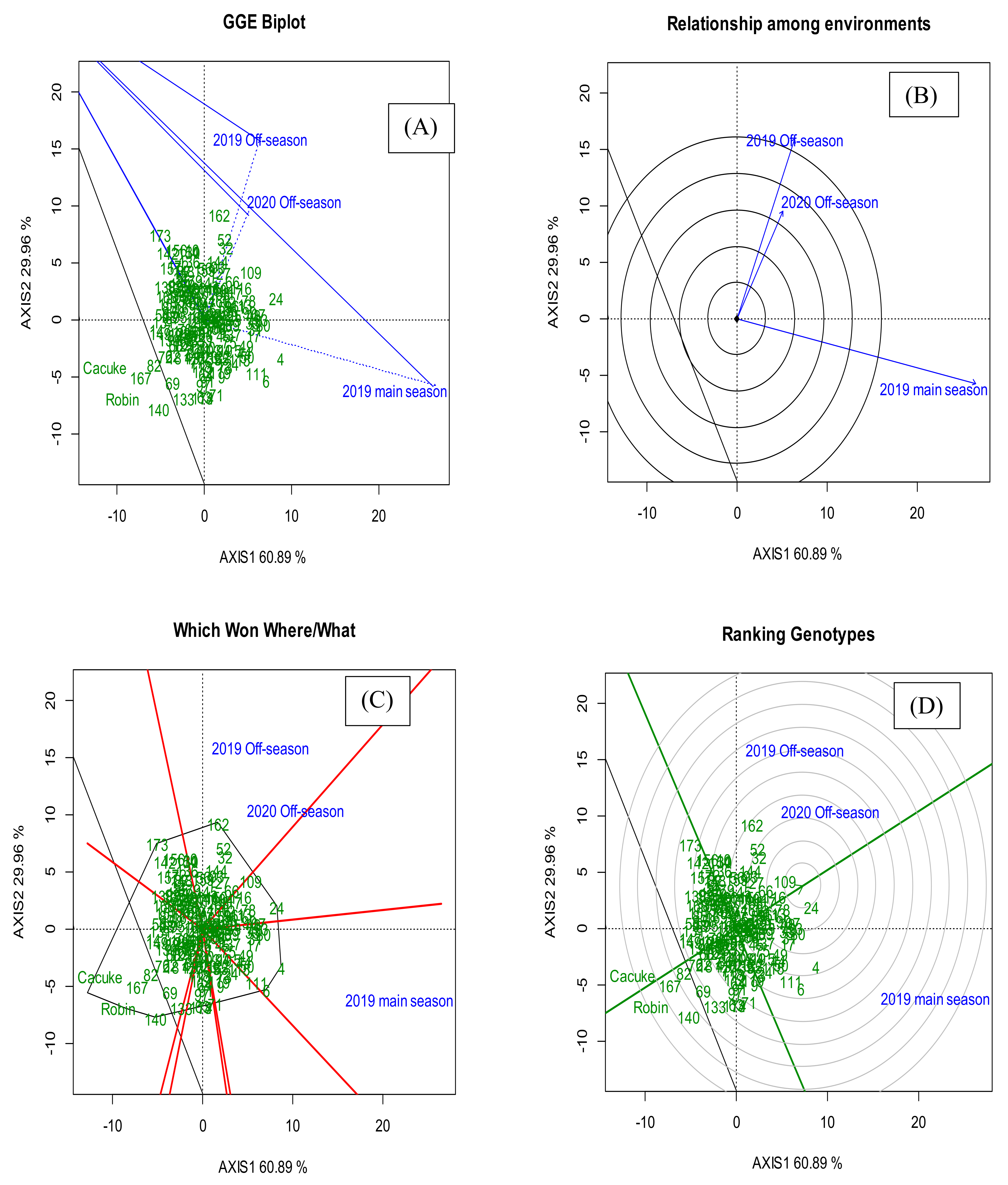
3.3. The GGE Biplot Analysis

The partitioning of genotype and genotype × environment interaction through the GGE biplot showed that 90.85% of variation in GY was attributable to the genotype and genotype × environment interaction effects as indicated by the estimates from two principal analyses. The first principal component (PC1) contributed 60.89% whereas the second principal component (PC2) contributed 29.96% to the total variation in GY (Figure 1A). The GGE biplot indicated that OS 2019 and OS 2020 were highly correlated and formed the first mega environment. However, the mean GY between the two seasons significantly differed. On the other hand, MS 2019 formed the second mega environment with higher mean GY than OS 2019 and OS 2020 (Figure 1B). The polygon view on the GGE biplot was used to choose the ideal genotypes in each environment. Genotype KSRON 162, KSRON 52 and KSRON 32 had the best GY in both OS 2019 and OS 2020 whereas genotype KSRON 4, KSRON 6 and KSRON 111 had the best GY in MS 2019 (Figure 1C). Genotypes KSRON 24, KSRON 109 and KSRON 16 were ranked the best performing genotypes in GY across the seasons whereas Cacuke, Robin, KSRON 167 and KSRON 140 had the lowest GY across the seasons. (Figure 1D,

Table 5. Final disease severity, stem rust and yellow response and area under disease progress curve of the best high yielding KSRON genotypes along with susceptible checks.

		Best Performing Genotypes in Both MS 2019 and OS 2020
		Stem Rust Severity and Response						Yellow Rust Severity and Response
Genotype	Rank	2019 OS	2019 MS	2020 OS	Mean FDS + se	Response	AUDPC_Sr	2019 OS	2019 MS	2020 OS	Mean FDS + se	Response	AUDPC_Yr	GY (t ha−1)
KSRON 32	3	60.00	46.67	3.33	46.67 ± 1.94	S	503.61	0	3.33	5.33	2.89 ± 2.09	M	37.72	8.08
KSRON 52	2	13.33	13.33	5.00	10.57 ± 1.80	M	99.00	3.33	6.67	8.33	6.11 ± 1.97	M	57.17	8.26
KSRON 162	1	30.00	28.33	13.33	23.89 ± 2.33	MS	212.33	13.33	16.67	30.00	20.00 ± 1.85	M	187.06	8.50
Best Performing Genotypes Across the Seasons
KSRON 4	2	30.00	23.33	15.00	22.78 ± 1.90	MS	194.39	0.33	11.67	11.67	7.89 ± 2.84	MS	73.89	8.74
KSRON 24	1	26.67	23.33	10.00	20.00 ± 2.17	M	214.39	0.33	0.33	3.67	1.44 ± 1.72	MR	6.61	9.27
KSRON 52	6	13.33	13.22	5.00	10.56 ± 1.80	M	99.00	3.33	6.67	8.33	6.11 ± 1.97	M	57.17	8.26
KSRON 53	8	21.67	8.33	5.00	11.67 ± 3.27	MR	127.89	0.33	6.67	10.00	5.67 ± 2.16	M	45.11	8.24
KSRON 78	7	16.67	6.67	5.00	9.44 ± 1.90	RMR	100.00	5.33	5.33	20.00	10.22 ± 2.50	M	107.72	8.25
KSRON 80	5	20.00	18.33	8.33	15.56 ± 2.32	M	144.44	0.00	3.33	5.00	2.78 ± 1.58	M	18.67	8.43
KSRON 99	9	26.67	30.00	5.00	20.56 ± 3.09	M	206.67	0.00	2.00	11.67	4.56 ± 2.94	M	45.11	8.21
KSRON 107	10	30.00	30.00	11.67	23.89 ± 239	MSS	208.44	1.67	5.00	8.33	5.00 ± 1.94	M	43.17	8.18
KSRON 109	3	43.33	43.33	11.67	32.78 ± 3.00	MSS	329.17	0.00	0.33	10.00	4.44 ± 2.50	MR	38.89	8.63
KSRON 162	4	30.00	28.33	13.33	23.89 ± 2.33	M	212.33	13.33	16.67	30.00	20.00 ± 1.85	M	187.06	8.5
* Cacuke	175	100.00	73.33	100.00	91.11 ± 1.92	S	1156.11	8.67	30.00	33.33	24.00 ± 2.54	M	282.72	1.76
* Robin	174	100.00	100.00	90.00	96.67 ± 1.02	S	1265.00	6.67	5.00	13.00	8.22 ± 1.90	M	91.39	2.82
Tukey MSD0.05					18.47		206.43				7.96		71.05	3.11

OS = offseason, MS = main season, FDS = final disease severity, se = standard error, Sr = stem rust, Yr = yellow rust, AUDPC_Sr and AUDPC_Yr = area under disease progress curve for stem rust and yellow rust, GY = grain yield, * = susceptible checks. MSD = minimum significance difference. Disease severity was assessed using 0–100% modified Cobb scale (Peterson, 1948) following host response to stem rust where R—resistant, RMR—resistant to moderately resistant, MR—moderately resistant, M—moderately resistant to moderately susceptible, MS—moderately susceptible, MSS—moderately susceptible and S—susceptible.

). The genotypic variability in mean GY, SR and YR severities and response and area under disease progress curve for SR and YR is presented in Supplementary Table S2.

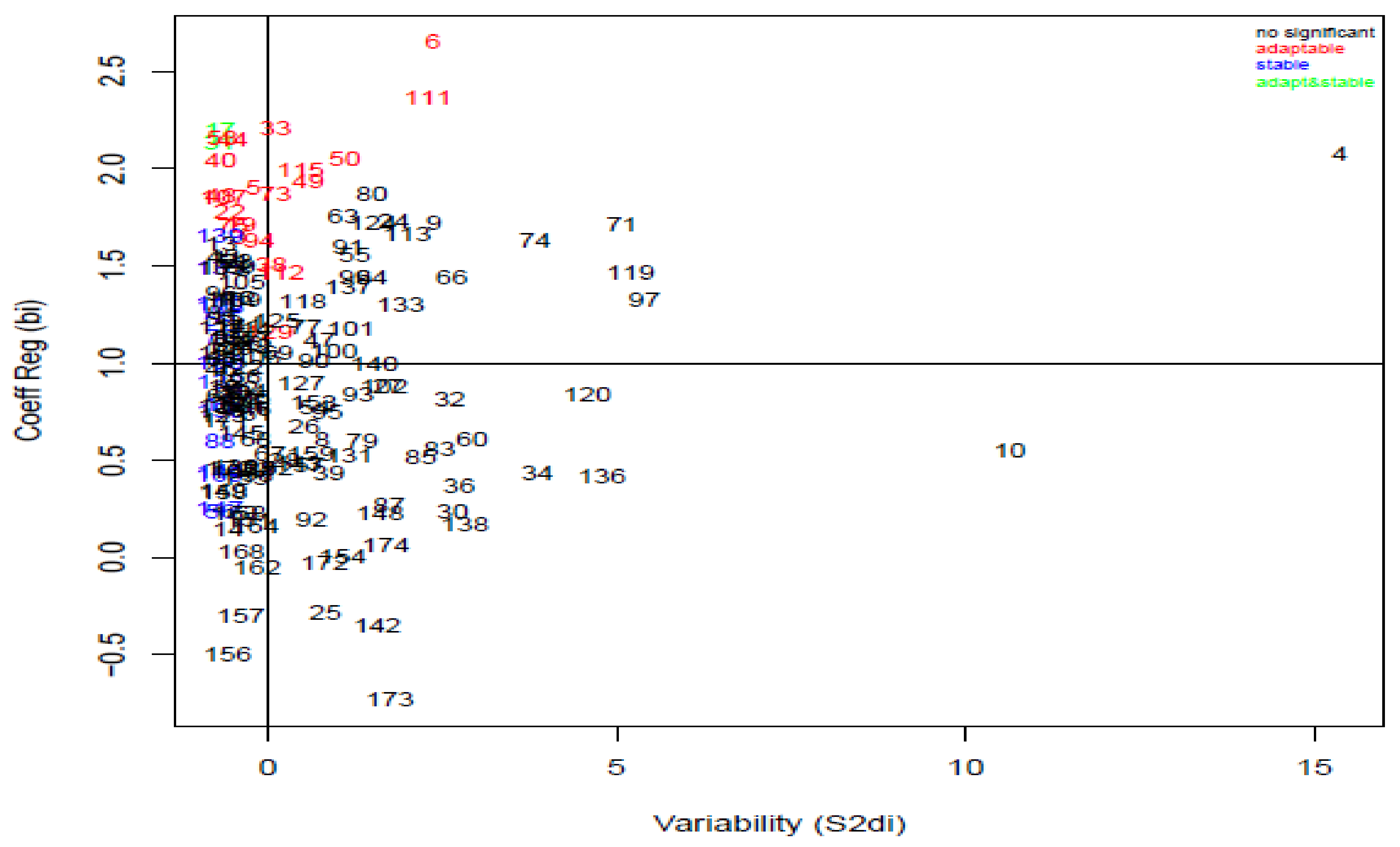
3.4. Stability Analysis

The regression coefficient ($b_i$) and deviation from the regression $S^2{d}_i$ values ranged from −0.73 to 2.65 and −0.70 to 15.37, respectively (Figure 2). The analysis identified stable genotypes, KSRON 108, KSRON 110, KSRON 132, 135, KSRON 139, KSRON 144, KSRON 147, KSRON 150, KSRON 16, KSRON 160, KSRON 169, KSRON 17, KSRON 2, KSRON 31, KSRON 56, KSRON 59, KSRON 76 and KSRON 88. Genotype KSRON 108 ($b_i$ = 1.29,$S^2{d}_i$ = −0.69, R² = 0.99) was the most stable. Genotypes KSRON 107, KSRON 111, KSRON 112, KSRON 115, KSRON 129, KSRON 17, KSRON 19, KSRON 22, KSRON 3, KSRON 31, KSRON 33, KSRON 38, KSRON 40, KSRON 44, KSRON 48, KSRON 49, KSRON 5, KSRON 50, KSRON 53, KSRON 6, KSRON 73, KSRON 75 and KSRON 95 were adaptable. Genotype KSRON 107 was the most adaptable whereas KSRON 17 and KSRON 31 were adaptable and stable.

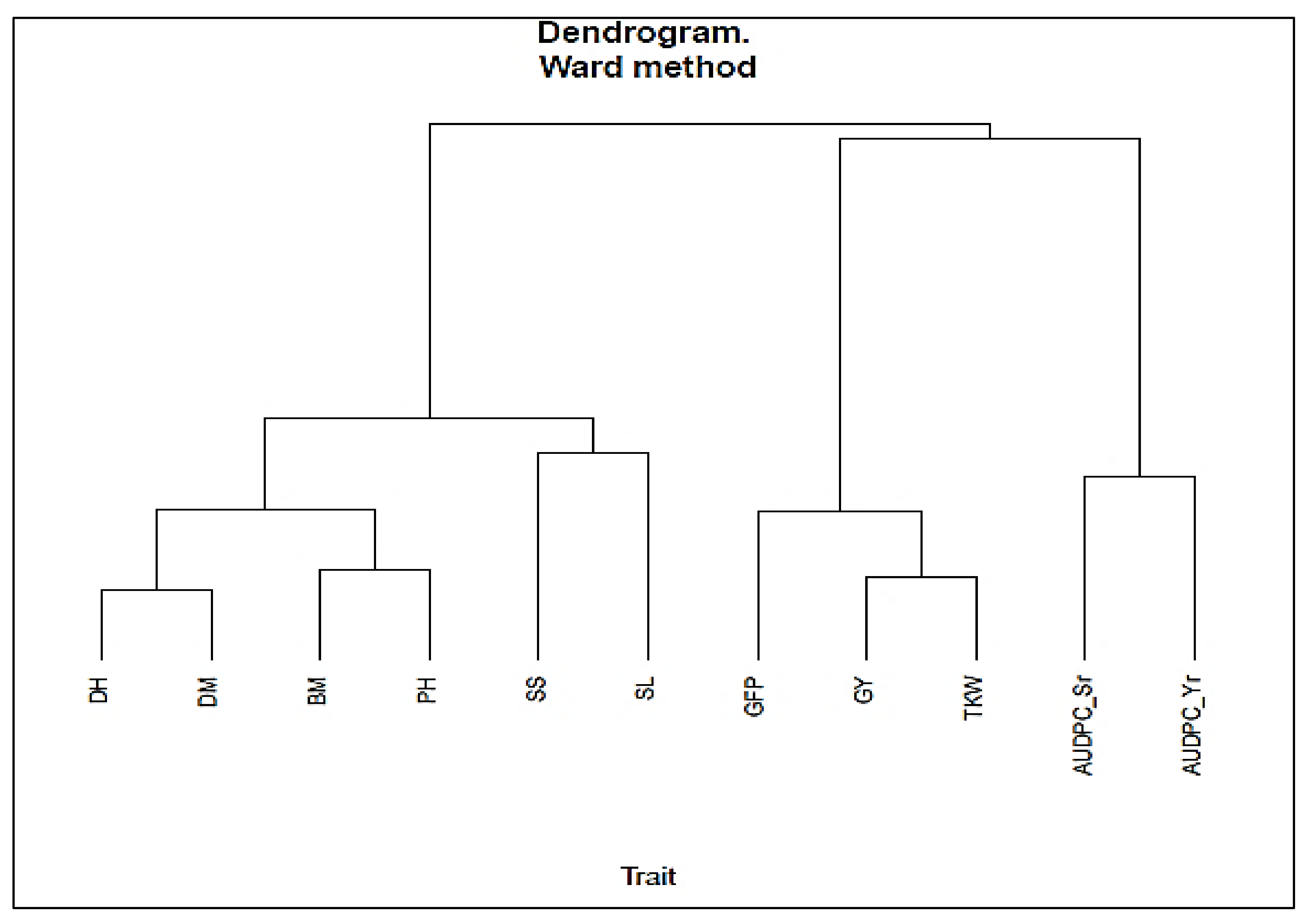
3.5. Phenotypic and Genotypic Correlation and Trait Cluster Analysis

The AUDPC_Sr had negative significant effects on GFP (r_g = −0.33 ***, r_p = −0.25 ***), BM (r_g = −0.52 ***, r_p = −0.38 ***), GY (r_g = −0.53 ***, r = −0.38 ***), TKW (r_g = −0.51 ***, r_p = −0.46 ***), DH (r_g = −0.21 ***, r_p = −0.20 **), DM (r_g = −0.52 ***, r = −0.42 ***) and SS (r_g = −0.23 **, r_p = −0.16 *) at both the genetic and the phenotypic level. The AUDPC_Yr had a negative significant correlation with GY (r_g = −0.28 ***, r_p = −0.19 *), DH (r_g = −0.16 *, r_p = −0.16 *), BM (r_g = −0.38 ***, r_p = −0.28 ***) and SS (r_g = −0.29 ***, r_p = −0.19 *) at the genetic and the phenotypic level. However, AUDPC_Yr showed a negative significant relationship with TKW (r_g = −0.15 *) at the genetic level only. Further, AUDPC_Yr had a positive significant genetic and phenotypic correlation with AUDPC_Sr (r_g = 0.22 **, r_p = 0.16 *) (

Table 6. Genetic (G) and phenotypic (P) correlation coefficients (r), area under disease progress curve for stem rust and yellow rust and yield and yield related components of KSRON wheat genotypes.

Traits		AUDPC_Sr	AUDPC_Yr	DH	BM	GY	TKW	DM	GFP
AUDPC_Yr	G P	0.22 ** 0.16 *
DH	G P	−0.21 ** −0.20 **	−0.16 * −0.16 *
BM	G P	−0.52 *** −0.38 ***	−0.38 *** −0.28 ***	0.51 *** 0.35 ***
GY	G P	−0.53 *** −0.38 ***	−0.28 *** −0.19 *	−0.13 −0.09	0.55 *** 0.45 ***
TKW	G P	−0.51 *** −0.46 ***	−0.15 * −0.12	−0.27 *** −0.24 **	0.37 *** 0.30 ***	0.65 *** 0.49 ***
DM	G P	−0.52 *** −0.42 ***	−0.09 −0.11	0.70 *** 0.56 ***	0.68 *** 0.52 ***	0.16 * 0.13	0.13 0.14
GFP	G P	−0.33 *** −0.25 **	0.11 0.06	−0.53 *** −0.45 ***	0.10 0.18 *	0.35 *** 0.23 **	0.52 *** 0.40 ***	0.22 ** 0.48 ***
SS	G P	−0.23 ** −0.16 *	−0.29 *** −0.19 *	0.28 *** 0.19 *	0.32 *** 0.23 **	0.25 *** 0.20 **	−0.24 ** −0.15	0.26 *** 0.11	−0.88 −0.08

*, **, ***, significant at p ≤ 0.05, p ≤ 0.01, p ≤ 0.001, respectively, SL = spike length, DH = days to heading, DM = days to maturity, GFP = grain filling period, GY = grain yield, TKW = 1000-kernel weight, BM = biomass, AUDPC_Sr and AUDPC_Yr = area under disease progress curve for stem rust and yellow rust.

).

The TKW (r_g = 0.65 ***, r_p = 0.49 ***), GFP (r_g = 0.35 ***, r_p = 0.23 **), BM (r_g = 0.55 ***, r_p = −0.45 ***) and SS (r_g = 0.25 ***, r_p = 0.20 **) had significant effects on GY at both the genetic and phenotypic levels. Moreover, TKW had a positive significant correlation with BM (r_g = 0.37 ***, r_p = 0.30 ***) and GFP (r_g = 0.52 ***, r_p = 0.40 ***). In addition, genotypes with high TKW took a fewer number of days to head (r_g = −0.27 ***, r_p = −0.24 **) and had few SS (r_g = −0.24 **).

From the cluster analysis, DH, DM, PH, BM, SS and SL were grouped in cluster I. GFP, GY and TKW were grouped in cluster II, while stem rust and yellow rust severity were grouped in cluster III depicting relatedness within clusters. Moreover, DH and DM, PH and BM, SL and SS, seemed to be highly related, respectively (Figure 3).

3.6. Stepwise Regression Analysis

A stepwise regression analysis forward selection was used to determine the effects of SR and YR on TKW, GY and BM of the genotypes. SR was the main cause of reduction in GY, TKW and BM. SR contributed 22% reduction in TKW, 14% reduction in GY and 14% reduction in BM over the seasons. YR resulted in 2% reduction in GY and 4% reduction in BM over the seasons (

Table 7. Stepwise multiple regression analysis for stem rust and yellow rust severity on 1000-kernel weight, grain yield and biomass of KSRON wheat genotypes evaluated over 3 seasons.

Dependable Variable	Independent Variable	Intercept	Parameter Estimate	Standard Error	Partial R2	Model R2	C(P)
TKW	AUDPC_Sr	32.31	−0.01029	0.00148	0.22	0.22	1.44
GY	AUDPC_Sr	7.26	−0.00238	0.00047	0.14	0.14	4.18
	AUDPC_Yr		−0.00260	0.00146	0.02	0.16	3.00
BM	AUDPC_Sr	43.26	−0.01227	0.00258	0.14	0.14	10.25
	AUDPC_Yr		−0.02422	0.00796	0.04	0.18	3.00

R² = coefficient of determination, C(P) = Mallow’s complexity parameter, GY = grain yield, TKW = 1000-kernel weight, BM = biomass, AUDPC_Sr and AUDPC_Yr = area under disease progress curve for stem rust and yellow rust.

). YR did not have significant reduction in TKW and thus it was not fit to be added in the model.

4. Discussion

The genotypic effect was significant for PH, DH, DM, GFP, GY, TKW, AUDPC_Sr and AUDPC_Yr. This indicated the existence of genetic variation for these traits within the genotypes [37]. Season × genotype interaction was significant, proving the influence of seasonal changes on the performance of the genotypes. This influence could be due to non-additivity of the seasonal effects on the expression of polygenic traits [38]. A breeder should deconstruct the observable variation and partition it into heritable and non-heritable variations [39]. Traits with high heritability included DH, TKW, DM, PH, and SL. Number of seeds per spike (SS), GY and BM had moderate broad-sense heritability, probably because they are under the control of additive genes and hence influenced by the environment [40,41]. GY had the least heritability estimates because it is a complex trait controlled by multiple genes and influenced by the interaction of the genotypic expression of yield components and the environmental variables. The heterogeneity of environmental conditions over time tends to mask the genetic potency of traits determined by multiple genes [8,9].

The AMMI analysis indicated that seasons contributed 48.20% variation in GY which was in consistence with significant differences in mean seasonal GY among the genotypes. This explained why MS 2019 had the highest mean GY than OS 2019 and OS 2020. The GGE biplot analysis indicated that the OS 2019 and OS 2020 were highly correlated despite their yield performance being significantly different. This also showed that KSRON genotypes were sensitive to environmental change impacting on their production stability which might be a challenge in crop improvement. However, MS 2019 had the highest mean GY than OS 2019 and OS 2020 since it is the main wheat growing season in Kenya. These results are in agreement with Sgrò and Hoffmann [42] who reported that, evaluating genotypes in similar or interrelated environments might synchronize their performance resulting in a strong genetic correlation.

KSRON 162, KSRON 52 and KSRON 32 were the best performing genotypes in the OFS 2019 and OFS 2020, while KSRON 4, KSRON 6 and KSRON 111 were the best genotypes in MS 2019 exhibiting agronomic (dynamic) stability due to cross over interaction. Becker and Leon [43] and Yan and Kung [44] reported that a good genotype must be widely adaptable, stable and have a high mean grain yield. The combination of high yielding, yield stability and stem rust resistance are a desired trait combination for wheat improvement in Kenya. Genotypes, KSRON 2, KSRON 108 and KSRON 144 showed biological (static) stability and thus were less responsive to seasonal variation displaying non-crossover interaction. These genotypes were also high yielding, resistant to stem rust and yellow rust over the seasons. This is in line with Powell et al. [45] and Sharma and Duveiller [46] who reported the possibility of the selection of wheat genotypes with a combination of high yielding, disease resistant, early maturing and high kernel quality traits. In developing countries and global scale genotypes possessing resistance to diseases coupled with high yielding traits are environmentally friendly and significant in promoting food and nutrition security.

The stepwise regression analysis showed that stem rust and yellow rust significantly reduced GY, TKW and BM over the seasons. Post-anthesis biotic stress limits the full potential of wheat cultivars in the expression of these traits by reducing the number of fertile florets, shortening the grain filling period which also translates to a reduced assimilate accumulation and grain weight. Asmmawy et al. [47] and Macharia and Wanyera [5] demonstrated a negative linear relationship between disease infection, low grain yield and 1000-kernel weight. In Ethiopia, Olivera et al. [48] reported more than 90% yield losses on wheat cultivar Digalu caused by SR race TKTTF in 2013/2014 cropping season. These reports are in line with the results from this study where AUDPC_Sr negatively correlated with GY, TKW, BM and GFP. The results suggested that, GY, TKW and BM reduced with the increase in stem rust severity due to the negative influence of disease to plant metabolic process [49,50].

Genotype KSRON 167 was resistant to both stem rust and yellow rust and recorded the third lowest yield. This might be due to yield penalty linked to the response and expression of resistance genes in preventing rust infection [51,52]. Plants direct most of their accumulated assimilates towards the releasing of pathogenesis related proteins in terms of resistance genes to fight invading pathogens instead of kernel nourishment and development [52]. Further, yield reduction can be as a result of linkage drag associated with resistance gene (s) from alien relatives. Dundas et al. [53] and Knott [54] reported a 9% yield penalty associated with Sr26 stem rust resistance gene introgressed in wheat from Agropyron elonagatum (syn. Thinopyrum ponticum). However, genotypes KSRON 32, KSRON 120, KSRON 135 and KSRON 159, had high AUDPC_Sr with high grain yield. Similarly, KSRON 107 and KSRON 109, despite exhibiting slow rusting nature, expressed an MSS reaction to stem rust pathogen. This might be attributed to the presence of high yielding and disease resistance gene(s) being in the repulsion phase rather than coupling [55].

In this study, GY correlated with TKW, GFP, DH, DM, SS and BM. Late maturing plants tended to be taller with high BM and a longer grain filling period than early maturing types. Molero and Reynolds [56] suggested that during the grain filling period, the grain receives assimilates from the pre-anthesis stem reserves, post anthesis leaf photosynthesis and spike photosynthesis which translates high yield and 1000-kernel weight. Further, Monpara [57] reported that the grain filling period can be used to quantify the grain yield, harvest index and kernel weight in bread wheat. These reports are in line with the correlation and cluster analysis which showed that, GFP, TKW and GY are highly related.

5. Conclusions

Seasons, genotype and season × genotype interaction contributed to variation in GY and yield related traits. AMMI and GGE analyses elucidated the contribution of the main effects and their interaction to traits and helped to visualize the stability of genotypes across environments. GFP, DM and BM can be used as a basis for selection for high GY and TKW. Genotypes KSRON 13, KSRON 31, KSRON 40, KSRON 52, KSRON 53, KSRON 78, KSRON 80 and KSRON 144 were identified as the entries with high GY, TKW and high resistance to SR and YR.

References

1. Afzal, F.; Chaudhari, S.K.; Gul, A.; Farooq, A.; Ali, H.; Nisar, S.; Sarfraz, B.; Shehzadi, K.J.; Mujeeb-Kazi, A. Bread wheat (Triticum aestivum L.) under biotic and abiotic stresses: An overview. In Crop Production and Global Environmental Issues. Plant Pathology, 5th ed.; Agrios, G.N., Ed.; Elsevier Academic Press: Cambridge, MA, USA, 2015; pp. 293–317. [Google Scholar]
2. Figueroa, M.; Hammond-Kosack, K.E.; Solomon, P.S. A review of wheat diseases—A field perspective. Mol. Plant Pathol. 2018, 19, 1523–1536. [Google Scholar] [CrossRef] [PubMed]
3. Kogo, B.K.; Kumar, L.; Koech, R. Climate change and variability in Kenya: A review of impacts on agriculture and food security. Environ. Dev. Sustain. 2021, 23, 23–43. [Google Scholar] [CrossRef]
4. CIMMYT. Sounding the Alarm on Global Stem Rust: An Assessment of Race Ug99 in Kenya and Ethiopia and the Potential for Impact in Neighboring Countries and Beyond; CIMMYT: Mexico City, Mexico, 2005. [Google Scholar]
5. Macharia, J.K.; Wanyera, R. Effect of stem rust race Ug99 on grain yield and yield components of wheat cultivars in Kenya. J. Agric. Sci. Technol. A 2012, 2, 423. [Google Scholar]
6. Singh, R.P.; Hodson, D.P.; Huerta-Espino, J.; Jin, Y.; Bhavani, S.; Njau, P.; Herrera-Foessel, S.; Singh, P.K.; Singh, S.; Govindan, V. The emergence of Ug99 races of the stem rust fungus is a threat to world wheat production. Annu. Rev. Phytopathol. 2011, 49, 465–481. [Google Scholar] [CrossRef] [PubMed] [Green Version]
7. Pennacchi, J.P.; Carmo-Silva, E.; Andralojc, P.J.; Lawson, T.; Allen, A.M.; Raines, C.A.; Parry, M. Stability of wheat grain yields over three field seasons in the UK. Food Energy Secur. 2019, 8, e00147. [Google Scholar] [CrossRef] [Green Version]
8. Sial, M.A.; Arain, M.A.; Naqvi, M.H.; Soomro, A.M.; Laghari, S.; Nizamani, N.A.; Ali, A. Seasonal effects and genotypic responses for grain yield in semi-dwarf wheat. Asian J. Plant Sci. 2003, 2, 1097–1101. [Google Scholar] [CrossRef]
9. Subira, J.; Álvaro, F.; del Moral, L.F.G.; Royo, C. Breeding effects on the cultivar×environment interaction of durum wheat yield. Eur. J. Agron. 2015, 68, 78–88. [Google Scholar] [CrossRef] [Green Version]
10. Braun, H.J.; Atlin, G.; Payne, T. Multi-location testing as a tool to identify plant response to global climate change. Clim. Chang. Crop Prod. 2010, 1, 115–138. [Google Scholar] [CrossRef]
11. Fischer, R.A.; Byerlee, D.; Edmeades, G. Crop Yields and Global Food Security; ACIAR: Canberra, ACT, Australia, 2014; pp. 8–11. [Google Scholar]
12. Baloch, M.J.; Baloch, E.; Jatoi, W.A.; Veesar, N.F. Correlations and heritability estimates of yield and yield attributing traits in wheat (Triticum aestivum L.). Pak. J. Agric. 2013, 29, 96–105. [Google Scholar]
13. Mansouri, A.; Oudjehih, B.; Benbelkacem, A.; Fellahi, Z.E.A.; Bouzerzour, H. Variation and Relationships among Agronomic Traits in Durum Wheat (Triticum turgidum (L.) Thell. ssp. turgidumconv. Durum (Desf.) MacKey) under South Mediterranean Growth Conditions: Stepwise and Path Analyses. Int. J. Agron. 2018, 2018, 1–11. [Google Scholar] [CrossRef]
14. Falconer, D.S.; Mackay, T.F.C. Introduction to Quantitative Genetics; Longman: London, UK, 1996. [Google Scholar]
15. Daday, H.; Binet, F.E.; Grassia, A.; Peak, J.W. The effect of environment on heritability and predicted selection response in Medicago sativa. Heredity 1973, 31, 293–308. [Google Scholar] [CrossRef] [Green Version]
16. Vargas, M.; Combs, E.; Alvarado, G.; Atlin, G.; Mathews, K.; Crossa, J. META: A suite of SAS programs to analyze multien-vironment breeding trials. Agron. J. 2013, 105, 11–19. [Google Scholar] [CrossRef] [Green Version]
17. Cox, T.S.; Shroyer, J.P.; Ben-Hui, L.; Sears, R.G.; Martin, T.J. Genetic improvement in agronomic traits of hard red winter wheat cultivars 1919 to 1987. Crop Sci. 1988, 28, 756–760. [Google Scholar] [CrossRef]
18. Finlay, K.; Wilkinson, G. The analysis of adaptation in a plant-breeding programme. Aust. J. Agric. Res. 1963, 14, 742–754. [Google Scholar] [CrossRef] [Green Version]
19. Eberhart, S.A.; Russell, W.A. Stability parameters for comparing varieties. Crop Sci. 1966, 6, 36–40. [Google Scholar] [CrossRef] [Green Version]
20. Perkins, J.M.; Jinks, J.L. Environmental and genotype-environmental components of variability III. Multiple lines and crosses. Heredity 1968, 23, 339–356. [Google Scholar] [CrossRef] [Green Version]
21. Shukla, G.K. Some statistical aspects of partitioning genotype-environmental components of variability. Heredity 1972, 29, 237–245. [Google Scholar] [CrossRef] [PubMed]
22. Allard, R.W.; Bradshaw, A.D. Implications of genotype-environmental interactions in applied plant breeding 1. Crop Sci. 1964, 4, 503–508. [Google Scholar] [CrossRef] [Green Version]
23. Bassi, F.M.; Sanchez-Garcia, M. Adaptation and stability analysis of ICARDA durum wheat elites across 18 countries. Crop Sci. 2017, 57, 2419–2430. [Google Scholar] [CrossRef]
24. Singh, C.; Gupta, A.; Gupta, V.; Kumar, P.; Sendhil, R.; Tyagi, B.; Singh, G.; Chatrath, R.; Singh, G. Genotype x environment interaction analysis of multi-environment wheat trials in India using AMMI and GGE biplot models. Crop Breed. Appl. Biotechnol. 2019, 19, 309–318. [Google Scholar] [CrossRef]
25. Kun, S.; Lijuan, Y.; Xiaohang, L.; Yang, G.; Zhikai, J.; Aiwang, D. Grain quality variations from year to year among the Chinese genotypes. Cereal Res. Commun. 2020, 48, 499–505. [Google Scholar] [CrossRef]
26. Jaetzold, R.; Hornetz, B.; Shisanya, C.A.; Schmidt, H. Farm Management Handbook of Kenya Vol I–IV (Western Central Eastern Nyanza Southern Rift Valley Northern Rift Valley Coast); Government Printers: Nairobi, Kenya, 2012. [Google Scholar]
27. Zadoks, J.C.; Chang, T.T.; Konzak, C.F. A decimal code for the growth stages of cereals. Weed Res. 1974, 14, 415–421. [Google Scholar] [CrossRef]
28. Peterson, R.F.; Campbell, A.B.; Hannah, A.E. A diagrammatic scale for estimating rust intensity on leaves and stems of cereals. Can. J. Res. 1948, 26c, 496–500. [Google Scholar] [CrossRef]
29. AACC (American Association of Cereal Chemists). International Approved Methods of the American Association of Cereal Chemist, 10th ed.; AACC (American Association of Cereal Chemists): St. Paul, MN, USA, 2000; Volume 1, Method 1200.56. [Google Scholar]
30. CIMMYT. A Programme for Calculation of AUDPC. Mexico D. F a Software Package; CIMMYT: Mexico City, Mexico, 2008. [Google Scholar]
31. SAS Institute. SAS Software, User Guide: Statistics; SAS Institute: Cary, NC, USA, 2001. [Google Scholar]
32. Tukey, J.W. Comparing individual means in the analysis of variance. Biometrics 1949, 5, 99. [Google Scholar] [CrossRef]
33. Pacheco, A.; Vargas, M.; Alvarado, G.; Rodríguez, F.; Crossa, J.; Burgueño, J. GEA-R (Genotype x Environment Analysis with R for Windows) Version 4.1; CIMMYT Research Data & Software Repository Network, CIMMYT: El Batan, Mexico, 2015; Volume 16, Available online: https://hdl.handle.net/11529/10203 (accessed on 1 September 2021).
34. Hill, W.G.; Singh, R.K.; Chaudhary, B.D. Biometrical Methods in Quantitative Genetic Analysis; Kalyani: Ludhiana, India, 1977. [Google Scholar]
35. Miller, P.A.; Williams, J.C.J.; Robinson, H.F.; Comstock, R.E. Estimates of genotypic and environmental variances and co-variances in upland cotton and their implications in selection 1. Agron. J. 1958, 50, 126–131. [Google Scholar] [CrossRef]
36. Alvarado, G.; López, M.; Vargas, M.; Pacheco, A.; Rodriguez, F.; Burgueno, J.; Crossa, J. META-R (Multi-Environment Trail Analysis with R for Windows) Version 5; International Maize and Wheat Improvement Center: Mexico City, Mexico, 2015. [Google Scholar]
37. Rehman, S.U.; Abid, M.A.; Bilal, M.; Ashraf, J.; Liaqat, S.; Ahmed, R.I.; Qanmber, G. Genotype by trait analysis and estimates of heritability of wheat (Triticum aestivum L.) under drought and control conditions. Basic Res. J. Agric. Sci. Rev. 2015, 4, 127–134. [Google Scholar]
38. Weinig, C.; Schmitt, J. Environmental effects on the expression of quantitative trait loci and implications for phenotypic evo-lution. Bioscience 2004, 54, 627–635. [Google Scholar] [CrossRef] [Green Version]
39. Balkan, A. Genetic variability, heritability and genetic advance for yield and quality traits in M2-4 generations of bread wheat (Triticum aestivum L.) genotypes. Turk. J. Field Crop 2018, 23, 173–179. [Google Scholar] [CrossRef]
40. De Vita, P.; Mastrangelo, A.; Matteu, L.; Mazzucotelli, E.; Virzì, N.; Palumbo, M.; Storto, M.L.; Rizza, F.; Cattivelli, L. Genetic improvement effects on yield stability in durum wheat genotypes grown in Italy. Field Crop Res. 2010, 119, 68–77. [Google Scholar] [CrossRef]
41. Kumar, N.; Markar, S.; Kumar, V. Studies on heritability and genetic advance estimates in timely sown bread wheat (Triticum aestivum L.). Biosci. Discov. 2014, 5, 64–69. [Google Scholar]
42. Sgrò, C.M.; Hoffmann, A. Genetic correlations, tradeoffs and environmental variation. Heredity 2004, 93, 241–248. [Google Scholar] [CrossRef] [Green Version]
43. Becker, H.C.; Leon, J. Stability analysis in plant breeding. Plant Breed. 1988, 101, 1–23. [Google Scholar] [CrossRef]
44. Yan, W.; Kang, M.S. GGE Biplot Analysis: A Graphical Tool For Breeders, Geneticists And Agronomists, 1st ed.; CRC Press LLC: Boca Roton, FL, USA, 2003; p. 271. [Google Scholar]
45. Powell, N.M.; Lewis, C.M.; Berry, S.T.; MacCormack, R.; Boyd, L.A. Stripe rust resistance genes in the UK winter wheat cultivar Claire. Theor. Appl. Genet. 2013, 126, 1599–1612. [Google Scholar] [CrossRef] [PubMed]
46. Sharma, R.C.; Duveiller, E. Selection index for improving Helminthosporium leaf blight resistance, maturity, and kernel weight in spring wheat. Crop Sci. 2003, 43, 2031–2036. [Google Scholar] [CrossRef]
47. Asmmawy, M.A.; El-Orabey, W.M.; Nazim, M.; Shahin, A.A. Effect of stem rust infection on grain yield and yield components of some wheat cultivars in Egypt. Int. J. Phytopathol. 2013, 2, 171–178. [Google Scholar] [CrossRef]
48. Olivera, P.; Newcomb, M.; Szabo, L.J.; Rouse, M.; Johnson, J.; Gale, S.; Luster, D.G.; Hodson, D.; Cox, J.A.; Burgin, L.; et al. Phenotypic and genotypic characterization of race TKTTF of Puccinia graminis f. sp. tritici that caused a wheat stem rust epidemic in Southern Ethiopia in 2013–2014. Phytopathology 2015, 105, 917–928. [Google Scholar] [CrossRef] [PubMed] [Green Version]
49. Abdulbagiyeva, S.; Zamanov, A.; Talai, J.; Allahverdiyev, T. Effect of rust disease on photosynthetic rate of wheat plant. J. Agric. Sci. Technol. B 2015, 5, 5. [Google Scholar] [CrossRef] [Green Version]
50. Chen, Y.E.; Cui, J.M.; Su, Y.Q.; Yuan, S.; Yuan, M.; Zhang, H.Y. Influence of stripe rust infection on the photosynthetic char-acteristics and antioxidant system of susceptible and resistant wheat cultivars at the adult plant stage. Front. Plant Sci. 2015, 6, 779. [Google Scholar] [CrossRef] [Green Version]
51. Brown, J.K.M. Yield penalties of disease resistance in crops. Curr. Opin. Plant Biol. 2002, 5, 339–344. [Google Scholar] [CrossRef]
52. Summers, R.W.; Brown, J.K.M. Constraints on breeding for disease resistance in commercially competitive wheat cultivars. Plant Pathol. 2013, 62, 115–121. [Google Scholar] [CrossRef]
53. Dundas, I.S.; Anugrahwati, D.R.; Verlin, D.C.; Park, R.F.; Bariana, H.S.; Mago, R.; Islam, A.K.M.R. New Sources of rust re-sistance from alien species: Meliorating linked defects and discovery. Aust. J. Agric. Res. 2007, 58, 545–549. [Google Scholar] [CrossRef]
54. Knott, D.R. The inheritance of rust resistance. VI. The transfer of stem rust resistance from agropyron elongatum to common wheat. Can. J. Plant Sci. 1961, 41, 109–123. [Google Scholar] [CrossRef]
55. Daspute, A.; Fakrudin, B. Identification of coupling and repulsion phase DNA marker associated with an allele of a gene conferring host plant resistance to pigeon pea sterility mosaic virus (PPSMV) in pigeon pea (Cajanus cajan L. Millsp.). Plant Pathol. J. 2015, 31, 33–40. [Google Scholar] [CrossRef] [PubMed] [Green Version]
56. Molero, G.; Reynolds, M.P. Spike photosynthesis measured at high throughput indicates genetic variation independent of flag leaf photosynthesis. Field Crop Res. 2020, 255, 107866. [Google Scholar] [CrossRef]
57. Monpara, B.A. Grain filling period as a measure of yield improvement in bread wheat. Crop Improv. 2011, 38, 1–5. [Google Scholar]
Figure 1. Genotype and genotype by environment interaction biplot (GGE) showing (A) principal component analysis (PCA) 1 (AXIS1) and principal component analysis 2 (AXIS2), (B) the relationship among environments for grain yield, (C) which, won, and where for genotypes and seasons, and (D) mean ranking over the seasons for KSRON wheat genotypes.
Agronomy 11 02394 g001
Figure 2. Yield stability among KSRON wheat genotypes plotted from Eberhart and Russell joint regression coefficients. bi = regression coefficient and S2di = deviation from regression.
Agronomy 11 02394 g002
Figure 3. Dendrogram showing relationship between yield, and yield components of KSRON genotypes. GFP = grain filling period, GY = grain yield, TKW = 1000-kernel weight, AUDPC_Sr and AUDPC_Yr = Area under disease progress curve for stem rust and yellow rust, DH = days to heading, DM = days to maturity, PH = plant height, BM = biomass, SL = spike length, SS = seed spike−1.
Agronomy 11 02394 g003