
Modelling the Interactions of Soils, Climate, and Management for Grass Production in England and Wales

 ,
,  , , , ,
Abstract
:1. Introduction
2. Methodology
2.1. Model Development and Calibration
2.1.1. Soil Nitrogen Availability
2.1.2. Thermal Time Functions for Above-Ground Partitioning
2.1.3. Composition of the Harvested Yield
2.2. Validation of LINGRA-N-Plus
2.3. Analysis of Soil and Climate Factors
3. Results
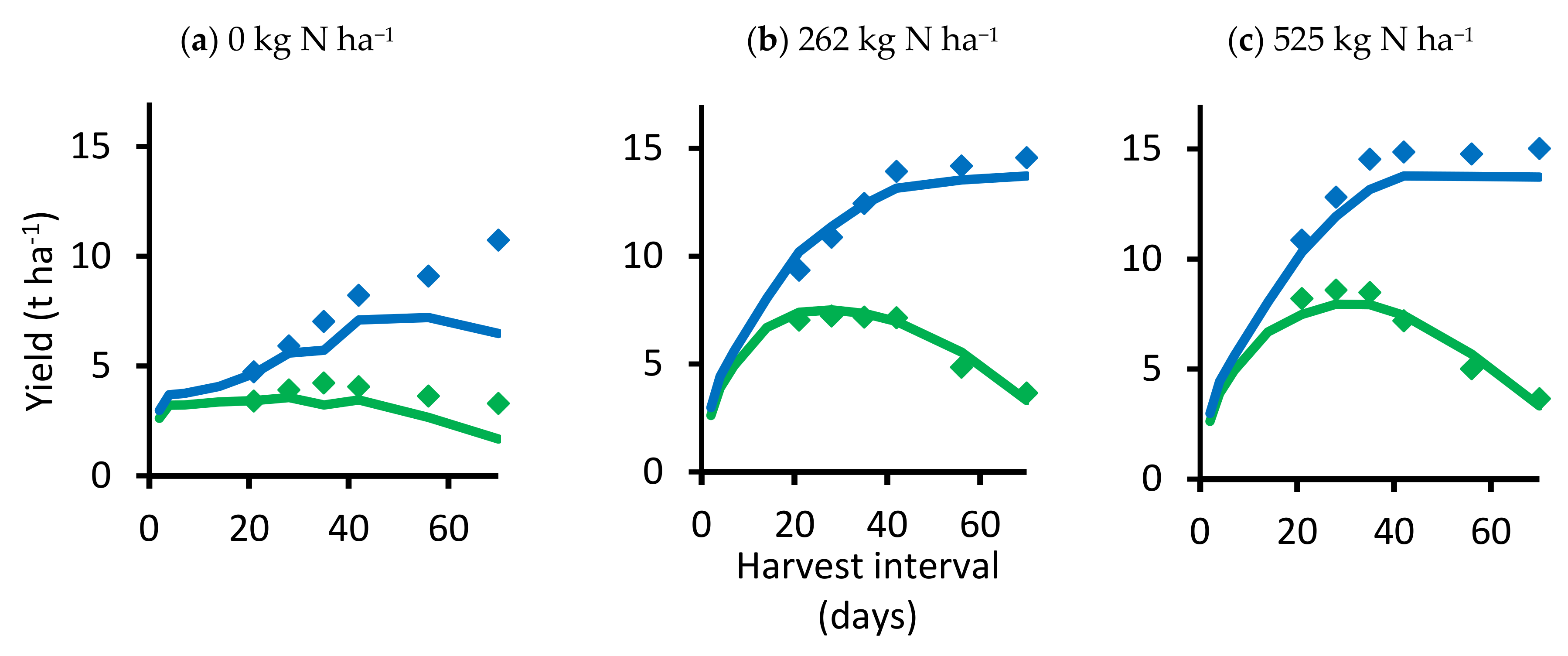
3.1. Development and Calibration of the Model
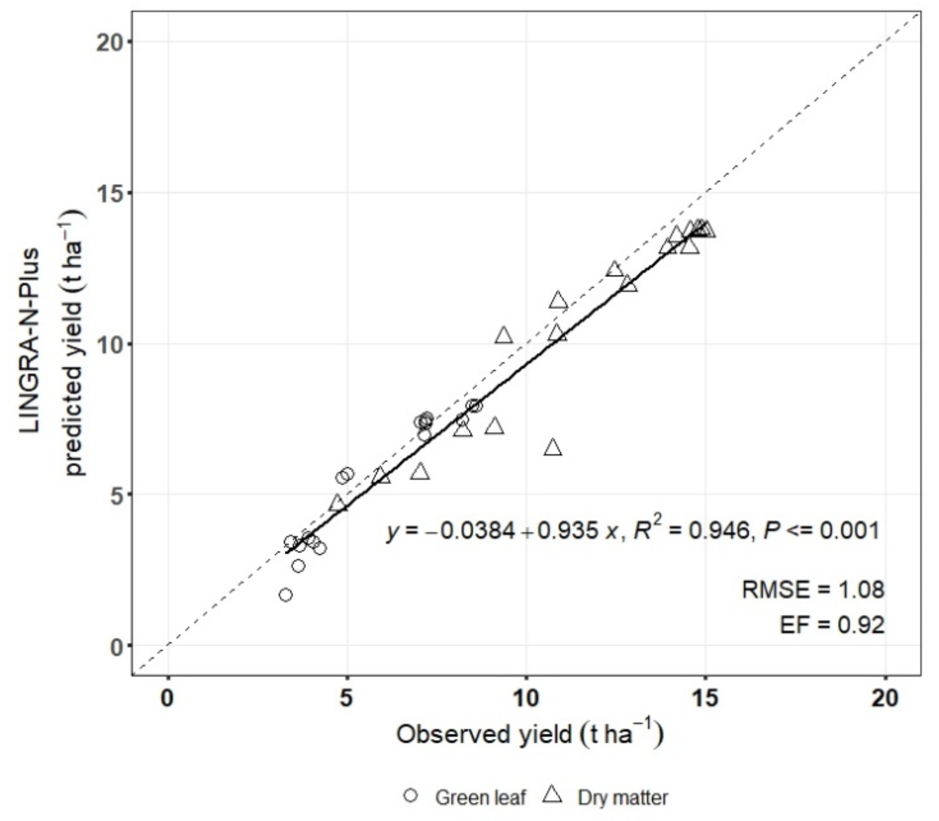
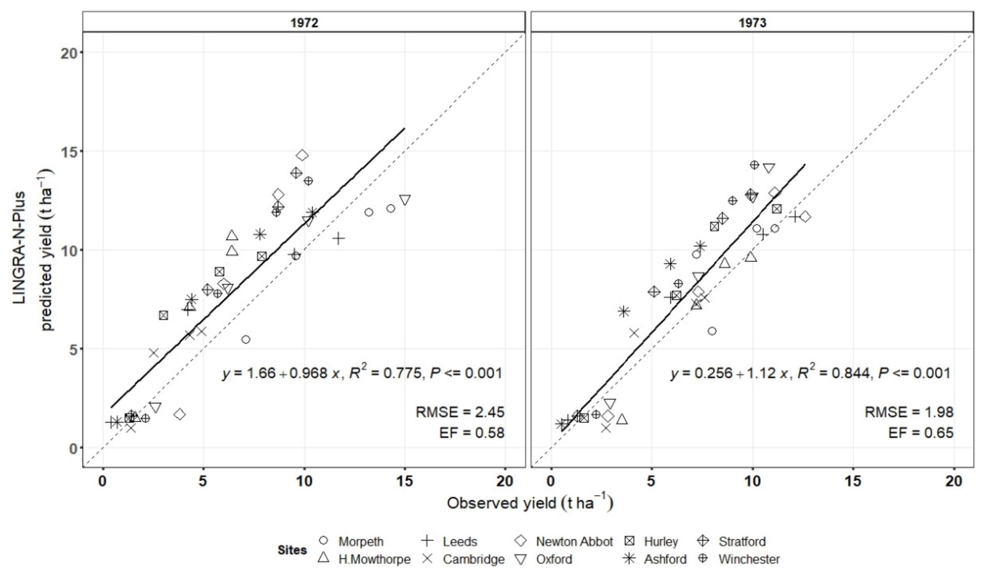
3.2. Validation of the LINGRA-N-Plus Model (Morrison Experimental Data)
3.3. Comparison of the Results from LINGRA with Those from LINGRA-N-Plus
3.4. Climate, Soil, and Nitrogen Interactions on Grass Yields
4. Discussion
4.1. Improvement and Validation of the Model
4.2. Effect of Climate, Soil, Harvest Interval and Nitrogen on Yields
4.3. Soil and Nitrogen Uptake Efficiency
5. Conclusions
Author Contributions
Funding
Institutional Review Board Statement
Informed Consent Statement
Data Availability Statement
Acknowledgments
Conflicts of Interest
Appendix A

| Harvest Interval (Weeks) | 3 | 4 | 5 | 6 | 8 | 10 |
|---|---|---|---|---|---|---|
| Number of Harvests | 10 | 8 * | 6 | 5 | 3 + | 3 |
| Date ** | ||||||
| 16 April | 1st | - | - | - | - | - |
| 23 | - | 1st | - | - | - | - |
| 30 | - | - | 1st | - | - | - |
| 07 May | 2nd | - | - | 1st | - | - |
| 21 | - | 2nd | - | - | 1st | - |
| 28 | 3rd | - | - | - | - | - |
| 04 June | - | - | 2nd | - | - | 1st |
| 18 | 4th | 3rd | - | 2nd | - | - |
| 09 July | 5th | - | 3rd | - | - | - |
| 16 | - | 4th | - | - | 2nd | - |
| 30 | 6th | - | - | 3rd | - | - |
| 13 August | - | 5th | 4th | - | - | 2nd |
| 20 | 7th | - | - | - | - | - |
| 10 September | 8th | 6th | - | 4th | 3rd | - |
| 17 | - | - | 5th | - | - | - |
| 01 October | 9th | - | - | - | - | - |
| 8 | - | 7th | - | - | - | - |
| 22 | 10th | 8th | 6th | 5th | 4th | 3rd |
| BBCH Stage | Description |
|---|---|
| 0 | Germination |
| 9 | Emergence of seedling at soil surface |
| 10–19 | Leaf development |
| 21 | Beginning of tillering; main shoot and one tiller detectable |
| 30 | Beginning of stem elongation |
| 50 | First spikelet of the inflorescence is just visible |
| 60 | Beginning of flowering |
| 65 | Full flowering; half of anthers mature |
| 90 | Grain fully ripe |
| Site | Cutting Dates | |||||
|---|---|---|---|---|---|---|
| Morpeth | 16 May | 13 Jun | 11 Jul | 8 Aug | 5 Sep | 3 Oct |
| High Mowthorpe | 14 May | 11 Jun | 9 Jul | 6 Aug | 3 Sep | 1 Oct |
| Leeds | 12 May | 9 Jun | 7 Jul | 4 Aug | 1 Sep | 29 Sep |
| Cambridge Stratford upon Avon | 10 May | 7 Jun | 5 Jul | 2 Aug | 30 Aug | 27 Sep |
| Newton Abbot | 6 May | 3 Jun | 1 Jul | 29 Jul | 26 Aug | 23 Sep |
| Oxford | 8 May | 5 Jun | 3 Jul | 31 Jul | 28 Aug | 25 Sep |
| Hurley | ||||||
| Ashford | ||||||
| Winchester | ||||||
| Application Date * | |||||||||
|---|---|---|---|---|---|---|---|---|---|
| Morpeth | High Mowthorpe | Leeds | Cambridge | Newton Abbot | Oxford | Hurley | Ashford | Stratford | Winchester |
| 29 Mar | 26 Mar | 23 Mar | 13 Mar | 01 Mar | 27 Mar | 19 Mar | 21 Mar | 05 Apr | 19 Mar |
| 17 May | 15 May | 13 May | 11 May | 07 May | 09 May | 09 May | 09 May | 11 May | 09 May |
| 14 Jun | 12 Jun | 10 Jun | 08 Jun | 04 Jun | 06 Jun | 06 Jun | 06 Jun | 08 Jun | 06 Jun |
| 12 Jul | 10 Jul | 08 Jul | 06 Jul | 02 Jul | 04 Jul | 04 Jul | 04 Jul | 06 Jul | 04 Jul |
| 09 Aug | 07 Aug | 05 Aug | 03 Aug | 30 Jul | 01 Aug | 01 Aug | 01 Aug | 03 Aug | 01 Aug |
| 06 Sep | 04 Sep | 02 Sep | 31 Aug | 27 Aug | 29 Aug | 29 Aug | 29 Aug | 31 Aug | 29 Aug |
| Site | SMFC (pF = 2.3) | SMPWP (pF = 4.2) | SMDRY (pF = 6) |
|---|---|---|---|
| (mm3 mm−3) | (mm3 mm−3) | (mm3 mm−3) | |
| Aberystwyth | 0.32 | 0.19 | 0.03 |
| Morpeth | 0.25 | 0.11 | 0.10 |
| High Mowthorpe | 0.36 | 0.18 | 0.15 |
| Leeds | 0.38 | 0.19 | 0.15 |
| Cambridge | 0.17 | 0.13 | 0.10 |
| Newton Abbot | 0.32 | 0.19 | 0.03 |
| Oxford | 0.28 | 0.10 | 0.10 |
| Hurley | 0.19 | 0.09 | 0.03 |
| Ashford | 0.32 | 0.19 | 0.03 |
| Stratford | 0.36 | 0.20 | 0.15 |
| Winchester | 0.36 | 0.20 | 0.15 |
| Nitrogen (kg N/ha) | Harvest Interval (days) | ||||||||||
|---|---|---|---|---|---|---|---|---|---|---|---|
| 2 | 4 | 7 | 14 | 21 | 28 | 35 | 42 | 56 | 70 | ||
| (a) Observed | |||||||||||
| 0 | Green leaf | 3.41 | 3.91 | 4.23 | 4.06 | 3.64 | 3.29 | ||||
| Total | 4.73 | 5.92 | 7.03 | 8.22 | 9.10 | 10.73 | |||||
| 262 | Green leaf | 7.04 | 7.23 | 7.18 | 7.15 | 4.86 | 3.66 | ||||
| Total | 9.36 | 10.88 | 12.45 | 13.93 | 14.19 | 14.57 | |||||
| 525 | Green leaf | 8.2 | 8.59 | 8.49 | 7.19 | 5.01 | 3.65 | ||||
| Total | 10.85 | 12.81 | 14.54 | 14.86 | 14.77 | 15.02 | |||||
| (b) Predicted | |||||||||||
| 0 | Green leaf | 2.62 | 3.22 | 3.23 | 3.36 | 3.42 | 3.56 | 3.23 | 3.45 | 2.66 | 1.67 |
| Total | 2.98 | 3.69 | 3.75 | 4.07 | 4.66 | 5.59 | 5.71 | 7.10 | 7.21 | 6.48 | |
| 262 | Green leaf | 2.62 | 3.89 | 4.93 | 6.69 | 7.40 | 7.51 | 7.35 | 6.98 | 5.55 | 3.32 |
| Total | 2.98 | 4.43 | 5.60 | 8.04 | 10.20 | 11.37 | 12.40 | 13.15 | 13.54 | 13.72 | |
| 525 | Green leaf | 2.62 | 3.89 | 4.93 | 6.69 | 7.48 | 7.94 | 7.92 | 7.43 | 5.68 | 3.32 |
| Total | 2.98 | 4.43 | 5.60 | 8.04 | 10.30 | 11.93 | 13.16 | 13.77 | 13.75 | 13.72 | |
| N app. (kg ha−1) | Morpeth | High Mow- thorpe | Leeds | Cambridge | Newton Abbot | Oxford | Hurley | Ashford | Stratford | Winchester | ||
|---|---|---|---|---|---|---|---|---|---|---|---|---|
| 1972 | 0 | Obs. | 7.1 | 1.6 | 0.4 | 1.4 | 3.8 | 2.6 | 1.3 | 0.7 | 1.4 | 2.1 |
| Pred. | 5.5 | 1.5 | 1.3 | 1.0 | 1.7 | 2.1 | 1.5 | 1.3 | 1.6 | 1.5 | ||
| 150 | Obs. | 9.6 | 4.3 | 4.2 | 2.5 | 6.0 | 6.2 | 3.0 | 4.4 | 5.2 | 5.7 | |
| Pred. | 9.7 | 7.1 | 7.0 | 4.8 | 8.3 | 8.1 | 6.7 | 7.5 | 8.0 | 7.8 | ||
| 300 | Obs. | 13.2 | 6.4 | 9.5 | 4.3 | 8.7 | 10.2 | 5.8 | 7.8 | 8.7 | 8.6 | |
| Pred. | 11.9 | 9.9 | 9.8 | 5.7 | 12.8 | 11.5 | 8.9 | 10.8 | 12.2 | 11.9 | ||
| 450 | Obs. | 14.3 | 6.4 | 11.7 | 4.9 | 9.9 | 15.0 | 7.9 | 10.4 | 9.6 | 10.2 | |
| Pred. | 12.1 | 10.7 | 10.6 | 5.9 | 14.8 | 12.6 | 9.7 | 11.9 | 13.9 | 13.5 | ||
| 1973 | 0 | Obs. | 8.0 | 3.5 | 0.8 | 2.7 | 2.8 | 2.9 | 1.6 | 0.5 | 1.3 | 2.2 |
| Pred. | 5.9 | 1.4 | 1.4 | 1.0 | 1.6 | 2.3 | 1.5 | 1.2 | 1.6 | 1.7 | ||
| 150 | Obs. | 7.2 | 7.2 | 5.9 | 4.1 | 7.3 | 7.3 | 6.2 | 3.6 | 5.1 | 6.3 | |
| Pred. | 9.8 | 7.2 | 7.6 | 5.8 | 7.9 | 8.7 | 7.7 | 6.9 | 7.9 | 8.3 | ||
| 300 | Obs. | 11.1 | 8.6 | 10.5 | 7.2 | 12.6 | 10.0 | 8.1 | 5.9 | 8.5 | 9.0 | |
| Pred. | 11.1 | 9.3 | 10.8 | 7.3 | 11.7 | 12.7 | 11.2 | 9.3 | 11.6 | 12.5 | ||
| 450 | Obs. | 10.2 | 9.9 | 12.1 | 7.6 | 11.1 | 10.8 | 11.2 | 7.4 | 9.9 | 10.1 | |
| Pred. | 11.1 | 9.6 | 11.7 | 7.6 | 12.9 | 14.2 | 12.1 | 10.2 | 12.8 | 14.3 |
| Descriptive Statistics | N Application | |||||
|---|---|---|---|---|---|---|
| 0 kg ha−1 | 262 kg ha−1 | 525 kg ha−1 | ||||
| LINGRA-N-Plus | LINGRA-N | LINGRA-N-Plus | LINGRA-N | LINGRA-N-Plus | LINGRA-N | |
| Constant | 0.80 | 1.81 *** | 0.79 | 1.13 | 0.64 * | 1.59 |
| Slope | 0.66 *** | 0.48 *** | 0.91 *** | 0.81 *** | 0.87 *** | 0.71 *** |
| R2 | 0.821 | 0.754 | 0.981 | 0.741 | 0.991 | 0.618 |
| RMSE | 1.57 | 1.81 | 0.54 | 1.95 | 0.85 | 2.78 |
| EF | 0.57 | 0.43 | 0.97 | 0.70 | 0.95 | 0.48 |
| Site | kg N ha−1 | DSI + | SOC/clay | DM Yield (t ha−1) | |
|---|---|---|---|---|---|
| Oxford | 450 | Droughty | Degraded | 15.0 | a |
| Morpeth | 450 | Non-droughty | Very good | 14.3 | a |
| Morpeth | 300 | Non-droughty | Very good | 13.2 | ab |
| Leeds | 450 | Non-droughty | Moderate | 11.7 | abc |
| Ashford | 450 | Droughty | Very good | 10.4 | bcd |
| Oxford | 300 | Droughty | Degraded | 10.2 | bcd |
| Winchester | 450 | Non-droughty | Degraded | 10.2 | bcd |
| Newton Abbot | 450 | Non-droughty | Very good | 9.9 | bcde |
| Morpeth | 150 | Non-droughty | Very good | 9.6 | bcdef |
| Stratford | 450 | Non-droughty | Degraded | 9.6 | bcdef |
| Leeds | 300 | Non-droughty | Moderate | 9.5 | cdef |
| Newton Abbot | 300 | Non-droughty | Very good | 8.7 | cdefg |
| Stratford | 300 | Non-droughty | Degraded | 8.7 | cdefg |
| Winchester | 300 | Non-droughty | Degraded | 8.6 | cdefg |
| Hurley | 450 | Droughty | Degraded | 7.9 | defgh |
| Ashford | 300 | Droughty | Very good | 7.8 | defghi |
| Morpeth | 0 | Non-droughty | Very good | 7.1 | defghij |
| H.Mowthorpe | 300 | Droughty | Moderate | 6.4 | efghijk |
| H.Mowthorpe | 450 | Droughty | Moderate | 6.4 | efghijk |
| Oxford | 150 | Droughty | Degraded | 6.2 | fghijkl |
| Newton Abbot | 150 | Non-droughty | Very good | 6.0 | fghijklm |
| Hurley | 300 | Droughty | Degraded | 5.8 | ghijklm |
| Winchester | 150 | Non-droughty | Degraded | 5.7 | ghijklmn |
| Stratford | 150 | Non-droughty | Degraded | 5.2 | ghijklmno |
| Cambridge | 450 | Droughty | Very good | 4.9 | hijklmnop |
| Ashford | 150 | Droughty | Very good | 4.4 | hijklmnop |
| Cambridge | 300 | Droughty | Very good | 4.3 | hijklmnopq |
| H.Mowthorpe | 150 | Droughty | Moderate | 4.3 | hijklmnopq |
| Leeds | 150 | Non-droughty | Moderate | 4.2 | ijklmnopq |
| Newton Abbot | 0 | Non-droughty | Very good | 3.8 | jklmnopqr |
| Hurley | 150 | Droughty | Degraded | 3.0 | klmnopqr |
| Oxford | 0 | Droughty | Degraded | 2.6 | lmnopqr |
| Cambridge | 150 | Droughty | Very good | 2.5 | mnopqr |
| Winchester | 0 | Non-droughty | Degraded | 2.1 | nopqr |
| H.Mowthorpe | 0 | Droughty | Moderate | 1.6 | opqr |
| Cambridge | 0 | Droughty | Very good | 1.4 | pqr |
| Stratford | 0 | Non-droughty | Degraded | 1.4 | pqr |
| Hurley | 0 | Droughty | Degraded | 1.3 | pqr |
| Ashford | 0 | Droughty | Very good | 0.7 | qr |
| Leeds | 0 | Droughty | Moderate | 0.4 | r |
| Site | kg N ha−1 | DSI + | SOC/clay | DM Yield (t ha−1) | |
|---|---|---|---|---|---|
| Newton Abbot | 300 | Non-droughty | Very good | 12.6 | a |
| Leeds | 450 | Non-droughty | Moderate | 12.1 | ab |
| Hurley | 450 | Droughty | Degraded | 11.2 | abc |
| Morpeth | 300 | Non-droughty | Very good | 11.1 | abcd |
| Newton Abbot | 450 | Non-droughty | Very good | 11.1 | abcd |
| Oxford | 450 | Droughty | Degraded | 10.8 | abcde |
| Leeds | 300 | Non-droughty | Moderate | 10.5 | abcdef |
| Morpeth | 450 | Non-droughty | Very good | 10.2 | abcdef |
| Winchester | 450 | Non-droughty | Degraded | 10.1 | abcdef |
| Oxford | 300 | Droughty | Degraded | 10 | abcdef |
| H.Mowthorpe | 450 | Non-droughty | Moderate | 9.9 | abcdef |
| Stratford | 450 | Non-droughty | Degraded | 9.9 | abcdef |
| Winchester | 300 | Non-droughty | Degraded | 9.0 | bcdefg |
| H.Mowthorpe | 300 | Non-droughty | Moderate | 8.6 | bcdefgh |
| Stratford | 300 | Non-droughty | Degraded | 8.5 | cdefgh |
| Hurley | 300 | Droughty | Degraded | 8.1 | cdefgh |
| Morpeth | 0 | Non-droughty | Very good | 8.0 | cdefgh |
| Cambridge | 450 | Droughty | Very good | 7.6 | defghi |
| Ashford | 450 | Droughty | Very good | 7.4 | efghi |
| Newton Abbot | 150 | Non-droughty | Very good | 7.3 | efghi |
| Oxford | 150 | Droughty | Degraded | 7.3 | efghi |
| Cambridge | 300 | Droughty | Very good | 7.2 | fghi |
| H.Mowthorpe | 150 | Non-droughty | Moderate | 7.2 | fghi |
| Morpeth | 150 | Non-droughty | Very good | 7.2 | fghi |
| Winchester | 150 | Non-droughty | Degraded | 6.3 | ghij |
| Hurley | 150 | Droughty | Degraded | 6.2 | ghijk |
| Ashford | 300 | Droughty | Very good | 5.9 | ghijk |
| Leeds | 150 | Non-droughty | Moderate | 5.9 | ghijk |
| Stratford | 150 | Non-droughty | Degraded | 5.1 | hijkl |
| Cambridge | 150 | Droughty | Very good | 4.1 | ijklm |
| Ashford | 150 | Droughty | Very good | 3.6 | jklmn |
| H.Mowthorpe | 0 | Non-droughty | Moderate | 3.5 | jklmn |
| Oxford | 0 | Droughty | Degraded | 2.9 | jklmn |
| Newton Abbot | 0 | Non-droughty | Very good | 2.8 | jklmn |
| Cambridge | 0 | Droughty | Very good | 2.7 | klmn |
| Winchester | 0 | Non-droughty | Degraded | 2.2 | lmn |
| Hurley | 0 | Droughty | Degraded | 1.6 | lmn |
| Stratford | 0 | Non-droughty | Degraded | 1.3 | mn |
| Leeds | 0 | Non-droughty | Moderate | 0.8 | mn |
| Ashford | 0 | Droughty | Very good | 0.5 | n |
| N Application (kg N ha−1) | Leeds | Newton Abbot | Ashford | Stratford | Winchester | |
|---|---|---|---|---|---|---|
| N uptake | 0 | 21 | 24 | 19 | 25 | 24 |
| (kg N ha−1) | 150 | 125 | 128 | 120 | 129 | 128 |
| 300 | 230 | 233 | 224 | 234 | 233 | |
| 450 | 319 | 338 | 287 | 338 | 338 | |
| Incremental N | 0 to 150 | 0.83 | 0.81 | 0.84 | 0.81 | 0.81 |
| uptake efficiency | 150 to 300 | 0.46 | 0.45 | 0.46 | 0.45 | 0.45 |
| (kg N (kg N)−1) | 300 to 450 | 0.28 | 0.31 | 0.22 | 0.31 | 0.31 |
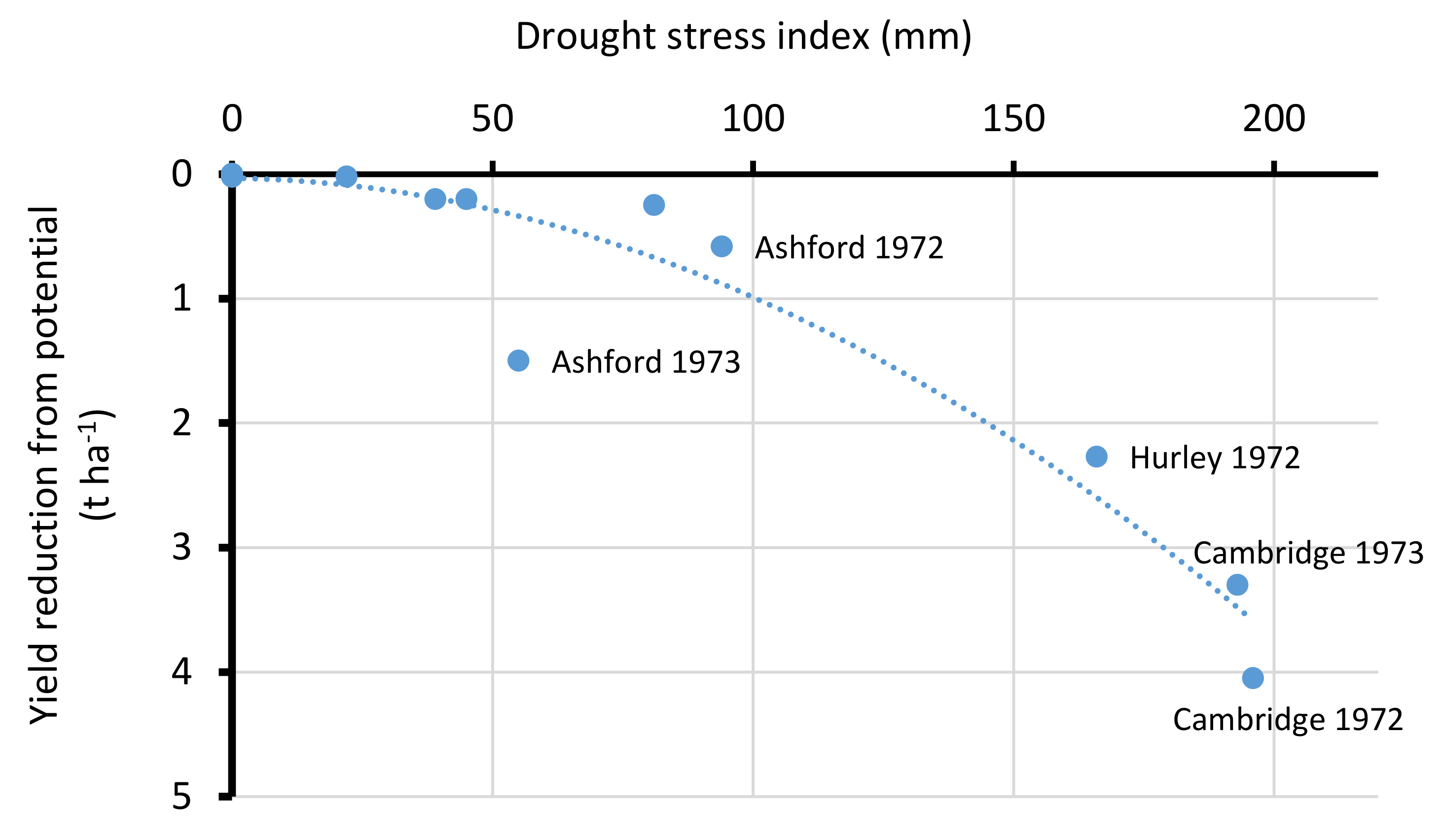
| Site | Year | DM Yield Decrease | |
|---|---|---|---|
| Cambridge | 1972 | 4.05 | a |
| Cambridge | 1973 | 3.30 | ab |
| Hurley | 1972 | 2.27 | bc |
| Ashford | 1973 | 1.50 | cd |
| Ashford | 1972 | 0.58 | de |
| Hurley | 1973 | 0.25 | de |
| Oxford | 1972 | 0.20 | de |
| H.Mowthorpe | 1972 | 0.20 | de |
| Oxford | 1973 | 0.02 | de |
| Winchester | 1973 | 0.02 | de |
| Stratford | 1972 | 0.02 | de |
| Stratford | 1973 | 0.02 | de |
| Morpeth | 1973 | 0.02 | de |
| H.Mowthorpe | 1973 | 0.00 | de |
| Leeds | 1972 | 0.00 | de |
| Leeds | 1973 | 0.00 | de |
| Morpeth | 1972 | 0.00 | de |
| Newton Abbot | 1972 | 0.00 | de |
| Winchester | 1972 | 0.00 | de |
| Aberystwyth | 1973 | 0.00 | e |
| Newton Abbot | 1973 | 0.00 | e |
References
- Havlík, P.; Valin, H.; Herrero, M.; Obersteiner, M.; Schmid, E.; Rufino, M.C.; Mosnier, A.; Thornton, P.K.; Böttcher, H.; Conant, R.T.; et al. Climate change mitigation through livestock system transitions. Proc. Natl. Acad. Sci. USA 2014, 111, 3709–3714. [Google Scholar] [CrossRef] [Green Version]
- Lugato, E.; Panagos, P.; Bampa, F.; Jones, A.; Montanarella, L. A new baseline of organic carbon stock in European agricultural soils using a modelling approach. Glob. Chang. Biol. 2013, 20, 313–326. [Google Scholar] [CrossRef] [PubMed]
- Huyghe, C.; De Vliegher, A.; van Gils, B.; Peeters, A. Grasslands and Herbivore Production in Europe and Effects of Common Policies; Editions Quae: Versailles, France, 2014. [Google Scholar]
- Soussana, J.; Tallec, T.; Blanfort, V. Mitigating the greenhouse gas balance of ruminant production systems through carbon sequestration in grasslands. Animal 2010, 4, 334–350. [Google Scholar] [CrossRef] [PubMed] [Green Version]
- Scollan, N.D.; Greenwood, P.L.; Newbold, C.J.; Ruiz, D.R.Y.; Shingfield, K.J.; Wallace, R.J.; Hocquette, J.-F. Future research priorities for animal production in a changing world. Anim. Prod. Sci. 2011, 51, 1–5. [Google Scholar] [CrossRef]
- Smith, P. Do grasslands act as a perpetual sink for carbon? Glob. Chang. Biol. 2014, 20, 2708–2711. [Google Scholar] [CrossRef] [PubMed]
- Lüscher, A.; Fuhrer, J.; Newton, P.C.D. Global atmospheric change and its effect on managed grassland systems. In Grassland—A Global Resource; McGilloway, D.A., Ed.; Academic Publishers: Wageningen, The Netherlands, 2005; pp. 251–264. [Google Scholar]
- Buttler, A.; Mariotte, P.; Meisser, M.; Guillaume, T.; Signarbieux, C.; Vitra, A.; Preux, S.; Mercier, G.; Quezada, J.; Bragazza, L.; et al. Drought-induced decline of productivity in the dominant grassland species Lolium perenne L. depends on soil type and prevailing climatic conditions. Soil Biol. Biochem. 2019, 132, 47–57. [Google Scholar] [CrossRef]
- Perera, R.S.; Cullen, B.R.; Eckard, R.J. Using Leaf Temperature to Improve Simulation of Heat and Drought Stresses in a Biophysical Model. Plants 2019, 9, 8. [Google Scholar] [CrossRef] [Green Version]
- Rounsevell, M.; Brignall, A.; Siddons, P. Potential climate change effects on the distribution of agricultural grassland in England and Wales. Soil Use Manag. 1996, 12, 44–51. [Google Scholar] [CrossRef]
- Riedo, M.; Gyalistras, D.; Fischlin, A.; Fuhrer, J. Using an ecosystem model linked to GCM-derived local weather scenarios to analyse effects of climate change and elevated CO2 on dry matter production and partitioning, and water use in temperate managed grasslands. Glob. Chang. Biol. 1999, 5, 213–223. [Google Scholar] [CrossRef] [Green Version]
- Morales, P.; Hickler, T.; Rowell, D.P.; Smith, B.; Sykes, M.T. Changes in European ecosystem productivity and carbon balance driven by regional climate model output. Glob. Chang. Biol. 2006, 13, 108–122. [Google Scholar] [CrossRef]
- Geris, J.; Tetzlaff, D.; McDonnell, J.; Soulsby, C. The relative role of soil type and tree cover on water storage and transmission in northern headwater catchments. Hydrol. Process. 2014, 29, 1844–1860. [Google Scholar] [CrossRef] [Green Version]
- Garwood, E.A.; Williams, T.E. Soil water use and growth of a grass sward. J. Agric. Sci. 1967, 68, 281–292. [Google Scholar] [CrossRef]
- Lin, H. Earth’s Critical Zone and hydropedology: Concepts, characteristics, and advances. Hydrol. Earth Syst. Sci. 2010, 14, 25–45. [Google Scholar] [CrossRef] [Green Version]
- Binnie, R.C.; Harrington, F.J. The effect of cutting height and cutting frequency on the productivity of an Italian ryegrass sward. Grass Forage Sci. 1972, 27, 177–182. [Google Scholar] [CrossRef]
- Wilman, D.; Droushiotis, D.; Koocheki, A.; Lwoga, A.B.; Shim, J.S. The effect of interval between harvests and nitrogen application on the digestibility and digestible yield and nitrogen content and yield of four ryegrass varieties in the first harvest year. J. Agric. Sci. 1976, 86, 393–399. [Google Scholar] [CrossRef]
- Herrmann, A.; Kelm, M.; Kornher, A.; Taube, F. Performance of grassland under different cutting regimes as affected by sward composition, nitrogen input, soil conditions and weather—A simulation study. Eur. J. Agron. 2005, 22, 141–158. [Google Scholar] [CrossRef]
- Crider, F.J. Root-Growth Stoppage Resulting from Defoliation of Grass; USDA Technical Bulletin No. 1102; USDA: Washington, WA, USA, 1955.
- Davidson, J.L.; Milthorpe, F.L. Carbohydrate reserves in the regrowth of cocksfoot (Dactylis glomerate L.). J. Br. Orassld Soc. 1965, 20, 15–18. [Google Scholar] [CrossRef]
- Wilman, D.; Mohamed, A.A. Response to nitrogen application and interval between harvests in five grasses? Leaf development. Nutr. Cycl. Agroecosyst. 1981, 2, 3–20. [Google Scholar] [CrossRef]
- Lamsal, A.; Welch, S.; Jones, J.; Boote, K.; Asebedo, A.; Crain, J.; Wang, X.; Boyer, W.; Giri, A.; Frink, E.; et al. Efficient crop model parameter estimation and site characterization using large breeding trial data sets. Agric. Syst. 2017, 157, 170–184. [Google Scholar] [CrossRef]
- Jones, J.W.; Antle, J.M.; Basso, B.; Boote, K.J.; Conant, R.T.; Foster, I.; Godfray, H.C.J.; Herrero, M.; Howitt, R.E.; Janssen, S.; et al. Toward a new generation of agricultural system data, models, and knowledge products: State of agricultural systems science. Agric. Syst. 2017, 155, 269–288. [Google Scholar] [CrossRef]
- Qi, A.; Murray, P.J.; Richter, G.M. Modelling productivity and resource use efficiency for grassland ecosystems in the UK. Eur. J. Agron. 2017, 89, 148–158. [Google Scholar] [CrossRef]
- Basso, B.; Dumont, B.; Maestrini, B.; Shcherbak, I.; Robertson, G.P.; Porter, J.R.; Smith, P.; Paustian, K.; Grace, P.R.; Asseng, S.; et al. Soil Organic Carbon and Nitrogen Feedbacks on Crop Yields under Climate Change. Agric. Environ. Lett. 2018, 3, 180026. [Google Scholar] [CrossRef] [Green Version]
- Schapendonk, A.; Stol, W.; Van Kraalingen, D.; Bouman, B. LINGRA, a sink/source model to simulate grassland productivity in Europe. Eur. J. Agron. 1998, 9, 87–100. [Google Scholar] [CrossRef]
- Rodriguez, D.; Van Oijen, M.; Schapendonk, A.H.M.C. LINGRA-CC: A sink-source model to simulate the impact of climate change and management on grassland productivity. New Phytol. 1999, 144, 359–368. [Google Scholar] [CrossRef]
- Wolf, J. Users Guide for LINGRA-N: Simple Generic Model for Simulation of Crop Growth under Potential, Water Limited and Nitrogen Limited Conditions. 2012. Available online: https://models.pps.wur.nl/lingra-n-grassland-model-potential-water-limited-and-n-limited-conditions-fortran (accessed on 15 January 2019).
- Burgess, P.J.; Giannitsopoulos, M.L.; Richter, G.M.; Topp, C.F.E.; Bell, M.; Takahashi, T.; Ingram, J. Modelling Grass Growth with LINGRA-N-Plus: Teaching Guide; Cranfield University: Oxfordshire, UK, 2020; 23p, Available online: https://cord.cranfield.ac.uk/articles/software/Data_underpinning_NERC_Research_Translation_Grassland_Management_project/11359613?file=24173714 (accessed on 14 September 2020).
- Kersebaum, K. Application of a simple management model to simulate water and nitrogen dynamics. Ecol. Model. 1995, 81, 145–156. [Google Scholar] [CrossRef]
- Addiscott, T.M.; Whitmore, A.P. Computer simulation of changes in soil mineral nitrogen and crop nitrogen during autumn, winter and spring. J. Agric. Sci. 1987, 109, 141–157. [Google Scholar] [CrossRef]
- Stanford, G.; Smith, S.J. Nitrogen mineralization potentials of soils. Soil Sci. Am. J. Proc. 1972, 36, 465–472. [Google Scholar] [CrossRef]
- Abdelmagid, H.M. Factors Affecting Nitrogen Mineralization and Nitrate Reduction in Soils. Master’s Thesis, Iowa State University, Ames, IA, USA, 1980. Retrospective Theses and Dissertations. Available online: https://lib.dr.iastate.edu/rtd/6820 (accessed on 23 November 2020).
- Morrison, J.; Jackson, M.V.; Sparrow, P.E. The Response of Perennial Ryegrass to Fertilizer Nitrogen in Relation to Climate and Soil. Report of the joint ADAS/GRI Grassland Manuring Trial–GM 20; Technical Report No 27; February 1980; Grassland Research Institute, ADAS and Rothamsted Experimental Station: Harpenden, UK, 1980; Available online: https://www.worldcat.org/title/response-of-perennial-ryegrass-to-fertilizer-nitrogen-in-relation-to-climate-and-soil-report-of-the-joint-adasgri-grassland-manuring-trial-gm-20/oclc/838477580 (accessed on 20 March 2019).
- Nüske, A.; Richter, J. N-mineralization in Löss-Parabrownearthes: Incubation experiments. Plant Soil 1981, 59, 237–247. [Google Scholar] [CrossRef]
- Richter, G.; Hoffmann, A.; Nieder, R.; Richter, J. Nitrogen mineralization in loamy arable soils after increasing the ploughing depth and ploughing grasslands. Soil Use Manag. 1989, 5, 169–173. [Google Scholar] [CrossRef]
- Gustavsson, A. A developmental scale for perennial forage grasses based on the decimal code framework. Grass Forage Sci. 2011, 66, 93–108. [Google Scholar] [CrossRef]
- Brown, I.; Poggio, L.; Gimona, A.; Castellazzi, M. Climate change, drought risk and land capability for agriculture: Implications for land use in Scotland. Reg. Environ. Chang. 2011, 11, 503–518. [Google Scholar] [CrossRef]
- Perryman, S.A.M.; Castells-Brooke, N.I.D.; Glendining, M.J.; Goulding, K.W.T.; Hawkesford, M.J.; Macdonald, A.J.; Ostler, R.J.; Poulton, P.R.; Rawlings, C.J.; Scott, T.; et al. The electronic Rothamsted Archive (e-RA), an online resource for data from the Rothamsted long-term experiments. Sci. Data 2018, 5, 180072. [Google Scholar] [CrossRef] [Green Version]
- Harrison, A.F.; Howard, D.M.; Lawson, G.J. UK Soils: Their Phosphorus Sorption Capacity and Potential for P Removal from Sewage Effluents in Emergent Hydrophyte Treatment Systems; NERC/Institute of Terrestrial Ecology: London, UK, 1988; 179p, Available online: http://nora.nerc.ac.uk/id/eprint/6204/1/HarrisonT01014a5N006204CR.pdf (accessed on 16 March 2020).
- Cranfield University. The Soils Guide; Cranfield University: Cranfield, UK, 2020; Available online: www.landis.org.uk (accessed on 8 November 2020).
- R Core Team. R: A Language and Environment for Statistical Computing; R Foundation for Statistical Computing: Vienna, Austria, 2018; Available online: https://www.R-project.org (accessed on 14 January 2019).
- Smith, P.; Smith, J.; Powlson, D.; McGill, W.; Arah, J.; Chertov, O.; Coleman, K.; Franko, U.; Frolking, S.; Jenkinson, D.; et al. A comparison of the performance of nine soil organic matter models using datasets from seven long-term experiments. Geoderma 1997, 81, 153–225. [Google Scholar] [CrossRef]
- Johannes, A.; Matter, A.; Schulin, R.; Weisskopf, P.; Baveye, P.C.; Boivin, P. Optimal organic carbon values for soil structure quality of arable soils. Does clay content matter? Geoderma 2017, 302, 14–21. [Google Scholar] [CrossRef]
- Prout, J.M.; Shepherd, K.D.; McGrath, S.P.; Kirk, G.J.D.; Haefele, S.M. What is a good level of soil organic matter? An index based on organic carbon to clay ratio. Eur. J. Soil Sci. 2020, 1–11. [Google Scholar] [CrossRef]
- Topp, C.F.E.; Doyle, C.J. Modelling the comparative productivity and profitability of grass and legume systems of silage production in northern Europe. Grass Forage Sci. 2004, 59, 274–292. [Google Scholar] [CrossRef]
- National Soil Resources Institute. Impacts of Climate Change on Soil Functions (Project code SP0538); Report for DEFRA; Department for Environment, Food and Rural Affairs: London, UK, 2005.
- Abassi, M.K.; Kazmi, M.; Hussan, F.U. Nitrogen Use Efficiency and Herbage Production of an Established Grass Sward in Relation to Moisture and Nitrogen Fertilization. J. Plant Nutr. 2005, 28, 1693–1708. [Google Scholar] [CrossRef]
- Waraich, E.A.; Ahmad, R.; Ashraf, M.Y. Role of mineral nutrition in alleviation of drought stress in plants. Aust. J. Crop Sci. 2011, 5, 764–777. [Google Scholar]
- Lowe, J.; Bernie, D.; Bett, P.; Bricheno, L.; Brown, S.; Calvert, D.; Clark, R.; Eagle, K.; Edwards, T.; Fosser, G.; et al. UKCP18 Science Overview Report, November 2018 (Updated March 2019). Available online: https://www.metoffice.gov.uk/pub/data/weather/uk/ukcp18/science-reports/UKCP18-Land-report.pdf (accessed on 14 November 2020).
- Armstrong, A.; Castle, D. Potential impacts of climate change on patterns of production and the role of drainage in grassland. Grass Forage Sci. 1992, 47, 50–61. [Google Scholar] [CrossRef]
- Gregory, A.S.; Webster, C.P.; Watts, C.W.; Whalley, W.R.; MacLeod, C.J.A.; Joynes, A.; Papadopoulos, A.; Haygarth, P.M.; Binley, A.; Humphreys, M.W.; et al. Soil Management and Grass Species Effects on the Hydraulic Properties of Shrinking Soils. Soil Sci. Soc. Am. J. 2010, 74, 753–761. [Google Scholar] [CrossRef] [Green Version]
- Kodešová, R.; Jirků, V.; Kodeš, V.; Mühlhanselová, M.; Nikodem, A.; Žigová, A. Soil structure and soil hydraulic properties of Haplic Luvisol used as arable land and grassland. Soil Tillage Res. 2011, 111, 154–161. [Google Scholar] [CrossRef]
- Lassaletta, L.; Billen, G.; Grizzetti, B.; Anglade, J.; Garnier, J. 50 Year trends in nitrogen use efficiency of world cropping systems: The relationship between yield and nitrogen input to cropland. Environ. Res. Lett. 2014, 9, 105011. [Google Scholar] [CrossRef]
- Swaney, D.P.; Howarth, R.W.; Hong, B. Nitrogen use efficiency and crop production: Patterns of regional variation in the United States, 1987–2012. Sci. Total Environ. 2018, 635, 498–511. [Google Scholar] [CrossRef] [PubMed]
- Ashman, M.R.; Geeta, P. Essential Soil Science. A Clear and Concise Introduction to Soil Science; Blackwell Science: Oxford, UK, 2002. [Google Scholar]
- Tremblay, N.; Bouroubi, Y.M.; Bélec, C.; Mullen, R.W.; Kitchen, N.R.; Thomason, W.E.; Ebelhar, S.; Mengel, D.B.; Raun, W.R.; Francis, D.D.; et al. Corn Response to Nitrogen is Influenced by Soil Texture and Weather. Agron. J. 2012, 104, 1658–1671. [Google Scholar] [CrossRef] [Green Version]
- Hassink, J. Effects of soil texture and grassland management on soil organic C and N and rates of C and N mineralization. Soil Biol. Biochem. 1994, 26, 1221–1231. [Google Scholar] [CrossRef]
- Withers, P.; Sylvester-Bradley, R. Nitrogen fertilizer requirements of cereals following grass. Soil Use Manag. 2006, 15, 221–229. [Google Scholar] [CrossRef]

| Site | Total Rainfall (mm) | Mean Temperature (°C) | Total Radiation (GJ m−2) | Rooting Depth (cm) | AWC (mm) | Max PSMD (mm) | DSI (mm) | |||||
|---|---|---|---|---|---|---|---|---|---|---|---|---|
| 1972 | 1973 | 1972 | 1973 | 1972 | 1973 | 1972 | 1973 | 1972 | 1973 | |||
| Aberystwyth | - | 1055 | - | 9.8 | - | 3.16 | 125 | 160 | - | 74 | - | 0 |
| Morpeth | 577 | 522 | 8.0 | 8.4 | 2.78 | 2.87 | 100 | 140 | 125 | 87 | 0 | 0 |
| High Mowthorpe | 633 | 613 | 7.8 | 8.2 | 2.87 | 2.93 | 45 | 81 | 120 | 75 | 39 | 0 |
| Leeds | 544 | 505 | 8.8 | 9.2 | 2.81 | 3.26 | 100 | 188 | 107 | 116 | 0 | 0 |
| Cambridge | 419 | 408 | 9.6 | 9.9 | 3.24 | 3.51 | 60 | 24 | 220 | 217 | 196 | 193 |
| Newton Abbot | 1341 | 869 | 9.9 | 10.4 | 3.42 | 3.42 | 100 | 128 | 91 | 73 | 0 | 0 |
| Oxford | 576 | 495 | 9.9 | 10.2 | 3.01 | 3.42 | 100 | 180 | 225 | 202 | 45 | 22 |
| Hurley | 596 | 548 | 9.5 | 9.7 | 3.33 | 3.28 | 60 | 60 | 226 | 141 | 166 | 81 |
| Ashford | 717 | 583 | 9.1 | 9.6 | 3.29 | 3.54 | 90 | 115 | 170 | 209 | 55 | 94 |
| Stratford | 593 | 482 | 9.1 | 9.5 | 3.47 | 3.54 | 100 | 160 | 75 | 54 | 0 | 0 |
| Winchester | 813 | 546 | 9.4 | 10.3 | 3.22 | 3.54 | 100 | 160 | 150 | 52 | 0 | 0 |
| Site | Series | Soil Texture | Previous Crop * | Total Soil N | Nrpm |
|---|---|---|---|---|---|
| (kg ha−1) | (kg ha−1) | ||||
| Aberystwyth | Conway # | Silt | PG | 8160 | 163 |
| Morpeth | Dunkeswick | Sandy loam over silt loam | PG | 7920 | 163 |
| H. Mowthorpe | Andover | Silt to silty clay | AR, PR | 8400 | 158 |
| Leeds | Aberford | Clay loam over clay | AR | 4800 | 96 |
| Cambridge | Landbeach | Sandy loam over sandy clay loam | AR | 6960 | 139 |
| N. Abbot | HighWeek | Silt | Ley, AR | 8160 | 163 |
| Oxford | Thames | Loam | AR | 6960 | 139 |
| Hurley | Frilsham | Sandy loam | AR | 4320 | 86 |
| Ashford | Thorne | Silt loam | AR | 5520 | 110 |
| Stratford | Evesham | Clay loam | Ley, AR | 8160 | 163 |
| Winchester | Winchester | Clay loam | AR | 6240 | 125 |
| Site | SOM | Total N | C:N * | Clay + | SOC/Clay * | SOC/Clay Designation |
|---|---|---|---|---|---|---|
| (%) | (%) | (%) | ||||
| Aberystwyth | 10.5 | 0.34 | 18.0 | 31 | 0.20 | Very good |
| Morpeth | 10.5 | 0.33 | 18.5 | 24 | 0.25 | Very good |
| H. Mowthorpe | 6.2 | 0.35 | 10.3 | 41 | 0.09 | Moderate |
| Leeds | 3.2 | 0.20 | 9.3 | 25 | 0.07 | Moderate |
| Cambridge | 4.5 | 0.29 | 9.0 | 12 | 0.22 | Very good |
| N. Abbot | 5.6 | 0.34 | 9.6 | 10 | 0.33 | Very good |
| Oxford | 4.8 | 0.29 | 9.6 | 52 | 0.05 | Degraded |
| Hurley | 2.6 | 0.18 | 8.4 | 26 | 0.06 | Degraded |
| Ashford | 3.7 | 0.24 | 9.0 | 14 | 0.15 | Very good |
| Stratford | 5.9 | 0.34 | 10.1 | 52 | 0.06 | Degraded |
| Winchester | 3.9 | 0.26 | 8.7 | 53 | 0.04 | Degraded |
| Descriptive Statistics | 1973 | 1972 | ||||
|---|---|---|---|---|---|---|
| Wilman et al. | Morrison et al. | Morrison et al. | ||||
| LINGRA-N-Plus | LINGRA-N | LINGRA-N-Plus | LINGRA-N | LINGRA-N-Plus | LINGRA-N | |
| Constant | −0.03 | 0.74 | 0.25 | −0.65 | 1.66 | 1.32 |
| Slope | 0.93 *** | 0.79 *** | 1.12 *** | 1.38 *** | 0.96 *** | 1.21 *** |
| R2 | 0.946 | 0.748 | 0.844 | 0.821 | 0.775 | 0.743 |
| RMSE | 1.08 | 2.22 | 1.98 | 3.21 | 2.45 | 3.91 |
| EF | 0.92 | 0.67 | 0.65 | −0.06 | 0.58 | −0.06 |
| N Applied (kg N ha−1) | Total Harvested Yield (t ha−1) | |||
|---|---|---|---|---|
| 1972 | 1973 | |||
| “Non-Droughty” Sites | “Droughty” Sites | “Non-droughty” Sites | “Droughty” Sites | |
| 0 | 2.96 de | 1.52 e | 3.10 e | 1.92 e |
| 150 | 6.14 c | 4.08 d | 6.50 cd | 5.30 d |
| 300 | 9.74 ab | 6.90 c | 10.05 a | 7.80 bc |
| 450 | 11.14 a | 8.92 b | 10.55 a | 9.25 ab |
| N Application (kg N ha−1) | Morpeth * | High Mowthorpe | Cambridge | Oxford | Hurley | |
|---|---|---|---|---|---|---|
| N uptake | 0 | 39 | 24 | 13 | 32 | 21 |
| (kg N ha−1) | 150 | 215 | 128 | 115 | 135 | 124 |
| 300 | 296 | 233 | 196 | 239 | 228 | |
| 450 | 296 | 266 | 225 | 343 | 333 | |
| Incremental N | 0 to 150 | 0.48 | 0.81 | 0.89 | 0.76 | 0.83 |
| uptake efficiency | 150 to 300 | 0.27 | 0.45 | 0.41 | 0.44 | 0.46 |
| (kg N (kg N)−1) | 300 to 450 | 0.00 | 0.12 | 0.13 | 0.30 | 0.32 |
| Nitrogen Application (kg N ha−1) | Observed Yield (t ha−1) | Predicted Yield (t ha−1) | |||
|---|---|---|---|---|---|
| HI = 28 d; RD = 60 cm | HI = 28 d; RD = 60 cm | HI = 28 d; RD = 90 cm | HI = 35 d; RD = 60 cm | HI = 35; RD = 90 cm | |
| 0 | 2.7 | 1.0 | 1.0 | 0.9 | 0.9 |
| 150 | 4.1 | 5.8 | 6.2 | 5.7 | 6.3 |
| 300 | 7.2 | 7.3 | 8.4 | 7.6 | 8.4 |
| 450 | 7.6 | 7.6 | 8.9 | 8.0 | 9.2 |
Publisher’s Note: MDPI stays neutral with regard to jurisdictional claims in published maps and institutional affiliations. |
© 2021 by the authors. Licensee MDPI, Basel, Switzerland. This article is an open access article distributed under the terms and conditions of the Creative Commons Attribution (CC BY) license (https://creativecommons.org/licenses/by/4.0/).
Share and Cite
Giannitsopoulos, M.L.; Burgess, P.J.; Richter, G.M.; Bell, M.J.; Topp, C.F.E.; Ingram, J.; Takahashi, T. Modelling the Interactions of Soils, Climate, and Management for Grass Production in England and Wales. Agronomy 2021, 11, 677. https://doi.org/10.3390/agronomy11040677
Giannitsopoulos ML, Burgess PJ, Richter GM, Bell MJ, Topp CFE, Ingram J, Takahashi T. Modelling the Interactions of Soils, Climate, and Management for Grass Production in England and Wales. Agronomy. 2021; 11(4):677. https://doi.org/10.3390/agronomy11040677
Chicago/Turabian StyleGiannitsopoulos, Michail L., Paul J. Burgess, Goetz M. Richter, Matt J. Bell, Cairistiona F. E. Topp, Julie Ingram, and Taro Takahashi. 2021. "Modelling the Interactions of Soils, Climate, and Management for Grass Production in England and Wales" Agronomy 11, no. 4: 677. https://doi.org/10.3390/agronomy11040677