Abstract
Cut flower production in the Bogotá savanna is one of Colombia’s main export products. Flower production is mainly carried out in greenhouses, as this type of production system has substantial advantages over crops grown in open fields. Protected agriculture provides timely climate management that improves crop yields. The objective of this work was to build and validate a 3D CFD numerical model to understand the spatial distribution of temperatures because of the air flow dynamics inside a typical greenhouse in the Bogotá savanna. Root mean square error (RMSE) and mean absolute percentage error (MAPE) were the statistical indicators used between experimental and simulated wind speed and temperature data. The simulations considered twelve evaluation scenarios that were established based on the climatic conditions characteristic of the study region. The results indicate that under regional conditions of temperature and wind for this type of passive greenhouse, there is a deficient ventilation rate. This rate does not exceed 35 exchanges h−1 compared to the recommended rates for crops, which is between 45 and 60 air exchanges h−1. This renewal rate contributes to the heterogeneity of the microclimatic dynamics of the greenhouse, presenting hot spots with temperature values above 32 °C in all examined scenarios. For the lower air speed scenarios (<1 ms−1), these areas of high temperature can reach up to 50% of the cultivated area. Therefore, it is suggested that future studies should seek technical solutions to optimize the microclimatic conditions of the greenhouse design used in the Colombian floriculture sector.
1. Introduction
One of the most relevant characteristics that influence the performance of crops grown in covered agricultural production systems is the generated microclimate inside the different kinds of greenhouse designs used around the world [1,2]. Microclimate conditions generated inside the structure will be dependent on the air flow patterns, the climatic conditions of the external environment, and the heat and mass exchanges between the plants and the soil and also between the plants and the air [3].
Therefore, these microclimate conditions will positively or negatively affect physiological processes, such as photosynthesis and evapotranspiration, that directly influence the growth and development of the crop [4,5]. In Colombia, covered agriculture in the ornamental and cut flower sector is mainly performed in passive greenhouses [6]. Within this typology of greenhouses, the most used type of structure is the traditional Colombian structure, which was developed in the beginning of the ornamental sector in the 60s and is built with a pitched roof and structural materials such as wood [7].
The main disadvantage of this greenhouse is its low capacity for microclimate management and its highly heterogeneous microclimate behavior [8]. In the traditional Colombian greenhouse, microclimatic management is carried out through the opening and closing of ventilation areas located on the four sides of the greenhouse, trying to take advantage of the air flows generated by wind or thermal buoyancy that are part the phenomenon of natural ventilation [8,9].
One of the most important variables to be analyzed inside greenhouses is temperature, which directly influences the growth and development of plants and, at the same time, influences the post-harvest quality of harvested products [10,11,12]. Therefore, it is necessary for researchers and producers in the area of protected agriculture to know the magnitude of the temperature values generated and the spatial distribution of the temperature inside the greenhouse [6,10]. For the traditional Colombian greenhouse, it is known through experimental studies that there are deficiencies and thermal heterogeneity in this type of structure, although it should be noted that the study of flow patterns and the quantification of the airflow rates of this type of greenhouse is limited.
Natural ventilation is a microclimate management method widely used globally, mainly because it is a low-cost and low-environmental-impact method [13]. The study and quantification of ventilation in greenhouses has been carried out from various researchers and include in situ experimentation and laboratory experimentation and, from the use of different modeling and simulation techniques, as can be reviewed in the work developed by Akrami et al. [14].
Among the modeling and simulation methodologies, one of the most widely implemented due to its maturity and robustness is computational fluid dynamics (CFD). This simulation technique, once validated, visualizes the behavior of air flow patterns, quantifies ventilation rates, and the spatial distribution of the air temperature throughout the interior volume of the greenhouse. In addition, it also allows evaluating unconstructed scenarios, which makes it a very interesting tool for the design or optimization of ventilation systems [3,7].
Therefore, the objective of this research was focused on implementing and validating a 3D CFD model to evaluate the behavior of air flow and the spatial distribution of temperature inside a traditional Colombian greenhouse used for the production of cut flowers in the Colombian savannah of Bógota.
2. Materials and Methods
2.1. Description of the Experimental Greenhouse
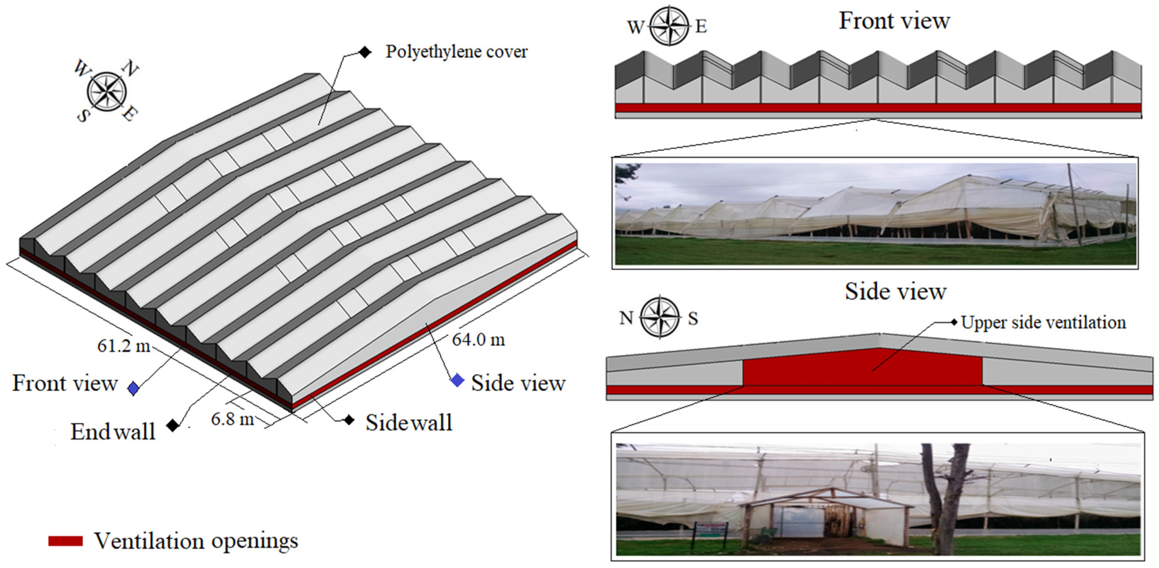
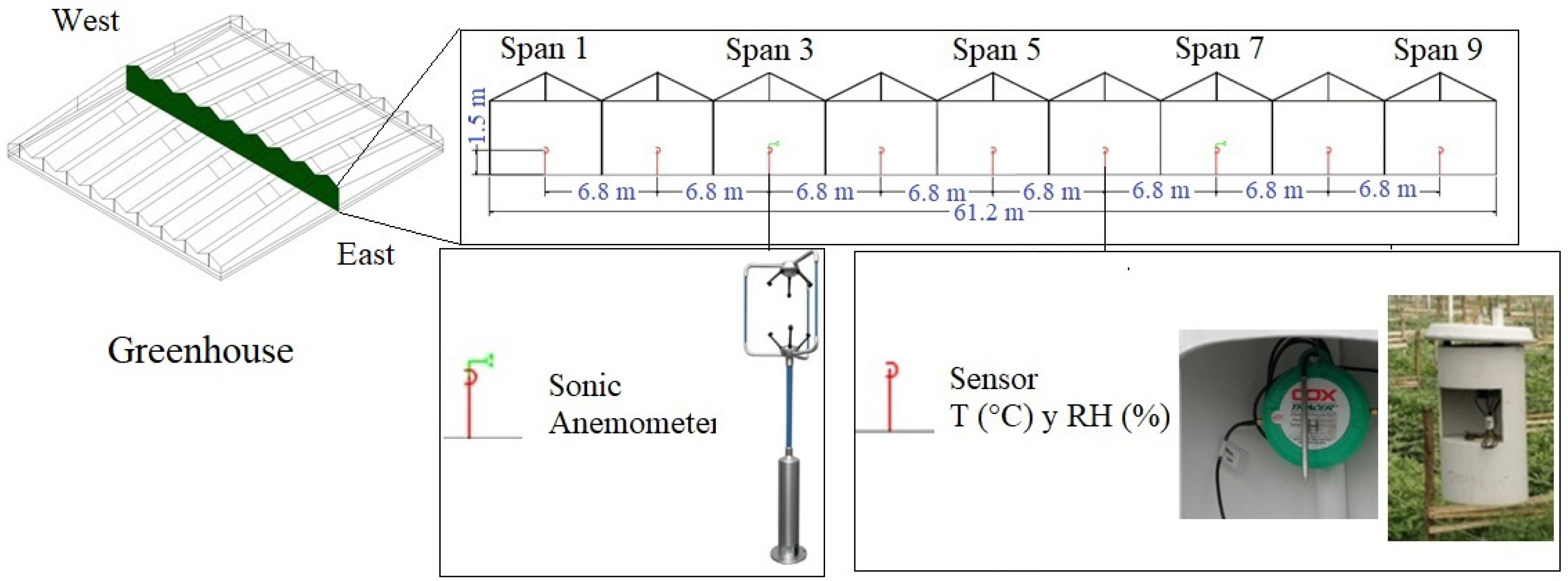
The research was carried out in a traditional Colombian greenhouse with a 200 µm thick clear polyethylene cover and a covering with an area of 3916.8 m2 of covered soil. This greenhouse prototype belonged to a commercial farm producing cut flowers located in the municipality of Guasca, department of Cundinamarca, in the Andean region of Colombia. The greenhouse consisted of 9 spans of 6.80 m wide attached in the transverse direction (W-E) for a width of 61.2 m, while the longitudinal dimension was 64.0 m and was in the N-S direction (Figure 1).

Figure 1.
Overall dimensions of the greenhouse evaluated.
The greenhouse had ventilation openings on the sidewalls and endwalls with an effective vertical opening of 1.1 m, resulting in a ventilation surface area of 275.4 m2. This ventilation area was complemented by an upper ventilation area located on the west side of the greenhouse of 51.5 m2, which brought the total ventilation area to 8.34% of the covered floor area. These ventilation areas are managed based the producers’ own criteria. In general, these ventilation areas are opened manually in the early morning hours (6:00 or 7:00 h), and they are also closed manually in the afternoon hours (15:00 or 16:00 h) or at the time of rainfall. The minimum and maximum heights above the gutter were 3.0 m and 4.5 m and above the ridge roof 4.7 m and 6.2 m, respectively.
2.2. Climatic Characteristics of the Study Region
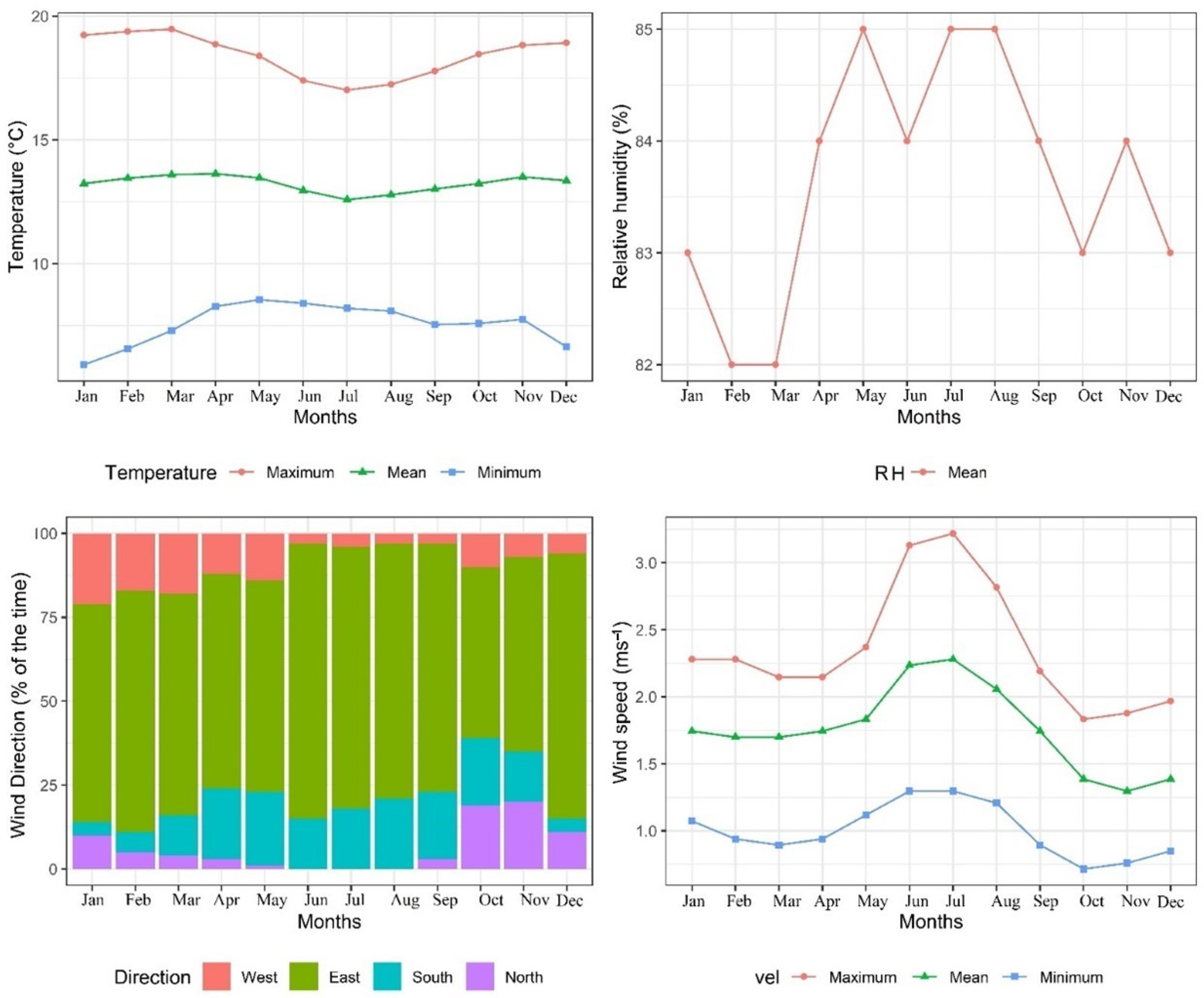
Figure 2 shows the annual variation of the several climatic variables calculated from 30 years of historical data. The average temperature presents a value of 13.23 °C with mean maximum and minimum values of 18.45 °C and 7.53 °C. The average relative humidity value is 83.6%. These values coincide with those reported by Cortés-Rojas et al. [15].
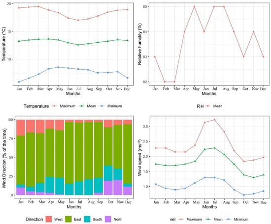
Figure 2.
Annual variation of the main meteorological variables in the study region.
For the wind speed, the mean value was 0.99 ms−1, and the average maximum and minimum values were 2.35 ms−1 and 1.75 ms−1, respectively. The dominant wind direction is from the east (E), accounting for more than 50% of the accounting measurements in each of the months. For the remaining directions, the percentage of events for each of them is less than 25% (Figure 2). Finally, solar radiation has an annual average value of 187 Wm−2, with maximum values reaching 650 Wm−2 between 11:00 and 14:00, h as reported by Medina Campos et al. [16].
2.3. CFD Modeling
Construction and Discretization of the Computational Domain
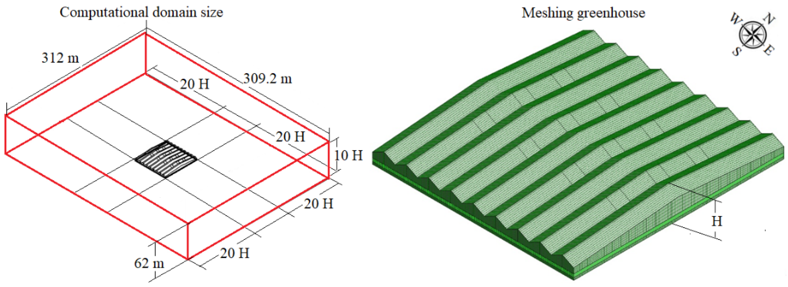
This stage started with the geometrical construction of the evaluated greenhouse and a large computational domain around each of the walls and the roof of the structure. The criterion used for the construction of the computational domain was the maximum height (H = 6.2 m) of the greenhouse (Figure 3), for which it was defined that, according to the objective of this research work, each of the edges of the greenhouse should be separated at a distance of 20 H, a value that is higher than the minimum of 15 H recommended for the leeward side of the computational domain [17].

Figure 3.
Computational domain dimensions and greenhouse meshing.
For the length of the height, the recommendation used in several works on natural ventilation was followed. It was defined that the top of the computational domain should be at a minimum distance of 10 H with respect to the boundary considered as the greenhouse floor [18]. These dimensions guarantee adequate solutions of the air flow patterns based on the outdoor environment and their interaction with the ventilation openings greenhouse. This approach also allows modeling in a coupled way the effects on the air flow patterns caused by the wind effect of the natural ventilation in the outdoor environment and those of the thermal effects generated inside the greenhouse [19].
In a subsequent step, the process of meshing computational domain and the greenhouse was carried out, for which an unstructured numerical grid of rectangular elements was used. Separate zones with refined sizes near the floor, the roof, and the ventilation areas of the greenhouse, where the most important thermal gradients are present in each simulated scenario, were established. The total number of elements of the numerical grid was 6,195,432. This size was determined once a test of independence of the solution to the total size of the numerical grid was performed.
This procedure was carried out in accordance with the natural ventilation study developed by Villagrán et al. [4]. For our research, a total of 10 numerical grids were evaluated, ranging in size from 1,050,381 to 14,603,942 elements. Therefore, the numerical grid-size independence test allowed us to establish the size that generated the lowest computational cost for a solution with acceptable accuracy and without convergence problems [20,21]. It should be noted that, in order to perform this independence test, it is very valuable to collect the experimental data inside the evaluated greenhouse. This is mainly due to the fact that a better selection of the size of the numerical grid can be made, and simultaneously, the first analysis of the predictive capacity of the generated CFD model can be performed.
In addition, another factor that has a high impact on the accuracy of the results is the quality of the elements of the numerical grid [22,23]. In this case, as an evaluation criterion, the orthogonality of the cells was rated, finding that 93.2% of the elements had a value higher than 0.91 and an average asymmetry of 0.11. These values establish that the numerical grid is composed of high quality elements [24,25]. It should be noted that to achieve these values, it is necessary to check the numerical grid and redesign some cells mainly near the roof region where, due to the shape of the greenhouse, the cells tend to lose their aspect ratio.
The boundary conditions established were symmetry boundary for the edges of the computational domain that are parallel to the air flow and enhanced wall boundary for the floor, roof, and wall areas in the greenhouse as well as for the floor of the computational domain around the greenhouse. For the ventilation areas arranged in the structure, an interior-type boundary condition was established, while in the case of the computational domain roof region, a wall boundary condition with a solar radiation flux was established.
At the windward boundary, an air inlet velocity condition was established by setting a logarithmic wind profile using a user-defined function (UDF), as successfully implemented in the work developed by Villagrán and Bojacá. [26]. Finally, at the leeward boundary, a pressure and airflow outflow condition was also established. For the materials included in the computational domain, such as air, soil, and polyethylene film, the physical, thermal, and optical properties summarized in Table 1 were imposed.

Table 1.
Properties of computational domain materials.
2.4. Physical Models and Governing Equations
The development of the three-dimensional numerical solution for the behavior of a fluid flow and its heat and mass transfer in the considered environments was performed through steady-state simulations using the commercial software ANSYS Fluent v. 17.1 (ANSYS, Inc., Canonsburg, PA, USA). In this software, the nonlinear governing equations (Equations (1)–(3)) for the conservation of momentum, mass, and energy as well as for turbulence phenomena can be discretized and solved from a finite volume solution method. These governing equations are also known as Reynolds-averaged Navier–Stokes equations (RANS).
where and are the components of air velocity (ms−1) on the x, y, and z axes of the Cartesian plane, respectively; is the dynamic viscosity (Pa s); is the air density (kg m−3); is the air specific heat capacity (J kg−1 K−1); is the fluid pressure (N m−2); is the vector velocity (m s−1); and and are the source terms of the energy equation and the source terms of each of the momentum equations.
As for the turbulence model for this case, the RANS RNG k-ε model was selected, which allows simulation of the turbulent flows that occur within the computational domain. This model allows us to obtain accurate solutions compared to the model widely used in studies of natural ventilation of greenhouses k-ε [27]. On the other hand, to model the flows associated with natural convection due to density changes that occur in the fluid due to temperature changes, the Boussinesq approximation was selected (Equation (4)). This approach allows greater stability of the numerical solution and convergence in a shorter time, being the buoyancy model widely used [28,29].
where is the density (kg m−3), g is the gravity acceleration (m s−2), is the temperature (°K), and finally is the thermal expansion coefficient (K−1). Therefore the change of the density value is expressed through the reference density () and the local temperature difference according to Equation (5) [28].
The effect of solar radiation was included in the computational domain by implementing the discrete order (DO) radiation model. This model allows finding solutions for a large number of discrete solid angles. These solutions are relative to the radiation in a large number of optical thicknesses in environments where semitransparent media, such as the roof of the structure, and opaque media, such as the greenhouse floor, are combined. The radiation model can be represented by Equation (6) [1].
where is the black body intensity, is the scattering direction vector, is the scattering coefficient, is the direction vector, is the position vector, is the spectral absorption, is the phase function, is the refractive index, is the solid angle, and is the divergence operator. It should be mentioned that, in this case, the experimental evaluation and the numerical simulation did not consider the presence of a crop.
For the solution of the numerical model, the implicit pressure algorithm with operator splitting (PISO) algorithm that allows coupling the pressure and velocity equations was implemented, as well as a second-order solution scheme for the convection terms of the turbulent flow. The convergence criteria were set to 10−6 for the energy equation and 10−3 for continuity, mass, energy, and momentum equations. The steady-state simulations were executed from a computer Windows v10, 32 bits with a CPU Z840 MT I Intel® Xeon® (HP, Palo Alto, CA, USA) from 2.70 GHz and a RAM capacity of 64 GB.
2.5. Validation of the CFD Model and Simulated Scenarios
For the validation of the numerical model, an experimental trial was conducted that included the collection and recording of climate data inside and outside the greenhouse. This recording was performed for a total of 60 days (1 March–29 April 2018) with a frequency of ten-minute measurement. In the outdoor environment, variables such as temperature (°C), solar radiation (Wm−2), wind speed (ms−1), and wind direction were recorded. Meanwhile, the temperature behavior of a cross section in the middle length of the greenhouse was recorded by using 9 T-type thermocouples (range: −(40) to 70 °C, resolution: 0.1 °C, accuracy: ±0.3 °C) coupled to Cox recorders (Cox-Tracer Junior, Escort DLS, Edison, NJ, USA). Finally, the air velocity was recorded by using 2 sonic anemometers (Mod. WindMaster 3D Anemometer, Gill Instrument Ltd., Hampshire, UK; range: 0 to 50 ms−1 and 0 to 359°, resolution: 0.01 ms−1 and 0.1°) (Figure 4).
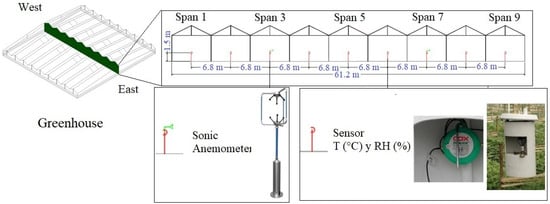
Figure 4.
Experimental distribution of temperature and air velocity recording sensors.
From the collected data during the experimental period, those corresponding to the hours 11:00 and 14:00 were selected (Table 2). These average data were established as initial simulation conditions for validation purposes. Once the convergence of each of these two simulations was achieved, the simulated temperature and air velocity data were obtained.
Table 2.
Initial simulation conditions for the validation scenarios.
The data from the simulations were compared with the experimental data through goodness-of-fit parameters, such as the root mean square error (RMSE) and the mean absolute percentage error (MAPE); these goodness-of-fit criteria are calculated according to Equations (7) and (8).
where n is the number of sampled data, and Dmi and Dsi are the measured and simulated values of temperature and air velocity, respectively. Once the validity of the CFD model was verified, the simulations of the scenarios established in Table 3 were performed. These simulation scenarios were set up using the above-mentioned local climatic variables and adjusting the airflow direction into each of the cardinal points (W, E, N, and S) in order to observe the effect of the wind direction on the renewal rates and the spatial distribution of the microclimate.
Table 3.
Entry conditions for the simulations of the evaluated scenarios.
Finally, in the post-processing stage, the spatial distribution curves and the numerical data of temperature and wind speed for each of the scenarios in a top view at a height of 1.5 m above ground level were obtained. This height was selected because it is generally the average height where cut flower crops are grown. Likewise, the renewal rates were calculated through the method of integration of the air flow rate that exits through each of the ventilation areas arranged in the greenhouse. This method has been successfully used in previous studies with similar approaches [2,22].
3. Results and Discussion
3.1. Validation of the CFD Model
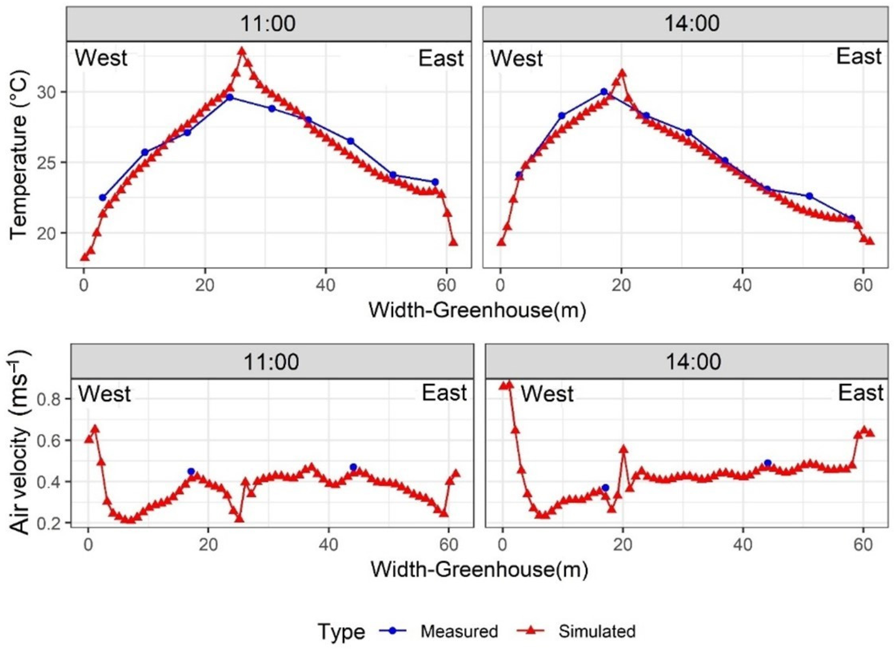
Figure 5 shows the graphs of the simulated data sets and the experimentally measured data. In general terms, it was found that the predictions made by the CFD model for temperature were within the trend reported experimentally, and the wind speed values coincide with the values predicted by the numerical model. Therefore, in qualitative terms, it can be mentioned that the model seems to have a high capacity to predict air flows and thermal distribution in the interior of the building.
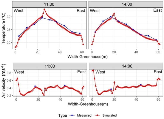
Figure 5.
Behavior of temperature and air velocity obtained during the validation process.
This validation was complemented with a numerical analysis in which for temperature, the RMSE and MAPE values were found to be 0.77 °C and 2.85% for hour 11, while for hour 14, they were 1.51 °C and 1.98%, respectively. Likewise, for air speed at hour 11, RMSE and MAPE values were 0.04 ms−1 and 7.63%, and 0.05 ms−1 and 9.78% were obtained for hour 14, respectively. These RMSE values are similar to those reported in other greenhouse natural ventilation studies [7,30]. Also, having MAPE values less than 10%, it can be concluded that the model has a highly accurate forecasting capability according to what is reported by Montaño Moreno et al. [31].
According to these results, the developed CFD model can be used to evaluate other ventilation configurations that can be implemented in this type of greenhouse. It is also possible for it to help in developing simulations in transient state, allowing simulations with the presence of the crop and its interaction with microclimate variables inside the greenhouse.
3.2. Airflow Patterns
3.2.1. Wind Perpendicular to Side Ventilation Areas
Figure 6 shows the simulated airflow patterns inside the greenhouse for scenarios S1 and S2 and for velocities V1 and V3. In the case of the S1V1 scenario, the air flow enters the greenhouse through the lateral ventilation area on the windward side at an average velocity of 0.68 ms−1; this flow moves transversely (E-W) to spans 4 and 5 and then slows down. There is also another air flow that enters the greenhouse in the opposite direction to the outside wind direction, entering at an average speed of 0.73 ms−1 through the upper ventilation area located on the leeward side and moves transversely (W-E) to the area located below spans 3 and 4.
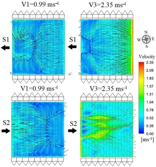
Figure 6.
Simulated airflow patterns for scenarios S1 (direction the wind is blowing: west; V1: 0.99 ms−1 and V3: 2.35 ms−1) and S2 (direction the wind is blowing: east; V1: 0.99 ms−1 and V3: 2.35 ms−1).
This entry of two flows in opposite directions leads to the generation of a short-circuit zone and recirculating air movement patterns right in the area where the flows meet and collide with each other. For scenario S1V1, it was also observed that the greenhouse air outflows were located over the ventilation areas arranged on the facades and in the leeward side ventilation area. This behavior of incoming air flows through ventilation areas arranged on the windward and leeward sides has been reported in other natural ventilation studies, such as the one developed by Molina-Aiz et al. [32] in a Spanish parral greenhouse.
For the S1V3 scenario, a similar pattern of behavior was observed with some marked differences, such as the leeward side airflow inflow velocity entering at an average velocity of 2.10 ms−1. This increase in air velocity is influenced by the increase in wind speed in the exterior. Likewise, it is observed that the short circuit and the recirculation loops reduce their sizes and are located closer to the leeward side. It is important to note that these scenarios where the wind comes from the east is the dominant climatic condition in the study region.
On the other hand, for the S2V1 scenario, an air flow is observed entering the greenhouse through the windward side ventilation area with an average velocity of 0.81 ms−1 and moving in a transverse direction (W-E) to just below the area below span 6. This flow subsequently collides with an incoming flow in the opposite direction and enters through the leeward ventilation area at an average velocity of 0.49 ms−1. This interaction between these two air flows again generates a short circuit region with little air movement.
Finally, for S2V3, there is a change of pattern in the movement of the air flows where it is quickly identified that the airflow entry through the leeward side disappears and, at the same time, the short circuit zone disappears. A higher velocity air flow is observed inside the greenhouse and a greater amount of air flow out of the interior of the structure through the ventilation areas of the facades and the leeward ventilation area.
3.2.2. Wind Perpendicular to the Ventilation Areas of the Facades
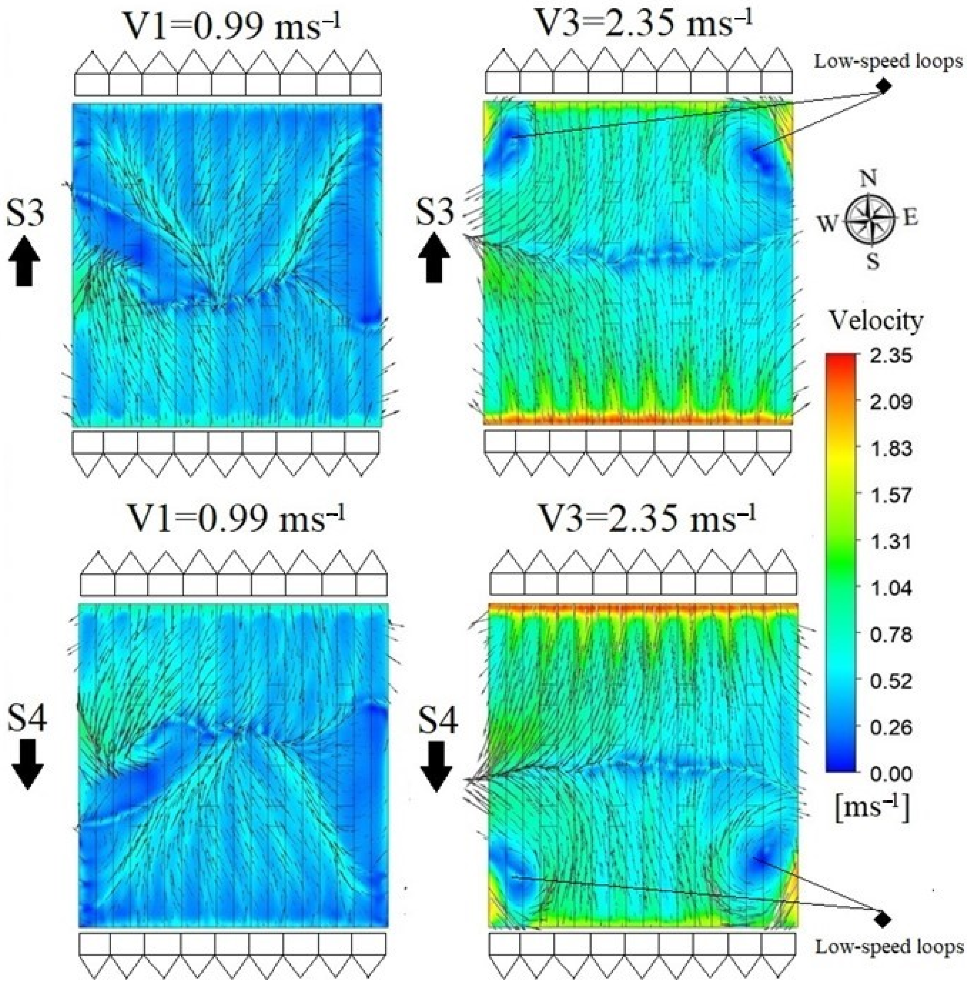
For S3V1, it was observed that airflows enter the greenhouse through the ventilation areas on the windward and leeward facades at an average velocity of 0.65 ms−1 and 0.59 ms−1, respectively (Figure 7). For these two air flows after entering the greenhouse, the first is directed longitudinally (S-N) until almost the middle zone of the greenhouse and collides with the flow that entered against the direction of the outside wind. This behavior generates again a zone of low air velocity, a zone that appears in the entire central transverse zone of the greenhouse and is distributed towards the sides and the leeward facade.
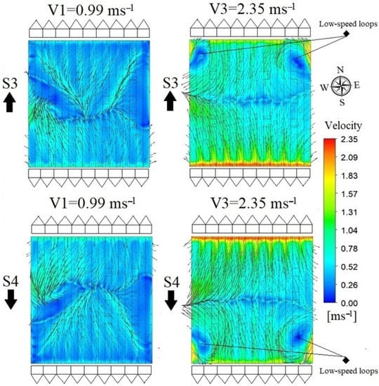
Figure 7.
Simulated airflow patterns for scenarios S3 (direction the wind is blowing: north; V1: 0.99 ms−1 and V3: 2.35 ms−1) and S4 (direction the wind is blowing: south; V1: 0.99 ms−1 and V3: 2.35 ms−1).
In the case of S3V3, an air flow enters the greenhouse through the ventilation of the windward facade at an average velocity of 2.12 ms−1 and then slows down as it moves longitudinally (S-N) until it reaches an average value of 0.98 ms−1. Likewise, the opposite direction flow (N-S) is observed again, although in this case, not through the entire window of the leeward façade since the perimeter edges of this region show the generation of two air flow movement loops with low velocity zones (Figure 7).
In these scenarios S3 V1 and V3, the greenhouse airflows exit through the ventilation areas on the sides of the structure. The airflow behaviors for S4V1 and S4V3 do not present very marked differences with the S3V1 and S3V3 scenarios; again, the areas of low velocity and airflow loops are observed in the central region, lateral, and perimeter corners of the leeward facade.
One last aspect to mention about the characteristics of the air flow patterns is the turbulent regime that is usually generated in some areas of the greenhouse region. These types of flows tend to occur even in conditions of low external wind speed (<2 ms−1) since, as demonstrated in the numerical study developed by Moghaddam [33], the formation of turbulent flow regimes depends on factors such as the shape of the structure, layout, and geometry of the ventilation areas. These same results had been previously verified experimentally in the work carried out by Lee et al. [19] and by McCartney et al. [34], who concluded that airflow turbulence plays a very relevant role in the natural ventilation process and on the spatial distribution of temperature inside the greenhouse.
3.2.3. Air Flow Velocity and Calculated Renewal Rates
For the quantitative analysis of the air velocity behavior for each of the simulated scenarios, a total of 49,381 data points were extracted from the plane analyzed in the previous sections. For each of the 12 scenarios, the mean velocity, standard deviation, and maximum and minimum air velocity values were calculated (Table 4). In the case of the scenarios simulated with V1 (0.99 ms−1), the values obtained ranged from a minimum of 0.36 ± 0.13 ms−1 for S2 to a maximum of 0.39 ± 0.15 ms−1 for S4, which represents a difference of 8.33% between S2 and S4.
Table 4.
Evaluated numerical parameters of the simulated airflow patterns.
In the case of V2 (1.75 ms−1), the mean air velocity oscillated between a minimum and maximum value presented in scenarios S1 and S2, respectively, with values of 0.45 ± 0.18 ms−1 and 0.59 ± 0.20 ms−1; therefore, in S4, the mean air velocity is 31.3% higher with respect to S2. For V3 (2.35 ms−1), the minimum value was 0.54 ± 0.23 ms−1 for S1 and a maximum value of 0.72 ± 0.28 ms−1 for S4, with this velocity being 33.3% higher than that of S1.
On the other hand, the minimum velocity values obtained for all scenarios ranged from 0.02 ms−1 to 0.09 ms−1, while the maximum velocity values ranged from 0.87 ms−1 to 2.12 ms−1. These values show that, in this type of structure, which does not have relevant ventilation areas in the roof region, the impact of outside wind conditions is quite heterogeneous, which in turn tends to lead to non-uniform spatial distributions of temperature inside the structure [26,35].
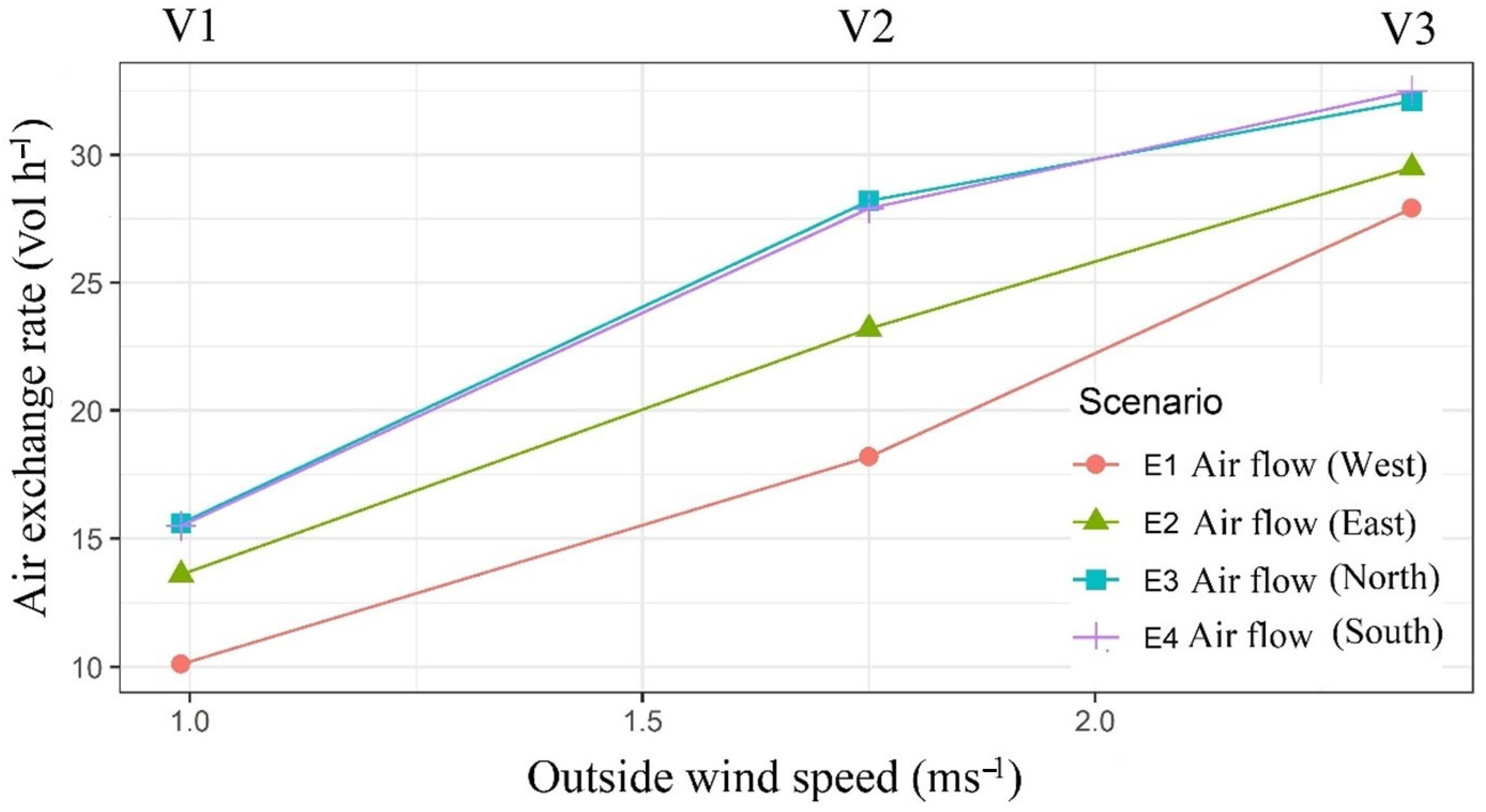
Figure 8 shows the air exchanges rates in volumes per hour for each of the simulated scenarios. For the four simulated scenarios S1–S4, it was observed that there is a direct relationship of the renewal rate value with the wind speed in the outdoor environment, which is in agreement with a large number of natural ventilation studies conducted in different types of greenhouses [7,30,36].
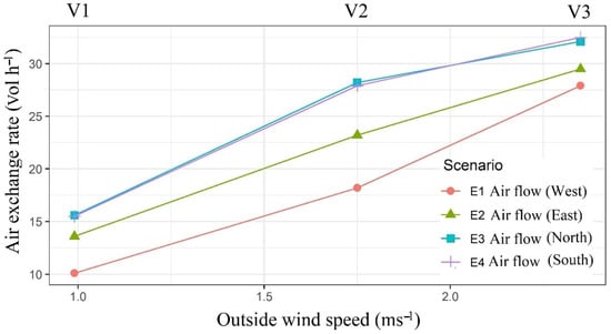
Figure 8.
Behavior of hourly renewal rates.
The renewal rate values were 10.1 Vol h−1 and 27.9 Vol h−1 for scenarios S1V1 and S1V3, respectively. For S2V1 and S2V3, these values were 13.6 Vol h−1 and 29.5 Vol h−1. For S3V1 and S3V3 the renewal rates were 15.6 Vol h−1 and 32.1 Vol h−1, respectively. Finally, for S4, the values were 15.5 Vol h−1 and 32.5 Vol h−1 for V1 and V3, respectively.
It should also be noted that these values found based on the behavior of the wind speed characteristic of the study region did not allow us to obtain a value of adequate air exchange for passive type greenhouse. The index at least should be at least equal to 40 air exchange per hour and ideally reach 60 volumes per hour [9,37].
3.3. Spatial Distribution of Temperature
The spatial behavior of temperature for all simulated scenarios in a plan view at a height above ground level of 1.5 m is presented in Figure 9. In general terms, it is possible to identify the qualitative distribution of temperature showing a highly heterogeneous behavior, while thermal differentials for the same moment can exceed 10.0 °C. These values exceed the thermal differentials reported in experimental studies in other types of passive greenhouses used in the Colombian ornamental sector, similar to the studies developed by Villagrán and Bojacá [6] and Villagrán and Bojacá [38].
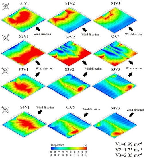
Figure 9.
Spatial behavior of temperature for 12 simulated scenarios; S1 (direction the wind is blowing: west; V1: 0.99 ms−1; V2: 1.75 ms−1 and V3: 2.35 ms−1); S2 (direction the wind is blowing: east; V1: 0.99 ms−1; V2: 1.75 ms−1 and V3: 2.35 ms−1); S3 (direction the wind is blowing: north; V1: 0.99 ms−1; V2: 1.75 ms−1 and V3: 2.35 ms−1); and S4 (direction the wind is blowing: south; V1: 0.99 ms−1; V2: 1.75 ms−1 and V3: 2.35 ms−1).
For scenario S1, the highest temperature zone is located in the central zone of the greenhouse and moves towards the leeward side, while the lowest temperature zones are located on the windward side and in the middle region of the leeward side where the air flows enter the greenhouse (Figure 9). In the case of S2, it is observed that for V1, the high-temperature region is located along the entire longitudinal direction of the greenhouse covering the area between the span 4 and the leeward side. For V2 and V3, there are areas with the lowest temperature, corresponding to the areas where air flows enter the greenhouse through the upper lateral ventilation of the leeward wall. On the other hand, for these scenarios, the highest-temperature zones are now located on the inner edges of the facades and on the corners of the windward side region.
For scenarios S3 and S4, similar behaviors were observed, where the lowest temperature occurred just above the regions where the air flows enter, which, in these cases, is through the regions of the facades. It is also observed that the regions of higher temperature are located on the central transverse region of the greenhouse and are distributed towards the regions of the facade in greater and lesser areas depending on the external wind speed.
For the quantitative analysis of temperature behavior, the data was qualitatively analyzed based on the mean temperature (Tm), the maximum temperature (Tmax), the minimum temperature (Tmin), the thermal differential inside the greenhouse (ΔTinside), and the thermal differential between the mean inside temperature and the simulated outside temperature (ΔT), calculations that are summarized in the Table 5.
Table 5.
Quantitative parameters of the simulated temperature behavior.
The values of Tm ranged for V1 between 25.9 ± 3.0 °C and 27.3 ± 4.0 °C for S4 and S2, respectively. This range is between 23.3 ± 2.7 °C and 25.7 ± 4.1 °C for the S4 and S2 scenarios of V2, while for V3, the Tm is ranged between 22.6 ± 2.6 °C and 24.2 ± 3.4 °C in S4 and S2, respectively. On the other hand, Tmin values obtained in all scenarios have values below 19.0 °C. While Tmax exceeded 32.0 °C in all scenarios in some specific regions, they reached an extreme value of 37.2 °C in S2V1.
Regarding climatic heterogeneity, it can be observed some values are considerably high, allowing quantitative identifications of the greenhouses with highly heterogeneous behavior of ΔTinside values ranged between 13.1 °C for S4V3 and 18.6 °C for S2V1. These values are well above the recommendation established for a greenhouse where, as far as possible, the temperature differentials in the indoor environment should not exceed 2 °C [39].
Finally, it is important to mention that these results reaffirm that, in the traditional Colombian greenhouse, there is a highly heterogeneous thermal behavior associated with the type of structure, the ventilation configuration, and the low renovation rates generated for the climatic conditions of the study region. This thermal heterogeneity is one of the aspects that has been mostly investigated in the recent years, as it is a factor that generates negative consequences on the production of cut flowers, since temperature affects processes such as transpiration and translocation of nutrients in plants; therefore, under this type of behavior, it is very common to obtain non-uniform productions [10].
Likewise, these differential temperature behaviors tend to produce flowers with low-commercial-quality parameters, such as short stem lengths, flower heads with non-uniform and curved colors, and flower stems affected by browning. Finally, it is important to mention that the maximum extreme temperature values presented in the greenhouse far exceed the recommended values for the production of the main cut flowers of commercial interest, such as roses and carnations, where average daytime temperatures should ideally be close to 25 °C or not to exceed this value as far as possible [29].
4. Conclusions
In this research, an experimentally validated 3D CFD model was used to simulate the behavior of air flows inside a traditional Colombian greenhouse under the conditions of four wind directions (S1, S2, S3, and S4) and four wind speeds (V1, V2, V3, and V4) in the outdoor environment. The results have shown that wind should be considered as another input to be managed for the benefit of micro-climatic comfort within passive greenhouse used for cutting flower production.
The three-dimensional simulations carried out allowed us to identify that, in the inside of the traditional Colombian greenhouse, inadequate final conditions are generated with a heterogeneous spatial distribution with the presence of factors that depend directly on wind direction and speed. Therefore, it was found that for wind speeds V1 (0.99 ms−1), the generated heat spots are in an approximate area of up to 50% of the cultivated area inside the greenhouse and with a temperature value for S2V1 of up to 37.2 °C. On the contrary, for the scenarios with V3 velocities (2.35 ms−1), it was observed that the areas with heat spots are reduced inside the greenhouse to an approximate area of less than 20% of the total covered area, and at the same time, the highest temperature value was 34.4 °C for S2V3; it should be noted that these temperature values are not appropriate for cut flower production.
This study also reaffirmed the deficiencies in terms of ventilation in the traditional Colombian greenhouse; for the typical conditions of the study region, the air exchanges rates in all scenarios were below the minimum recommended value of 40 air exchanges per hour. This behavior of the air renewal rate promotes the generation of highly heterogeneous thermal distribution conditions in the space and with inadequate values for the production of cut flowers during the main hours of the daytime period.
Finally, this work establishes the technical and numerical simulation bases that will allow future studies to propose more realistic analyses where some type of crops can be included, be it ornamental, horticultural, or medicinal, since locally this type of greenhouse is the most used in these three production systems. This type of simulations can be developed in order to analyze some additional microclimate variables involved in crop growth dynamics, such as humidity and CO2. Additionally, based on the results obtained in this research, a microclimate optimization study can be carried out in this greenhouse design, an optimization that can be proposed by adding a ventilation area in the greenhouse roof region and a greater overall height of the greenhouse, structural variables that can provide greater air exchange and more uniform microclimate conditions.
Author Contributions
Conceptualization, E.V., M.A. and J.F.-V.; methodology, E.V., C.B., J.F.-V. and M.A.; software, E.V.; validation, E.V. and C.B.; investigation, E.V. and C.B.; writing—original draft preparation, E.V., C.B., J.F.-V. and M.A.; writing—review and editing, E.V., C.B., J.F.-V. and M.A. All authors have read and agreed to the published version of the manuscript.
Funding
The present study was funded by the Sistema General de Regalías and the Gobernacion de Cundinamarca through the project “Fortalecimiento de la competitividad del sector floricultor colombiano mediante el uso de ciencia, tecnología e innovación aplicadas en el departamento de Cundinamarca” code: BPIN2013000100217.
Institutional Review Board Statement
Not applicable.
Informed Consent Statement
Not applicable.
Data Availability Statement
Not applicable.
Conflicts of Interest
The authors declare no conflict of interest.
References
- Ghani, S.; El-Bialy, M.; Bakochristou, F.; Mohamed Rashwan, M.; Mohamed Abdelhalim, A.; Mohammad Ismail, S.; Ben, P. Experimental and numerical investigation of the thermal performance of evaporative cooled greenhouses in hot and arid climates. Sci. Technol. Built Environ. 2020, 26, 141–160. [Google Scholar] [CrossRef] [Green Version]
- Senhaji, A.; Mouqallid, M.; Majdoubi, H. CFD Assisted Study of Multi-Chapels Greenhouse Vents Openings Effect on Inside Airflow Circulation and Microclimate Patterns. Open J. Fluid Dyn. 2019, 9, 119–139. [Google Scholar] [CrossRef] [Green Version]
- Akrami, M.; Javadi, A.A.; Hassanein, M.J.; Farmani, R.; Dibaj, M.; Tabor, G.R.; Negm, A. Study of the effects of vent configuration on mono-span greenhouse ventilation using computational fluid dynamics. Sustainability 2020, 12, 986. [Google Scholar] [CrossRef] [Green Version]
- Villagrán, E.; Leon, R.; Rodriguez, A.; Jaramillo, J. 3D numerical analysis of the natural ventilation behavior in a Colombian greenhouse established in warm climate conditions. Sustainability 2020, 12, 8101. [Google Scholar] [CrossRef]
- Akrami, M.; Mutlum, C.D.; Javadi, A.A.; Salah, A.H.; Fath, H.; Dibaj, M.; Farmani, R.; Mohammed, R.H.; Negm, A. Analysis of inlet configurations on the microclimate conditions of a novel standalone agricultural greenhouse for Egypt using computational fluid dynamics. Sustainability 2021, 13, 1446. [Google Scholar] [CrossRef]
- Villagrán, E.; Bojacá, C. Experimental evaluation of the thermal and hygrometric behavior of a Colombian greenhouse used for the production of roses (Rosa spp.). Ornam. Hortic. 2020, 26, 205–219. [Google Scholar] [CrossRef]
- Villagrán, E.A.; Romero, E.J.B.; Bojacá, C.R. Transient CFD analysis of the natural ventilation of three types of greenhouses used for agricultural production in a tropical mountain climate. Biosyst. Eng. 2019, 188, 288–304. [Google Scholar] [CrossRef]
- Diaz, D.C.; Bojacá, C.R.; Schrevens, E. Modeling the suitability of the traditional plastic greenhouse for tomato production across Colombian regions. Acta Hortic. 2018, 1205, 857–864. [Google Scholar] [CrossRef]
- Reynafarje, X.; Villagrán, E.A.; Bojacá, C.R.; Gil, R.; Schrevens, E. Simulation and validation of the airflow inside a naturally ventilated greenhouse designed for tropical conditions. Acta Hortic. 2020, 1271, 55–62. [Google Scholar] [CrossRef]
- Taki, M.; Ajabshirchi, Y.; Ranjbar, S.F.; Rohani, A.; Matloobi, M. Modeling and experimental validation of heat transfer and energy consumption in an innovative greenhouse structure. Inf. Process. Agric. 2016, 3, 157–174. [Google Scholar] [CrossRef] [Green Version]
- In, B.C.; Lim, J.H. Potential vase life of cut roses: Seasonal variation and relationships with growth conditions, phenotypes, and gene expressions. Postharvest Biol. Technol. 2018, 135, 93–103. [Google Scholar] [CrossRef]
- Valera, D.L.; Molina-Aiz, F.D.; Moreno, M.A.; López, A.; Marın, P. Ventilation surface area: Key to modify morphology, quality and photosynthetic activity of tomato crops in Mediterranean greenhouses. Acta Hortic. 2020, 1296, 185–192. [Google Scholar] [CrossRef]
- McCartney, L.; Lefsrud, M.G. Field trials of the Natural Ventilation Augmented Cooling (NVAC) greenhouse. Biosyst. Eng. 2018, 174, 159–172. [Google Scholar] [CrossRef]
- Akrami, M.; Salah, A.H.; Javadi, A.A.; Fath, H.E.; Hassanein, M.J.; Farmani, R.; Negm, A. Towards a Sustainable Greenhouse: Review of Trends and Emerging Practices in Analysing Greenhouse Ventilation Requirements to Sustain Maximum Agricultural Yield. Sustainability 2020, 12, 2794. [Google Scholar] [CrossRef] [Green Version]
- Cortés-Rojas, M.H.; Mesa-Torres, P.A.; Grijalba-Rativa, C.M.; Pérez-Trujillo, M.M. Yield and fruit quality of the blueberry cultivars Biloxi and Sharpblue in Guasca, Colombia. Agron. Colomb. 2016, 34, 33–41. [Google Scholar] [CrossRef]
- Medina Campos, L.; Hinestrosa, L.; Perea, M.; Ortega, J.; Ballén Zamora, S.A. Aproximación a la Zonificación Bioclimática de Cundinamarca. 2018, p. 192. Available online: https://www.researchgate.net/publication/330761489_Aproximacion_a_la_Zonificacion_Bioclimatica_de_Cundinamarca (accessed on 3 January 2021).
- Li, H.; Li, Y.; Yue, X.; Liu, X.; Tian, S.; Li, T. Evaluation of airflow pattern and thermal behavior of the arched greenhouses with designed roof ventilation scenarios using CFD simulation. PLoS ONE 2020, 15, e0239851. [Google Scholar] [CrossRef]
- Villagrán, E.; Ramirez, R.; Rodriguez, A.; Pacheco, R.L.; Jaramillo, J. Simulation of the thermal and aerodynamic behavior of an established screenhouse under warm tropical climate conditions: A numerical approach. Int. J. Sustain. Dev. Plan 2020, 15, 487–499. [Google Scholar] [CrossRef]
- Lee, S.Y.; Lee, I.B.; Kim, R.W. Evaluation of wind-driven natural ventilation of single-span greenhouses built on reclaimed coastal land. Biosyst. Eng. 2018, 171, 120–142. [Google Scholar] [CrossRef]
- Román-Roldán, N.I.; López-Ortiz, A.; Ituna-Yudonago, J.F.; García-Valladares, O.; Pilatowsky-Figueroa, I. Computational fluid dynamics analysis of heat transfer in a greenhouse solar dryer “chapel-type” coupled to an air solar heating system. Energy Sci. Eng. 2019, 7, 1123–1139. [Google Scholar] [CrossRef]
- Benni, S.; Santolini, E.; Barbaresi, A.; Torreggiani, D.; Tassinari, P. Calibration and comparison of different CFD approaches for airflow analysis in a glass greenhouse. J. Agric. Eng. 2017, 48, 49–52. [Google Scholar] [CrossRef] [Green Version]
- Hong, S.W.; Lee, I.B.; Hwang, H.S.; Seo, I.H.; Bitog, J.P.; Yoo, J.I. Numerical simulation of ventilation efficiencies of naturally ventilated multi-span greenhouse in Korea. Trans. ASABE 2008, 51, 1417–1432. [Google Scholar] [CrossRef]
- Bournet, P.E.; Morille, B.; Migeon, C. CFD prediction of the daytime climate evolution inside a greenhouse taking account of the crop interaction, sun path and ground conduction. Acta Hortic. 2017, 1170, 61–70. [Google Scholar] [CrossRef]
- Flores-Velázquez, J.; Rojano-Aguilar, A.V.; Rojas-Rishor, A.; Ojeda-Bustamante, W. Energy exchange by convection in a closed greenhouse a pipe heating system: A CFD analysis. Am. Soc. Agric. Biol. Eng. Annu. Int. Meet. 2015. [Google Scholar] [CrossRef]
- Shao, H.B.; Chu, L.Y.; Jaleel, C.A.; Zhao, C.X. Water-deficit stress-induced anatomical changes in higher plants. Comptes Rendus Biol. 2008, 331, 215–225. [Google Scholar] [CrossRef]
- Villagrán, E.A.; Bojacá, C.R. Effects of surrounding objects on the thermal performance of passively ventilated greenhouses. J. Agric. Eng. 2019, 50, 20–27. [Google Scholar] [CrossRef]
- Kuroyanagi, T.; Iyonaga, M.; Sunada, K.; Ohnishi, N.; Hashimoto, K. Development of CFD model of a greenhouse with water-sprinkling roof. Acta. Hortic. 2009, 893, 613–620. [Google Scholar] [CrossRef]
- Tadj, N.; Bartzanas, T.; Fidaros, D.; Draoui, B.; Kittas, C. Influence of heating system on greenhouse microclimate distribution. Trans. ASABE 2010, 53, 225–238. [Google Scholar] [CrossRef]
- Villagrán, E.A.; Bojacá, C.R. Study of natural ventilation in a Gothic multi-tunnel greenhouse designed to produce rose (Rosa spp.) in the high-Andean tropic. Ornam. Hortic. 2019, 25, 133–143. [Google Scholar] [CrossRef] [Green Version]
- Mesmoudi, K.; Meguallati, K.H.; Bournet, P.E. Effect of the greenhouse design on the thermal behavior and microclimate distribution in greenhouses installed under semi-arid climate. Heat Transf. Asian Res. 2017, 46, 1294–1311. [Google Scholar] [CrossRef]
- Montaño Moreno, J.J.; Palmer Pol, A.; Sesé Abad, A.; Cajal Blasco, B. Using the R-MAPE index as a resistant measure of forecast accuracy. Psicothema 2013. [Google Scholar] [CrossRef]
- Molina-Aiz, F.D.; Valera, D.L.; Pena, A.A.; Alvarez, A.J.; Gil, J.A. Analysis of the effect of rollup vent arrangement and wind speed on Almería-type greenhouse ventilation performance using computational fluid dynamics. Acta Hortic. 2006, 719, 173–180. [Google Scholar] [CrossRef]
- Moghaddam, J.J. The effect of turbulence on natural ventilation of a proposed octagonal greenhouse in a transient flow. Int. J. Environ. Sci. Technol. 2020, 1–16. [Google Scholar] [CrossRef]
- McCartney, L.; Orsat, V.; Lefsrud, M.G. An experimental study of the cooling performance and airflow patterns in a model Natural Ventilation Augmented Cooling (NVAC) greenhouse. Biosyst. Eng. 2018, 174, 173–189. [Google Scholar] [CrossRef]
- Espinoza, K.; López, A.; Valera, D.L.; Molina-Aiz, F.D.; Torres, J.A.; Pena, A. Effects of ventilator configuration on the flow pattern of a naturally-ventilated three-span Mediterranean greenhouse. Biosyst. Eng. 2017, 164, 13–30. [Google Scholar] [CrossRef]
- Bournet, P.E.; Boulard, T. Effect of ventilator configuration on the distributed climate of greenhouses: A review of experimental and CFD studies. Comput. Electron. Agric. 2010, 74, 195–217. [Google Scholar] [CrossRef]
- Romero-Gómez, P.; Choi, C.Y.; Lopez-Cruz, I.L. Enhancement of the greenhouse air ventilation rate under climate conditions of central méxico mejora de las tasas de ventilación de invernaderos bajo condiciones climáticas del centro de México. Agrociencia 2010, 44, 1–15. Available online: http://www.scielo.org.mx/pdf/agro/v44n1/v44n1a1.pdf (accessed on 4 October 2020).
- Villagran Munar, E.A.; Bojaca Aldana, C.R.; Bahamon Rojas, N.A. Determinacion del comportamiento térmico de un invernadero espacial colombiano mediante dinámica de fluidos computacional. Rev. UDCA Act. Div. Cient. 2018, 21, 415–426. [Google Scholar] [CrossRef]
- Zorzeto, T.Q.; Leal, P.A.M.; Nunes, E.F.; de Araújo, H.F. Homogeneity of temperature and relative humidity of air in greenhouse. In International Proceedings of Chemical, Biological and Environmental Engineering (IPCBEE); IACSIT Press: Singapore, 2014; Volume 79, pp. 25–29. [Google Scholar] [CrossRef]


Publisher’s Note: MDPI stays neutral with regard to jurisdictional claims in published maps and institutional affiliations. |
© 2021 by the authors. Licensee MDPI, Basel, Switzerland. This article is an open access article distributed under the terms and conditions of the Creative Commons Attribution (CC BY) license (https://creativecommons.org/licenses/by/4.0/).