5.1. Soil Salinity and the Electrical Conductivity of the Soil
The electrical conductivity (EC) of a soil: water extract is commonly used to estimate soil salinity. This was the method used in the report. The US Salinity Laboratory Staff [
38] established the EC of the extract of a saturated paste of soils (ECe) to evaluate the effect of soil salinity on plant growth.
The US Salinity Laboratory Staff [
38] also recommends EC1:5, i.e., the EC for a soil to water ratio of 1:5, to determine the change in salinity with time or treatment. The two-fixed dilutions approach [
39] can help to refine the assessments of the stock of soluble salts in the soil. Nowadays, other methods can speed up the direct measurements of soil salinity by using modern sensors [
40,
41]. Advances in both instrumentation and methods can yield a wealth of new soil salinity data, whose comparison with heritage data will help in understanding and modeling the trend in salinity, a prime factor to the sustainability of agriculture in irrigated lands. The sustainable management of water and soils is a key strategy in the European Green Deal, supporting a whole host of EU policies in a variety of areas, from agriculture and food security to environmental protection.
The IRYDA report [
32,
33] uses ECe to classify the soil profiles studied and to express the tolerance of crops to soil salinity. By contrast, the report uses EC1:5 to depict the soil salinity of the entire irrigation district. The IRYDA report [
33], on pages 157–161, shows the major ions and several parameters of the irrigation water by monthly samplings in four consecutive months from May to July of 1975 at the start of the Monegros Canal. The mean electrical conductivity of the water was 0.38 dS m
−1, ranging from 0.33 dS m
−1 to 0.41 dS m
−1, the mean Na
+ content was 6.7 dS m
−1, and the sodium-adsorption-ratio (SAR) ranged from 0.5 to 0.6 (mmol L
−1)
0.5.
5.2. Soil Analysis Methods in 1975
The IRYDA laboratory in Madrid—closed in 1992—analyzed the 85 soil samples taken in the 24 soil profiles in pits described on pages 31 to 132 in Annex 3 of IRYDA [
33]. The determinations were particle size distribution, organic matter, pH, calcium carbonate, and soluble chloride. This lab also prepared the saturation extracts of these samples, determining their electrical conductivity (ECe, dS m
−1), and the content in meq L
−1 of (Ca
2+ + Mg
2+) and Na
+. We disregard here the determination of “soluble Cl
−” because the report does not provide the extraction method, and our consultation on 22 November 2001 with the last manager of the IRYDA lab was inconclusive. The lab of the private company “Unión Explosivos Río Tinto” determined the electrical conductivity of the 1:5 soil to water extracts by weight (EC1:5, dS m
−1) and the pH in water at a 1:1 soil to water dilution (pH1:1) for the samples of the augerings.
The IRYDA report [
2] on pages 6-9 describes the analytical methods. We do not present the texture determinations because the report refers to “the Kilmer method”—perhaps [
42]—with unspecified variations. Annex 3 [
33] describes the 24 soil profiles classified at the Subgroup level, as per the then-available version of Soil Taxonomy [
43], and provides the percent of the particle-size separates. By contrast, the auger samples (Annex 4) only use Spanish terms to describe the texture, which are somewhat different from the USDA standard terms. At any rate, since the textures are time invariant, the data in the report might be useful for verification purposes in possible future destructive samplings. Similar considerations apply for the pH determinations.
The statistics of analytical data in this paper do not include the means of pH and SAR, because the non-additivity of these parameters make their means chemically unsound. Thus, we only present the median as a measure of centrality for pH and SAR.
5.4. The Stock of Soluble Salts in the Soil
Annex 4 of the report [
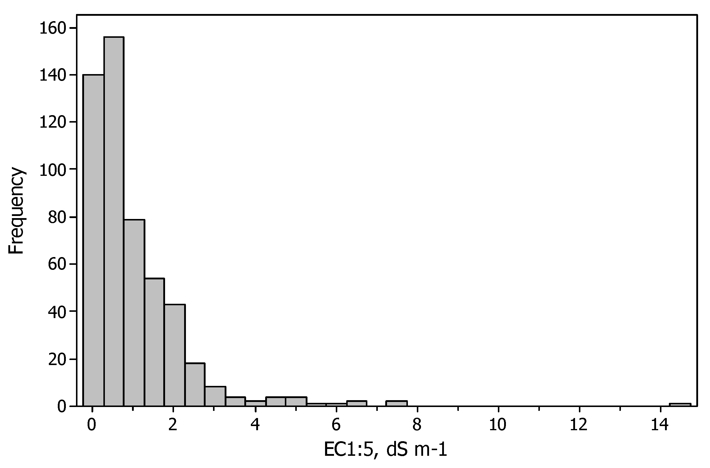
33] contains the analytical data of 519 soil samples taken with auger from 183 sites. The augerings are numbered in the report from 1 to 197, with 14 gaps or missing numbers: 13, 29, 31, 48, 125, 145–152, and 183. The depth of the augerings ranged from 20 cm to 230 cm, with a mean of 108.4 cm and a median of 110 cm. Site no. 96, described in the report as “surficial”, had a disparately high EC1:5 of 14.5 dS m
−1 (
Figure 3), suggesting that this sample contained an efflorescence. For further computing, we assign to this sample a depth of 0–1 cm.
The EC1:5 of the 519 samples ranged from 0.11 dS m
−1 to 14.5 dS m
−1 with a mean of 0.99 dS m
−1 and a median of 0.57 dS m
−1; the mean of EC1:5 weighted by the sample depth interval was 0.95 dS m
−1. The values of EC1:5 for the auger samples and the numbers assigned by us to each sample are available in the file “Augerings 1975 Monegros.docx” [
44], The right-skewed distribution (
Figure 3) is typical for the EC of soils.
We assess the stock of salts in the district from the 519 determinations of EC1:5 listed in pages 135–149 of Annex 4 [
33] and collected in the file “Augerings 1975 Monegros.docx” [
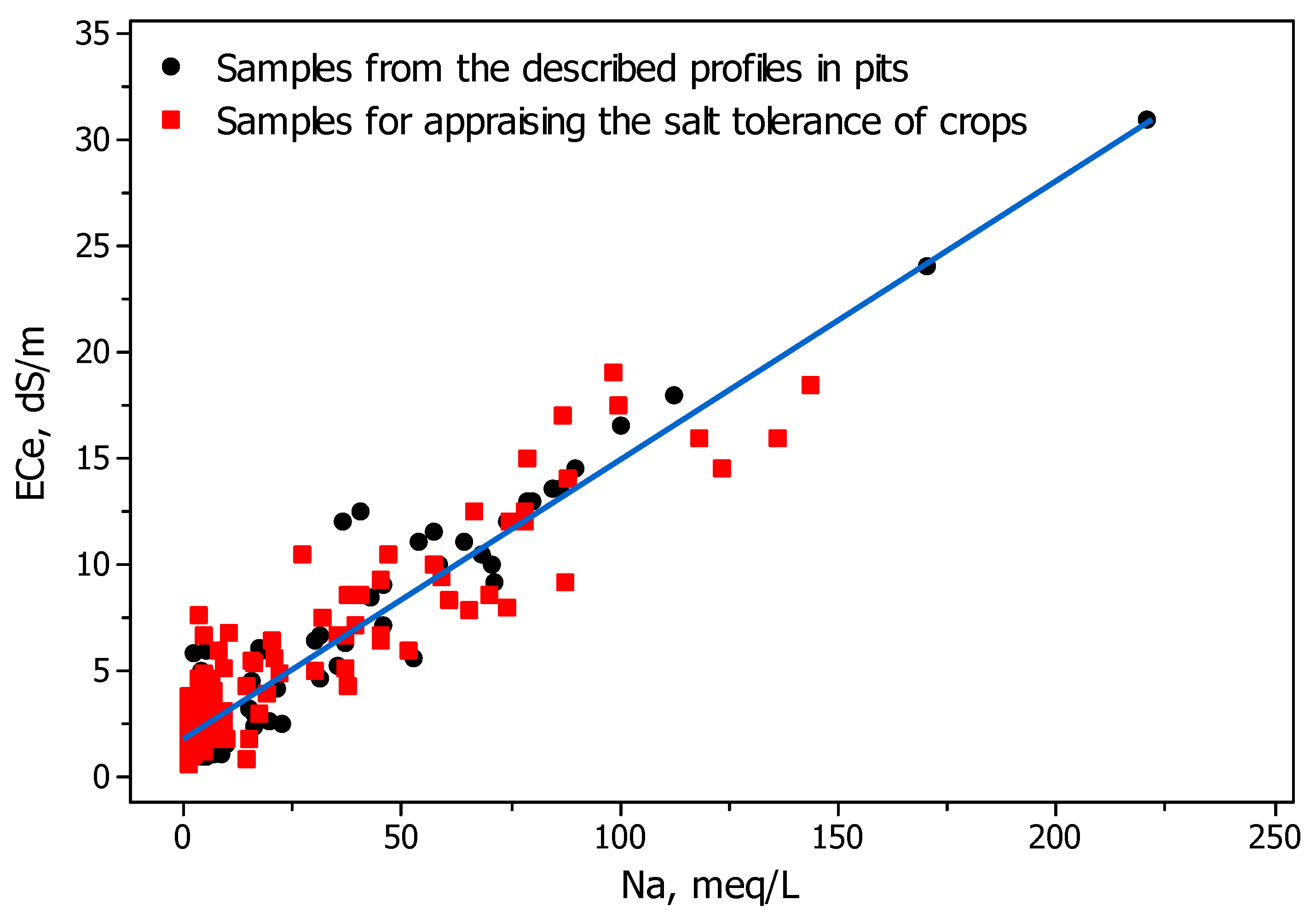
44]. In this table, we disregard ECe, despite the coefficient of determination R
2 = 89.6% of the ECe regression over EC1:5, because the ECe values were not determined in the lab, but estimated from EC1:5 by means of separate regressions for samples grouped by their texture. On pages 151 and 152 of [
33], the report has two graphs, both with a poor adjustment, for different soil textures. Our scatterplot of ECe vs. EC1:5 for the 519 soil samples (not shown here) also evidences independent estimations by texture. Moreover, these estimates did not consider the presence of gypsum in some areas of the district, a circumstance that modifies the relationship ECe/EC1:5 [
38,
39,
45]. Furthermore, ECe was conceived to express the salt stress on plants, while EC1:5 is a better proxy for total salt content in the soil [
38,
39]. A non-trivial advantage of EC1:5 is the simplicity of the method, which enhances the reliability of the determinations and their repeatability even in field-based laboratories. The Annex also contains the “ESP intervals”, but we disregard this non-numerical information because ESP is supposedly an estimate from SAR, whose values are not provided in the report.
The above-mentioned file “Augerings 1975 Monegros.docx” [
44] can be used to easily prepare tables of EC1:5 for customized depths. This kind of table would be necessary to calculate the stock of salts to arbitrary depths, as well as to match with new augering campaigns or with prospections using fixed-penetration instruments.
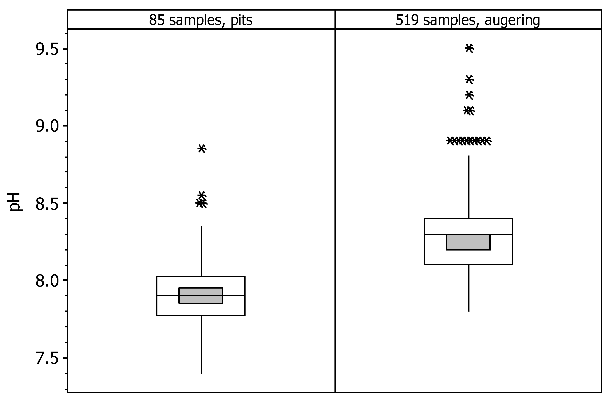
The pH in the 519 1:1 soil to water auger samples are shown in the file “Augerings 1975 Monegros.docx” [
44], and in
Figure 4. The pH ranges from 7.8 to 9.5, with a median of 8.30. The values of pH1:1 are hardly comparable with the pH of the 85 samples from the 24 soil profiles studied, whose dilution ratio was not ascertained, as noted at
Table 3. We could assume a dilution of 1:2.5, as per the official Spanish methods for soil analyses [
46], but the distributions of the two sets of pH determinations are significantly different (
Figure 4) and the pH values are higher in the auger samples. By contrast, the pH of the auger samples, as determined at a 1:1 dilution, would be expected to be lower than that of the pits if their dilution were 1:2.5 [
47,
48]. Due to these circumstances and to the limited value of pH for temporal comparisons of the stock of salts in the soil, we do not give further consideration in this article to the pH values.
5.5. Location of the Soil Sampling Sites
The soil surveyors had 278 contact prints of 23 × 23 cm from the photogrammetric flight CETFA 57/72 performed in May 1972. The prints, marked with colored wax crayon by the soil surveyors, had a scale of 1:10,000. The scans in PDF format of the 176 contact prints, which have marks from the surveyors for locating the sampling sites, plus the flight diagram are recorded in the file “Marked contacts CETFA Monegros1972 and diagram.zip” [
44]. Most of the wax marks are crosses and dots indicating the sampling sites, but there are also other features, like village names and isolated boundary lines for some plots. The crayon strokes are about 2 mm thick, i.e., ≈20 m on the ground. This precision is allowable for the sampling sites since most of the smaller plots in the photographs are about 20 m wide. Moreover, a higher precision is not necessary, and it might even be undesirable, for repeated destructive paired samplings due to the localization paradox [
49].
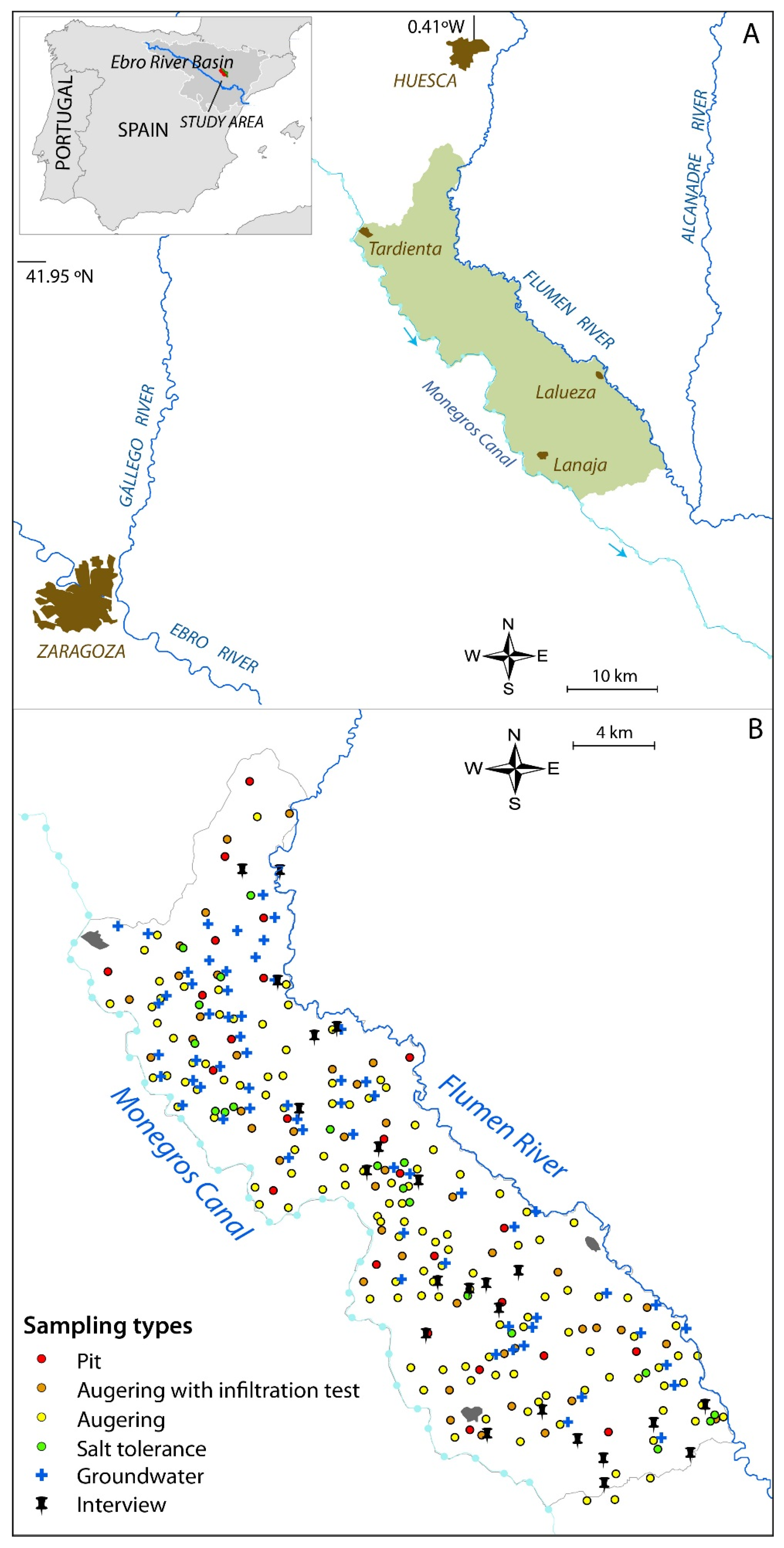
We established the UTM coordinates ETRS89 of the sites sampled in 1972 based on their representation in Map 2, yielding
Figure 1B. The document used to georeference the sampling sites was the historic black and white orthophotographs of the OLISTAT Oleícola flight (1997–1998, scale 1:40,000, pixel size 1 m), freely available at the National Center of Geographic Information (CNIG) (
https://centrodedescargas.cnig.es/CentroDescargas/catalogo.do?Serie=02211, accessed on 22 December 2021). The 34 control points between Map 2 and the OLISTAT mosaic allowed a mean error of 85 m. The OLISTAT images have an acceptable quality and, since they were taken before the general shift to pressurized irrigation, they still allow for most of the plots sampled in 1972 to be easily identified. The entire irrigated district falls within the 100 km
2 square 30T YM. The UTM coordinates obtained for the soil sampling sites are available at the file “Coordinates 1975 Monegros.docx” [
44].
The incomplete matches between (i) sampling sites shown in Map 2 in [
33], (ii) the list of sites, and (iii) the points marked on the contact prints used by the surveyors, makes it impossible to associate a few of the sample points with their analytical data, and vice versa.


