Double-DQN-Based Path-Tracking Control Algorithm for Orchard Traction Spraying Robot

Abstract

The precise path-tracking control of tractors and trailers is the key to realizing agricultural automation. In order to improve the path-tracking control accuracy and driving stability of orchard traction spraying robots, this study proposed a navigation path-tracking control algorithm based on Double Deep Q-Network (Double DQN). Drawing on the driver’s driving experience and referring to the principle of radar scanning and the principle of image recognition, a virtual radar model was constructed to generate a virtual radar map. The virtual radar map was used to describe the position relationship between the traction spraying robot and the planned path. Combined with the deep reinforcement learning method, all possible robot driving actions under the current virtual radar map were scored, and the best driving action was selected as the output of the network. In this study, a path-tracking algorithm was self-developed with a deep Q-network trained by driving the traction spraying robot in a simulated virtual environment. The algorithm was tested in both simulations and in a field to follow a typical ‘U’-shaped path. The simulation results showed that the proposed algorithm was able to achieve accurate path-tracking control of the spraying trailer. The field tests showed that when the vehicle speed was 0.36 m/s and 0.75 m/s, the maximum lateral deviation of the algorithm was 0.233 m and 0.266 m, the average lateral deviation was 0.071 m and 0.076 m, and the standard deviation was 0.051 m and 0.057 m, respectively. Compared with the algorithm based on the virtual radar model, the maximum lateral deviation was reduced by 56.37% and 51.54%, the average lateral deviation was reduced by 7.8% and 5.0%, and the standard deviation was reduced by 20.31% and 8.1%, respectively. The results showed that the Double-DQN-based navigation path-tracking control algorithm for the traction spraying robot in the orchard had higher path-tracking accuracy and driving stability, which could meet the actual operational requirements of traditional orchards.

1. Introduction

China’s orchards are currently divided into standard orchards and traditional orchards. The traditional orchards’ planting area accounts for about 75% of all orchard area [1]. Pest and disease control work is an important part of orchard fruit tree management. With changes in season and climate, 8~15 spraying times per year occur, and this workload accounts for about 30% of the whole fruit tree management workload [2,3]. However, traditional orchards are densely planted, and their access roads are low and narrow, which makes it difficult for ordinary agricultural machinery to enter and operate [4]. Because the traction structure can effectively reduce the height of the whole machine to adapt to a low-channel working environment, it is widely used.

The goal of automatic navigation or guidance of agricultural machinery is to control the trajectory of the vehicle so that it maintains a constant distance from the adjacent driving line. Most scholars at home and abroad are committed to keeping the distance between the tractor and the planned path constant. In fact, different from self-propelled rice transplanters, fertilizer applicators and seeders, the goal of traction agricultural machinery navigation should be to maintain the operating points in the machine, such as the plough knife in the seeder, the flat shovel of the grader or the spraying trailer in the traction spraying robot, and keep a constant distance from the planned path. At present, domestic and foreign scholars have little research on the path-tracking control of the orchard traction spraying robot navigation, and the tractors are mainly wheeled tractors. As the steering principles of tracked vehicles and wheeled vehicles are different, the path-tracking algorithms of wheeled vehicles are difficult to apply directly to tracked vehicles [5,6]. However, accurate path tracking is the key for spraying robots to achieve precise spraying of agricultural crops [7]. Especially when working on a curved road, the driving track of a trailer is different from that of the tractor. Navigating the tractor alone can result in path gaps and overlaps, which can affect the effectiveness of spraying operations [8,9].

A traction agricultural machinery system is a non-holonomic system, which contains multiple nonlinear dynamic inputs and outputs, so it is not easy to realize their automatic navigation control. Modern control techniques such as Model Predictive Control (MPC) are now being applied to the control of traction agricultural machinery systems [10]. For example, Kayacan et al. combined nonlinear moving horizon estimation (NMHE) with a fast centralised NMPC approach to achieve accurate trajectory tracking of tractor-trailer farm machinery systems under varying soil conditions [11]. Yue et al. proposed a coordinated control method for tractor-trailer trajectory tracking control. The coordinated control consists of multiple levels of controllers, each consisting of a different algorithm [12]. Murillo et al. proposed a novel nonlinear mathematical model of an articulated tractor-trailer system that can be combined with the rolling horizon technique to improve the path-tracking performance of articulated systems [5]. Kayacan et al. proposed a nonlinear method of modelling the yaw and longitudinal dynamics of a tractor-trailer system to address the problem of limited performance of existing vehicle kinematic models for designing guidance systems. A complete nonlinear dynamics model and an accurate calculation of the sideslip are achieved [13]. However, all the above control methods rely on complex mathematical models and are not easy to apply in engineering.

Building accurate mathematical models is key to guaranteeing the effectiveness of the control, and the models applied in the controller can be either kinematic or kinetic [14,15]. For mechanical equipment with only a simple control device, the dynamic model is not applicable due to the lack of direct control force or torque. Therefore, this study studied the control method of the traction spraying robot based on the establishment of its kinematic model. In this regard, kinematic model-based controllers have been shown to be sufficiently accurate for vehicles operating at low acceleration [14,16,17].

To address these issues, this study attempted to use a set of positioning systems to obtain the pose information of the spraying trailer, created a kinematic model of the traction spraying robot to derive the pose information of the spraying trailer in real-time, and analyzed the path-tracking effect of the spraying trailer, which could effectively reduce the cost of equipment and facilitate its application. Based on this, we designed a Double-DQN-based robot navigation control system for accurate path tracking of the spraying trailer. The method was based on control criteria learned in a simulated environment (using a reward function) to optimize tracking performance. The method does not rely on complicated mathematical derivation and is easy to extend.

2. Materials and Methods

2.1. Hardware and Software Setup

In order to test the performance of the navigation path-tracking control algorithm of the orchard traction spraying robot based on Double-DQN, we built a test platform based on the representative 1KFL-30 crawler tractor widely used in China [6]. In order to make the tractor structure compact and reliable, the tractor was replaced with a Yuchai two-cylinder air-cooled engine. The spraying trailer was an orchard spraying machine developed by our team. The traction spraying robot is shown in Figure 1. The vehicle is small in size, and the crawler walking mechanism has good adaptability to various orchard types and road conditions. In addition, this diesel engine-based vehicle ensures high power, stability, ease of maintenance and low cost. The vehicle supports various tools to meet the requirements of various tasks (e.g., spraying, tilling, furrowing, fertilizer application, and transport). The main technical parameters of the traction spraying robot are shown in

Table 1. The main technical parameters of the orchard traction spraying robot.

Project	The Parameter Value
Dimensions (length × width × height) (mm)	3610 × 980 × 780
Maximum operating speed (km·h−1)	4.25
Spraying height (m)	2.6~3.2
Spraying width (m)	5~8
Pesticide box volume (L)	200
Track ground length (mm)	700
Gauge (mm)	700
Tractor supporting power (kW)	12
Sprayer supporting power (kW)	6.3

.

The structure of the navigation control system of the traction spraying robot is shown in Figure 2; it was mainly composed of navigation and positioning equipment, the host computer control system, a lower computer control system, a wireless remote control system and a wireless communication system. The navigation and positioning equipment was an XN422 combined navigation system (Xi’an North Jereh Optoelectronics Technology Co., Ltd., Xi’an, China). The equipment consisted of three parts: a reference station, a mobile station and a data link. It could provide position information with an accuracy of 0.03 m and heading information with an accuracy of 0.1° at a frequency of 100 Hz. The lower control system was deployed on the tractor. The lower control system transmitted the tractor pose information provided by the navigation and positioning equipment through R232, R422 serial communication, and CAN bus communication and received the navigation host computer control system or wireless remote control system command to control the robot. The host computer control system software was built based on Python3.6 and QT5.0 (The QT Company, Boston, CA, USA) framework. Its main functions include: (1) providing a visual interface, (2) path planning, (3) tractor autonomous learning and training, and (4) recording simulation and test data.

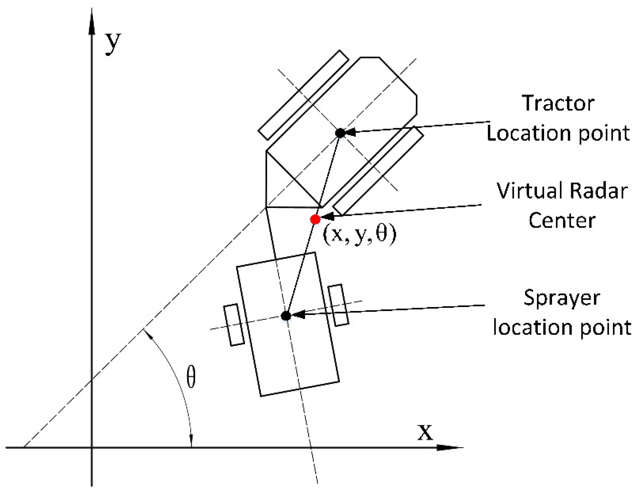
2.2. Kinematic Model of the Traction Spraying Robot

The tractor of the traction spraying robot included an electromagnetic hydraulic valve group, hydraulic cylinder and clutch. The onboard electronic control unit (ECU) outputted on-off signals by controlling the relay unit to adjust the state of the solenoid valve. Taking the forward motion state as an example, when the left track braked, the right track rotated, and the vehicle turned left. When the right track braked, the left track rotated, the vehicle turned right, and the turning radius was a fixed value. When the left and right tracks rotated at the same time, the vehicle moved forward. When the left and right tracks braked simultaneously, the vehicle stopped.

To simplify the kinematic analysis process, it was assumed that: (1) without considering the deformation, the tractor, the spraying trailer, and their connecting mechanism were rigid bodies, (2) the centroid of the tractor and spraying trailer coincided with the geometric center, (3) we could ignore the track section slip, and (4) the steering angular velocity and resistance coefficient of the crawler tractor remained unchanged during rotation [18].

The kinematic model of the traction spraying robot is shown in Figure 3. $(x_i,y_i,{\theta }_i)$ is defined as the positional information of each vehicle i = (0, 1), where $P_i(x_i,y_i)$ denotes the vehicle position coordinates, and ${\theta }_i$ denotes the heading of the vehicle (where I = 0 for the tracked tractor and i = 1 for the spraying trailer). L₀ denotes the distance from the tractor center of the mass coordinates to the hook-up point, L₁ denotes the distance from the spraying trailer center of the mass coordinates to the hook-up point, $v_0$ and $v_1$ denote, respectively, the instantaneous linear velocity of the center of mass of the tractor and the spraying trailer, and B is the tractor gauge width.

The instantaneous linear and angular velocities of the track speed and center of mass on the left and right sides of the tractor are related as in Equations (1) and (2).

$$v_0=\frac{v_L+v_R}{2},$$

(1)

$$\omega =\frac{v_R-v_L}{B},$$

(2)

Based on the kinematic principles $\dot{x}=v\cos \left(\theta \right)$ and $\dot{\theta }=\omega$, Equations (1) and (2) are brought into it to yield the kinematic equation of the tracked tractor, as shown in Equation (3).

$$\left(\begin{array}{c}{\dot{x}}_0\\ {\dot{y}}_0\\ {\dot{\theta }}_0\end{array}\right)=\left(\begin{array}{cc}\frac{\cos \left({\theta }_0\right)}{2}& \frac{\cos \left({\theta }_0\right)}{2}\\ \frac{\sin \left({\theta }_0\right)}{2}& \frac{\sin \left({\theta }_0\right)}{2}\\ \frac{1}{B}& -\frac{1}{B}\end{array}\right)\left(\begin{array}{c}{v}_R\\ v_L\end{array}\right),$$

(3)

According to the kinematic principle, the expression for the position information of the spraying trailer is shown in Equation (4).

$$\{\begin{array}{c}{\dot{x}}_1=v_1\cos \left({\theta }_1\right)\\ {\dot{y}}_1=v_1\sin \left({\theta }_1\right)\end{array},$$

(4)

The relationship between the tractor position and the spraying trailer position can be derived from the tractor unit structure in Figure 3, as shown in Equation (5).

$$\{\begin{array}{c}{x}_1=x_0-\left(L_0\cos {\theta }_0+L_1\cos {\theta }_1\right)\\ y_1=y_0-\left(L_0\sin {\theta }_0+L_1\sin {\theta }_1\right)\end{array},$$

(5)

Deriving both sides of Equation (5) and substituting into Equation (1), Equation (6) is obtained as follows.

$$\{\begin{array}{c}{v}_1\cos \left({\theta }_1\right)=v_0\cos \left({\theta }_0\right)+L_0{\dot{\theta }}_0\sin \left({\theta }_0\right)+L_1{\dot{\theta }}_1\sin \left({\theta }_1\right)\\ v_1\sin \left({\theta }_1\right)=v_0\sin \left({\theta }_0\right)-L_0{\dot{\theta }}_0\cos \left({\theta }_0\right)-L_1{\dot{\theta }}_1\cos \left({\theta }_1\right)\end{array},$$

(6)

Multiplying the first formula of Equation (6) by $\sin ({\theta }_1)$ at both ends and the second formula by $\cos ({\theta }_1)$ at both ends, then subtracting the second formula from the first, gives Equation (7).

$$v_0\left(\cos \left({\theta }_0\right)\sin \left({\theta }_1\right)-\sin \left({\theta }_0\right)\cos \left({\theta }_1\right)\right)+L_0{\dot{\theta }}_0\left(\sin \left({\theta }_0\right)\sin \left({\theta }_1\right)+\cos \left({\theta }_0\right)\cos \left({\theta }_1\right)\right)+L_1{\dot{\theta }}_1=0$$

(7)

Simplifying Equation (7) yields Equation (8):

$${\dot{\theta }}_1=\frac{1}{L_1}\left(v_0\sin \left({\theta }_0-{\theta }_1\right)-L_0{\dot{\theta }}_0\cos \left({\theta }_0-{\theta }_1\right)\right),$$

(8)

Similarly, multiplying the first formula of Equation (6) by $\cos ({\theta }_1)$ at both ends and the second formula by $\sin ({\theta }_1)$ at both ends, the two formulas are added together and simplified to give Equation (9):

$$v_1=v_0\cos \left({\theta }_0-{\theta }_1\right)+L_0{\dot{\theta }}_0\sin \left({\theta }_0-{\theta }_1\right),$$

(9)

The tractor used in this study was a single-sided brake steering, which could only control the driving state of the tracks on the left and right sides. Based on the relationship between the instantaneous linear velocity of the center of mass of the tractor and the travelling speed of the left and right side tracks (Equation (1)), the instantaneous linear velocity of the center of mass $v_0$ in Equations (8) and (9) is replaced, and the kinematic model of the tracked tractor (Equation (3)) is combined to obtain the kinematic model of the orchard traction spraying robot, as shown in Equation (10).

$$\left(\begin{array}{c}{\dot{x}}_0\\ {\dot{y}}_0\\ {\dot{\theta }}_0\\ {\dot{x}}_1\\ {\dot{y}}_1\\ {\dot{\theta }}_1\end{array}\right)=\left(\begin{array}{cc}\frac{\cos \left({\theta }_0\right)}{2}& \frac{\cos \left({\theta }_0\right)}{2}\\ \frac{\sin \left({\theta }_0\right)}{2}& \frac{\sin \left({\theta }_0\right)}{2}\\ \frac{1}{B}& -\frac{1}{B}\\ \left(\frac{\cos \left({\theta }_0-{\theta }_1\right)}{2}+\frac{L_0\sin \left({\theta }_0-{\theta }_1\right)}{B}\right)\cos \left({\theta }_1\right)& \left(\frac{\cos \left({\theta }_0-{\theta }_1\right)}{2}-\frac{L_0\sin \left({\theta }_0-{\theta }_1\right)}{B}\right)\cos \left({\theta }_1\right)\\ \left(\frac{\cos \left({\theta }_0-{\theta }_1\right)}{2}+\frac{L_0\sin \left({\theta }_0-{\theta }_1\right)}{B}\right)\sin \left({\theta }_1\right)& \left(\frac{\cos \left({\theta }_0-{\theta }_1\right)}{2}-\frac{L_0\sin \left({\theta }_0-{\theta }_1\right)}{B}\right)\sin \left({\theta }_1\right)\\ \frac{\sin \left({\theta }_0-{\theta }_1\right)}{2L_1}-\frac{L_0\cos \left({\theta }_0-{\theta }_1\right)}{B{L}_1}& \frac{\sin \left({\theta }_0-{\theta }_1\right)}{2L_1}+\frac{L_0\cos \left({\theta }_0-{\theta }_1\right)}{B{L}_1}\end{array}\right)\left(\begin{array}{c}{v}_R\\ v_L\end{array}\right),$$

(10)

Analysis of the kinematic model of the traction spraying robot shows that the relationship between the spraying trailer and the change in tractor heading is shown in Equation (11):

$$\frac{{\dot{\theta }}_1}{{\dot{\theta }}_0}=\frac{\sqrt{B^2+L_0{}^2}}{L_1}\sin \left({\theta }_0-{\theta }_1-\arctan \frac{L_0}{B}\right),$$

(11)

When ${\theta }_0={\theta }_1$, i.e., the spraying trailer heading angle is equal to the tractor heading angle, there is ${\dot{\theta }}_1/{\dot{\theta }}_0=-L_0/L_1$, i.e., at this time, the heading change of the spraying trailer is opposite to that of the tractor, and the size is inversely proportional to the distance from the respective steering center to the hanging point.

2.3. Double-DQN Model Development

2.3.1. Double-DQN Network Architecture

We used the Double-DQN network structure, in which each action of the traction spraying robot had a separate output unit, i.e., turn left, turn right, and go straight. The state of the traction spraying robot was taken as the input of the neural network. The main advantage of this architecture is the ability to calculate the Q value of all actions in a given state with only one forward pass in the network [19].

In this study, the scanning result of a virtual radar on a virtual boundary was defined as a virtual radar map. The scanning of the virtual radar on the virtual path boundary could reflect the path deviation and path change of the tractor [9]. As shown in Figure 4, the starting point of the straight part of the reference path is $S(x_s,y_s)$, and the endpoint is $E(x_e,y_e)$. The width of the virtual path is d. The green graph in the figure shows the image detected by the virtual radar, which consists of four edges, of which the straight line segment is the detected virtual path boundary, and the circular arc segment is the maximum detection boundary of the radar. As shown in Figure 5, the virtual radar map positioning point is the midpoint of the connection between the tractor positioning point and the spraying trailer positioning point, for which $\theta$ is the course of the tractor. Using the virtual radar map as input to the Double-DQN network, the network structure and composition of the input and output layers are shown in Figure 6. To solve the path-tracking control problem, we made use of the optimal Q-value (action value) for each action. The Q-values for a series of given actions (the desired action in this study) were the output of the network, and a given state s was used as the network input. Each Q-value represented the expected future tracking performance of the corresponding steering action. Therefore, the action with the largest Q-value was selected.

The network architecture proposed in this study for training and control has six layers, including an input layer, four fully connected hidden layers, and an output layer, as shown in Figure 7. Based on Python 3.5, this study constructed a neural network model based on Windows10 using Google’s open-source deep learning framework, TensorFlow2.0 (GPU). Specifically, the network was built using the Sequential model in Keras. There are 360 neurons in the input layer and 3 neurons in the output layer, corresponding to 3 predefined actions. The activation function is the sigmoid function [6]. Each hidden fully connected layer has 100 neurons, and the activation function is a rectification linear function. In this study, we determined the network structure by balancing the generalization ability and computational cost of the model. A simple network has fast calculation speed but poor generalization ability. Complex networks have strong generalization ability but need a long training time. When determining the model structure, we used the upper limit and rising speed of reward scores in network training as evaluation criteria. The values of the network hyperparameters are shown in

Table 2. List of hyperparameters and their values.

Hyperparameter	Value
Minibatch size	16
Replay memory size	20,000
update frequency	200
Discount factor γ	0.99
Learning rate	0.0001
Initial exploration ε	0.9

.

2.3.2. Double-DQN Training Algorithm

Double-DQN is an improved algorithm of the classical deep reinforcement learning algorithm DQN (Deep Q Network). Double-DQN solves the overestimation problem in DQN to a certain extent and improves the stability of the algorithm [20]. The flow of the Double-DQN agent training algorithm is shown in Figure 8.

The agent (traction spraying robot) was trained for autonomous learning by first initializing the memory playback unit and the network parameters $\theta$ and ${\theta }^{-}$ of the current value network and the target value network. Then, $s$ was initialized as the first state of the current state sequence; we subsequently selected action $a$ and executed it using the $\epsilon \text{-}\mathrm{greedy}$ algorithm to obtain the next state $s^{\prime }$, immediately return r, and store $(s,a,r,s^{\prime })$ in the memory playback unit. Each time a certain number of parameters were adjusted, a certain number of samples were randomly collected in the memory playback unit for gradient descent to solve the current value network parameters. Because the weight of the network is updated by gradient backpropagation, if the input data are sequential, it will lead to overestimation. Collecting a certain number of samples can improve training efficiency by disrupting the batch of input data. At regular intervals, the current value network parameters were assigned to the target value network so that the agent training was completed iteratively [21].

A reward is an incentive mechanism designed by people using prior knowledge to encourage reinforcement learning algorithms to learn in the direction of people’s expectations. For path-following autonomous learning, we designed a sparse reward [22]. The rules for the incentive mechanism (12) were established as shown below. If R is a reward for the agent’s action in the current state, when the agent made the correct action for the state, a reward of 1 was given; otherwise, a reward of −1 was given, and when the lateral deviation between the agent and the reference path was 0, a reward of 0 was given.

The network requires a large amount of data to be trained. In order to do this, each time the simulated line tracking process was run until the agent successfully reached the endpoint, the process was stored and then used for empirical replay [23]. $\mathsf{\Delta }{d}_1$ denotes the lateral deviation value of the intelligent body in state $s^{\prime }$, $\mathsf{\Delta }{\theta }_1$ denotes the heading deviation value of the agent in state $s^{\prime }$, and $\mathsf{\Delta }{\theta }_0$ denotes the heading deviation value of the agent in state $s$. The initial state $s$ and action $a$ are randomly established in the set range. $\mathsf{\Delta }{d}_1$ is in the range [−700, 700], and $\mathsf{\Delta }{\theta }_1$ and $\mathsf{\Delta }{\theta }_0$ are in the range (−π/2, π/2). When the lateral deviation and heading deviation took a positive value, it meant that it was on the left side of the planned path and vice versa for the right side. The value of action $a$ is [0, 1, 2] (0 for straight, 1 for left, 2 for right). When the agent was outside the set range, the agent reverted to the starting point.

$$R=\{\begin{array}{c}+1\\ 0\\ -1\end{array}\begin{array}{c}\mathsf{\Delta }{d}_1\ne 0,\mathsf{\Delta }{\theta }_1\in (-\pi /2,\pi /2), \mathrm{Predefined} \mathrm{action} \mathrm{driving}\\ \mathsf{\Delta }{d}_1=0,\mathsf{\Delta }{\theta }_1\in (-\pi /2,\pi /2)\\ \mathsf{\Delta }{d}_1\ne 0,\mathsf{\Delta }{\theta }_1\in (-\pi /2,\pi /2), \mathrm{Non}\text{-}\mathrm{predefined} \mathrm{action} \mathrm{driving}\end{array},$$

(12)

According to the rules of the reward mechanism, the reward and punishment values of specific actions in different states of the agent could be obtained, as shown in

Table 3. Reward and punishment values for the left side of the planning path.

$\mathsf{\Delta }{\mathit{d}}_1$	$\mathsf{\Delta }{\mathit{\theta }}_1$	$\mathit{R}$
(0, 70]	(−90, −10]	1 (left turn)
		−1 (other actions)
	(−10, 0)	1 (straight)
		−1 (other actions)
	[0, 90)	1 (right)
		−1 (other actions)
(70, 150]	(−90, −20]	1 (left)
		−1 (other actions)
	(−20, −12)	1 (straight)
		−1 (other actions)
	[−12, 90)	1 (right)
		−1 (other actions)
(150, 700]	(−90, −30]	1 (left)
		−1 (other actions)
	(−30, −22)	1 (straight)
		−1 (other actions)
	[−22, 90)	1 (right)
		−1 (other actions)

and

Table 4. Reward and punishment values for the right side of the planning path.

$\mathsf{\Delta }{\mathit{d}}_1$	$\mathsf{\Delta }{\mathit{\theta }}_1$	$\mathit{R}$
[−70, 0)	(−90, 0]	1 (left)
		−1 (other actions)
	(0, 10)	1 (straight)
		−1 (other actions)
	[10, 90)	1 (right)
		−1 (other actions)
[−150, −70)	(−90, 12]	1 (left)
		−1 (other actions)
	(12, 20)	1 (straight)
		−1 (other actions)
	[20, 90)	1 (right)
		−1 (other actions)
[−700, −150)	(−90, 22]	1 (left)
		−1 (other actions)
	(22, 30)	1 (straight)
		−1 (other actions)
	[30, 90)	1 (right)
		−1 (other actions)

. Here, $\mathsf{\Delta }{\theta }_1>\mathsf{\Delta }{\theta }_0$ for left, $\mathsf{\Delta }{\theta }_1=\mathsf{\Delta }{\theta }_0$ for straight, and $\mathsf{\Delta }{\theta }_1<\mathsf{\Delta }{\theta }_0$ for right.

3. Simulation Test Results

3.1. Simulation Environment Creation

The simulation environment of this study was based on Python 3.5, the PyQt5 framework and Google’s open-source deep learning program framework, TensorFlow2.0 (GPU version). The running environment was a Windows 10 system; the simulation environment is shown in Figure 9. The agent model represents the traction spraying robot, the reference path fold line represents the operation path, and the solid dots represent the starting and ending points of the planned path. The reference path parameters are shown in Figure 10, with the reference path starting point being (0, 0) m and the reference path endpoint being (5.0, 8.0) m.

The relevant network parameters and training hyperparameters were set according to the previous sections. The current value network and the target value network were structurally consistent. In the simulation experiment, the storage capacity of the memory playback unit was set to 90,000, and the network parameters of the target value network were copied to the current value network parameters once for each 200-parameter adjustment so as to reduce the correlation between the two networks and improve the network training efficiency. The $\epsilon$ value of the $\epsilon \text{-}\mathrm{greedy}$ algorithm was set to 0.9 to improve the exploration ability of the intelligence, i.e., a 0.9 probability of selecting the action with the largest value of state behavior for execution; otherwise, a random action was selected for execution, and the decay factor of the $\epsilon \text{-}\mathrm{greedy}$ algorithm was set to 0.0001. The training of the agent ended when the network converged to a certain extent.

The agent started from the starting point of the reference path. In order to make the agent’s exploratory learning more comprehensive, we added random disturbance to the agent’s kinematics model, and the random disturbance deviation range was [−20, 20] mm. If the lateral deviation or heading deviation of the agent from the reference path were greater than the set threshold, the agent ended the round and returned to the origin to start the next round of training again. The agent reaching the end of the reference path was regarded as the success of this round of learning.

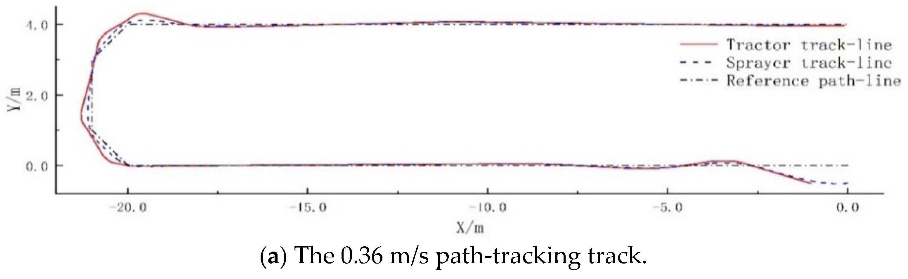
3.2. Simulation Test Results

The single-step reward results of agent training are shown in Figure 11. The abscissa represents the number of training steps, and the ordinate represents the reward value of each step. The total number of agent training steps was 23,296 steps. With the increase in training steps, the reward value tended to be stable, and the score of each round increased gradually. The scoring results of each round of agent training are shown in Figure 12. At the beginning of the training, the score was low, and the score changed greatly. As the number of rounds increased, the score became larger, and the data tended to be stable. The success rate of agent training is shown in Figure 13. The agent reached the end of the reference path in the fifth round. As the training continued, the success rate of the agent continued to increase.

The results of the training and testing of the agent showed the value and potential of this idea of autonomous learning using an agent. The advantage of reinforcement learning is that an agent without excessive a priori knowledge could learn some of the common experiences of artificial design through continuous interaction with the environment and may even discover some experiences that have not been learned by engineers [20,21].

3.3. Validation of Simulation Results

To verify the feasibility of the path-tracking algorithm proposed in the study, simulation experiments were carried out in a simulation environment. The path planned for the simulation is a ‘U’-shaped folding path, 20 m long and 4 m wide (total path length is approximately 42.83 m), with a path starting point of (0, 0) m and a path end point of (0, 4.0) m. The initial lateral deviation of the kinematic model of the traction spraying robot was 0.5 m, and the heading angle was 180°. The simulation verification was carried out at two speeds of 0.36 m/s and 0.75 m/s. During the simulation process, the communication, display and data recording of the upper control system were normal, and the simulation test results are shown in Figure 14.

When the simulation speed was 0.36 m/s, the maximum lateral deviation of the spraying trailer path tracking was 0.117 m, the average lateral deviation was 0.038 m, and the standard deviation was 0.028 m. When the simulation speed was 0.75 m/s, the maximum lateral deviation of the spraying trailer path tracking was 0.119 m, the average lateral deviation was 0.040 m, and the standard deviation was 0.029 m. The simulation results showed that the Double-DQN-based orchard traction spraying robot navigation path-tracking control algorithm was feasible in principle for navigation path-tracking control, and the spraying trailer had high path-tracking accuracy to meet practical operational needs.

4. Field Test Results

Experimental Results of Robot Path-Tracking Control Algorithm

Our team used a portable differential positioning device (Figure 15) to verify the method of calculating the position of the spraying trailer by the established kinematic model of the traction spraying robot. For the verification test, our team carried out a portable differential positioning equipment accuracy test and kinematic model to calculate the spraying trailer pose information method validation test. The test results showed that the fixed differential signal of the portable differential positioning equipment was stable and met the requirements of this study. The position of the spraying trailer calculated by the kinematic model had the same trend as the position trajectory of the spraying trailer actually recorded by the portable differential positioning device. The experimental results showed that the kinematic model established in this study could better reflect the kinematic characteristics of the orchard traction spraying robot and had higher accuracy. To a certain extent, it could replace the sensor to calculate the position of the spraying trailer in the actual operation process of the orchard traction spraying robot, saving the cost of the equipment.

The experimental field of the path-tracking control algorithm for the traction spraying robot was located in the National Persimmon Germplasm Resources Garden of Northwest A&F University (108.066° E, 34.297° N). As shown in Figure 16, the row spacing of fruit trees is 2.4 m, and the plant spacing is about 2~3 m.

The field test site is shown in Figure 17. Considering that the robot needed to follow a straight line and turn around to change rows during the orchard operation, the planned path was designed as a 20.0 × 2.4 m ‘U’-shaped folding path, and the test speed was set at 0.36 m/s and 0.75 m/s. To ensure the validity of the test data, each set of tests was repeated three times (the lateral and heading deviations in the test results are absolute values). The results of the path-tracking tests are shown in Figure 18, the statistics of the repeated tests are shown in

Table 5. Path-tracking experimental data.

v/(m/s)	Test No.	Sprayer Path-Tracking Deviation
		Maximum Lateral Deviation /(m)		Average Lateral Deviation /(m)		Standard Deviation/(m)
		Straight Line (0~20 m)	Full Range	Straight Line (0~20 m)	Full Range	Straight Line (0~20 m)	Full Range
0.36	r361	0.128	0.233	0.043	0.070	0.026	0.051
	r362	0.120	0.225	0.041	0.069	0.025	0.049
	r363	0.134	0.240	0.045	0.073	0.028	0.054
	$\overline{\mathrm{r}36}$	0.127	0.233	0.043	0.071	0.026	0.051
	l361	0.126	0.536	0.051	0.084	0.021	0.059
	l362	0.146	0.558	0.061	0.080	0.023	0.069
	l363	0.113	0.509	0.056	0.066	0.026	0.063
	$\overline{\mathrm{l}36}$	0.128	0.534	0.056	0.077	0.023	0.064
0.75	r751	0.145	0.263	0.055	0.076	0.033	0.056
	r752	0.155	0.275	0.057	0.079	0.034	0.058
	r753	0.140	0.259	0.054	0.074	0.032	0.056
	$\overline{\mathrm{r}75}$	0.147	0.266	0.055	0.076	0.033	0.057
	l751	0.149	0.536	0.057	0.081	0.030	0.062
	l752	0.178	0.554	0.054	0.081	0.034	0.066
	l753	0.207	0.558	0.061	0.078	0.034	0.059
	$\overline{\mathrm{l}75}$	0.178	0.549	0.057	0.080	0.033	0.062

Note: Test number r361 stands for the Double-DQN algorithm path-tracking test group 1 at 0.36 m/s speed, l361 stands for the virtual radar control algorithm path-tracking test group 1 at 0.36 m/s speed, $\overline{\mathrm{r}36}$ stands for the average of the Double-DQN algorithm control at 0.36 m/s speed for 3 sets of test results, and $\overline{\mathrm{l}36}$ stands for the average of the virtual radar model control at 0.36 m/s speed.

, and the three-dimensional diagrams of the path-tracking errors for the two control methods are shown in Figure 19.

From Figure 18 and Figure 19, it can be seen that under the same speed, the path-tracking algorithm based on Double-DQN had a smaller overall lateral deviation in the whole path of the spraying trailer compared with the path-tracking algorithm based on the virtual radar model [9]. The spraying trailer had better path-tracking accuracy and driving stability in the turning process and the straight-line driving part after lane changing.

The results of comparing the tracking accuracy of the straight path portion (‘U’-shaped fold path 0~20 m) of the spraying trailer for the two control algorithms are shown in

Table 6. Comparison of straight-line path-tracking accuracy.

v/(m/s)	Test No.	Maximum Lateral Deviation /(m)	Average Lateral Deviation /(m)	Standard Deviation /(m)
0.36	$\overline{\mathrm{r}36}$	0.127	0.043	0.026
	$\overline{\mathrm{l}36}$	0.128	0.056	0.023
		−0.001 (0.78%)	−0.013 (23.21%)	0.003 (13.04%)
0.75	$\overline{\mathrm{r}75}$	0.147	0.055	0.033
	$\overline{\mathrm{l}75}$	0.178	0.057	0.033
		−0.031 (17.41%)	−0.002 (3.51%)	0 (0%)

. At the speed of 0.36 m/s, the virtual radar model algorithm was superior to the Double-DQN algorithm in terms of the driving stability (standard deviation) of the spraying trailer. However, the algorithm proposed in this study was superior to the virtual radar model algorithm in terms of the average lateral deviation and maximum lateral deviation. The average lateral deviation and maximum lateral deviation were reduced by 23.21% and 0.78%, respectively. At the speed of 0.75 m/s, the driving stability (standard deviation) of the spraying trailer proposed in this study was consistent, but it was superior to the virtual radar model algorithm in terms of average lateral deviation and maximum lateral deviation. The maximum lateral deviation and average lateral deviation were reduced by 17.41% and 3.51%, respectively.

Comparing the ‘U’-shaped path-tracking accuracy of the spraying trailer under the two navigation path-tracking control algorithms, the results are shown in

Table 7. Comparison of ‘U’-shaped path-tracking accuracy.

v/(m/s)	Test No.	Maximum Lateral Deviation /(m)	Average Lateral Deviation /(m)	Standard Deviation /(m)
0.36	$\overline{\mathrm{r}36}$	0.233	0.071	0.051
	$\overline{\mathrm{l}36}$	0.534	0.077	0.064
		−0.301 (56.37%)	−0.006 (7.8%)	0.013 (20.31%)
0.75	$\overline{\mathrm{r}75}$	0.266	0.076	0.057
	$\overline{\mathrm{l}75}$	0.549	0.080	0.062
		−0.283 (51.54%)	−0.004 (5.0%)	−0.005 (8.1%)

. All path-tracking indexes of the proposed algorithm were better than those of the virtual radar model algorithm. The maximum lateral deviation was reduced by 56.37%, the average lateral deviation was reduced by 7.8%, and the standard deviation was reduced by 20.31%. This showed that the overall path-tracking performance of the new algorithm in the ‘U’-shaped path was significantly better than that of the tracking algorithm based on the virtual radar model.

Comparing the tracking accuracy of the ‘U’-shaped path and the straight path of the spraying trailer under the two algorithms, the results are shown in

Table 8. Comparison of ‘U’-shaped and straight line path-tracking accuracy.

v/(m/s)	Path Shape	Test No.	Maximum Lateral Deviation /(m)	Average Lateral Deviation /(m)	Standard Deviation /(m)
0.36	Straight	$\overline{\mathrm{r}36}$	0.127	0.043	0.026
	‘U’-shaped	$\overline{\mathrm{r}36}$	0.233	0.071	0.051
			0.106 (83.46%)	0.028 (65.12%)	0.025 (96.15%)
	Straight	$\overline{\mathrm{l}36}$	0.128	0.056	0.023
	‘U’-shaped	$\overline{\mathrm{l}36}$	0.534	0.077	0.064
			0.406 (317.19%)	0.021 (37.5%)	0.041 (178.26%)
0.75	Straight	$\overline{\mathrm{r}75}$	0.147	0.055	0.033
	‘U’-shaped	$\overline{\mathrm{r}75}$	0.266	0.076	0.057
			0.119 (80.95%)	0.021 (38.18%)	0.024 (72.72%)
	Straight	$\overline{\mathrm{l}75}$	0.178	0.057	0.033
	‘U’-shaped	$\overline{\mathrm{l}75}$	0.549	0.080	0.062
			0.371 (208.43%)	0.023 (40.35%)	0.029 (87.88%)

. The tracking accuracy indexes of the ‘U’-shaped path and straight path based on the virtual radar model were quite different, especially the maximum lateral deviation. When the speed was 0.36 m/s and 0.75 m/s, the maximum lateral deviation of the ‘U’-shaped path based on the virtual radar model was 317.19% and 208.43% higher than the maximum lateral deviation of the straight path, while the relevant indicators of the proposed algorithm were relatively similar. When the speed was 0.36 m/s and 0.75 m/s, the maximum lateral deviation of the ‘U’-shaped path was 83.46% and 80.95% higher than the maximum lateral deviation of the straight path. It showed that the deviation control ability of the new algorithm was better than that of the virtual radar model control and had better steering path adaptability.

The statistical results of the path-tracking data of the spraying trailer and tractor were analyzed, as shown in

Table 9. Comparison of spraying trailer and tractor path tracking.

v/(m/s)	Model	Test No.	Maximum Lateral Deviation /(m)	Average Lateral Deviation /(m)	Standard Deviation /(m)
0.36	Tractor	$\overline{\mathrm{r}36}$	0.382	0.087	0.075
	Trailer	$\overline{\mathrm{r}36}$	0.233	0.071	0.051
			−0.149 (39.0%)	−0.016 (18.39%)	−0.024 (32%)
	Tractor	$\overline{\mathrm{l}36}$	0.150	0.031	0.025
	Trailer	$\overline{\mathrm{l}36}$	0.534	0.077	0.064
			0.384 (256.0%)	0.046 (148.39%)	0.039 (156.0%)
0.75	Tractor	$\overline{\mathrm{r}75}$	0.448	0.110	0.095
	Trailer	$\overline{\mathrm{r}75}$	0.266	0.076	0.057
			−0.222 (45.5%)	−0.034 (30.9%)	−0.038 (40%)
	Tractor	$\overline{\mathrm{l}75}$	0.191	0.051	0.036
	Trailer	$\overline{\mathrm{l}75}$	0.549	0.080	0.062
			0.358 (187.43%)	0.029 (56.86%)	0.026 (72.22%)

. The path-tracking accuracy indexes of the spraying trailer and tractor based on the virtual radar model were quite different, especially the maximum lateral deviation. When the speed was 0.36 m/s and 0.75 m/s, the maximum lateral deviation of the spraying trailer path tracking was 256.0% and 187.43% higher than that of the tractor path tracking. The relevant indicators of the proposed algorithm were relatively similar. When the speed was 0.36 m/s and 0.75 m/s, the maximum lateral deviation of the spraying trailer path tracking was 39.0% and 45.5% lower than the maximum lateral deviation of the tractor path tracking. It showed that the new algorithm had better control ability than the virtual radar model control for spraying trailer path tracking.

5. Discussion

The automatic navigation of the traction spraying robot should not only focus on the position change of the tractor during its navigation and driving but also on whether the spraying trailer can effectively track the planned orchard operation path. In order to improve the path-tracking control accuracy and driving stability of the orchard traction spraying robot, this study proposed a navigation path-tracking control algorithm based on the Double Deep Q-Network (Double DQN). The algorithm was tested in both simulations and on a field to follow a typical ‘U’-shaped path. The simulation results showed that the proposed algorithm was able to achieve accurate path-tracking control of the spraying trailer. The field tests showed that when the vehicle speed was 0.36 m/s and 0.75 m/s, the maximum lateral deviation of the algorithm was 0.233 m and 0.266 m, the average lateral deviation was 0.071 m and 0.076 m, and the standard deviation was 0.051 m and 0.057 m, respectively. Compared with the algorithm based on the virtual radar model [6], the maximum lateral deviation was reduced by 56.37% and 51.54%, the average lateral deviation was reduced by 7.8% and 5.0%, and the standard deviation was reduced by 20.31% and 8.1%, respectively.

Although the trajectory of the spraying trailer is controlled, compared with the simulation test, the indicators of the path tracking of the spraying trailer in the field test were quite different. The test comparison data are shown in

Table 10. Comparison of simulation and field experiment path-tracking accuracy.

v/(m/s)	Test Type	Maximum Lateral Deviation /(m)	Average Lateral Deviation /(m)	Standard Deviation /(m)
0.36	Simulation	0.117	0.038	0.028
	Field	0.233	0.071	0.051
		0.116 (99.14%)	0.033 (86.84%)	0.023 (82.14%)
0.75	Simulation	0.119	0.040	0.029
	Field	0.266	0.076	0.057
		0.147 (123.53%)	0.036 (90%)	0.028 (96.55%)

. When the vehicle speed was 0.36 m/s and 0.75 m/s, the maximum lateral deviation of the spraying trailer path tracking in the field experiment increased by 99.147% and 123.53%, the average lateral deviation increased by 86.84% and 90%, and the standard deviation increased by 82.14% and 96.55%, respectively. The main possible reasons for this are as follows: (1) in order to save costs, we used a set of positioning systems to obtain the position information of the tractor and estimate the position information of the spraying trailer through the kinematic model. The angle difference between the heading angle of the tractor and the spraying trailer was not taken into account, which may lead to deviation errors. (2) The tractor control device was simple, and the tractor had a reaction time from receiving the signal to performing the corresponding action, which may lead to deviation errors. (3) With the increase in the speed of the traction spraying robot, the navigation path-tracking accuracy of the spraying trailer was reduced. Due to the simple control device of the tractor in this study, the influence of different speeds on the control accuracy was not considered, which may lead to deviation errors. (4) When the robot was working in the orchard, the GNSS signal drifted briefly, which may lead to deviation errors.

Future work will focus on: (1) in the stage of establishing the kinematics model of the traction spraying robot, the relevant parameters at the connection of the spraying trailer will be added, such as the angle difference between the yaw angle of the tractor and the spraying trailer, so as to include this interaction in the design stage, which may achieve a better control effect; (2) in the aspect of optimizing the control algorithm, we suggest studying the influence of virtual radar model parameters, the neural network structure and parameter changes on navigation effect; (3) we propose studying the influence of speed changes on navigation effectso that the control model can adapt to the effect of speed variation; and (4) we recommend using 3D radar sensors to sense the environment, as through multi-sensor data fusion, we can deal with the interference caused by trunk occlusion.

6. Conclusions

In this paper, in order to improve the precision and driving stability of a spraying trailer tracking a predefined trajectory in a traction spraying robot, this study proposed a navigation path-tracking control algorithm based on the Double-DQN method. The Double-DQN method is an optimal decision-making method based on state space. This method is different from the supervised learning method. It does not need to be trained according to the sample. The control standard (using the reward function) learned in the simulation environment can optimize the tracking performance. It does not depend on complex mathematical models and is easy to expand. In order to reduce the cost of use and facilitate practical application, we used a set of positioning systems to obtain the pose information of the tractor, combined the kinematics model of the traction spraying robot to calculate the pose information of the spraying trailer in real-time, and analyzed the path-tracking effect of the spraying trailer.

The algorithm was tested in both simulations and on a field to follow a typical ‘U’-shaped path. The simulation results showed that when the speed was 0.36 m/s, the maximum lateral deviation of the spraying trailer path tracking was 0.117 m; when the speed was 0.75 m/s, the maximum lateral deviation of the spraying trailer path tracking was 0.119 m. This showed that the proposed algorithm could realize the navigation path-tracking control of the spraying trailer in principle and had a high control accuracy, which could meet the needs of the orchard’s autonomous spraying operation. The field test results showed that when the vehicle speed was 0.36 m/s and 0.75 m/s, compared with the control algorithm of the virtual radar model, the maximum lateral deviation of the spraying trailer was reduced by 56.37% and 51.54%, respectively, the average lateral deviation was reduced by 7.8% and 5.0%, respectively, and the standard deviation was reduced by 20.31% and 8.1%, respectively. It showed that the overall performance of the algorithm was better than the control algorithm based on the virtual radar model, which effectively improved the tracking accuracy of the navigation path of the spraying trailer and the stability of the automatic operation and had better adaptability to the typical operation path of the orchard.

References

1. Zhao, Y.; Xiao, H.; Mei, S.; Song, Z.; Ding, W.; Jin, Y.; Han, Y.; Xia, X.; Yang, G. Current status and development strategies of mechanized orchard production in China. J. China Agric. Univ. 2017, 22, 116–127. [Google Scholar]
2. Zheng, Y.J.; Jiang, W.; Chen, B.T.; Lu, H.; Wan, C.; Kang, F. Advances in mechanization technology and equipment for orchards in hilly mountainous areas. J. Agric. Mach. 2020, 51, 1–20. [Google Scholar]
3. He, X. Research status and development suggestions on precision application technology and equipment in China. Smart Agric. 2020, 2, 133–146. [Google Scholar]
4. Lu, C.; Nie, P.; Wang, L.; Wang, J.; Tao, J. Overview of orchard mechanization development in China Deciduous Fruit Trees. J. Deciduous Fruits 2018, 50, 30–31. [Google Scholar]
5. Jing, Y.; Liu, G.; Jin, Z. Navigation sideslip estimation and adaptive control method for farm grader. J. Agric. Mach. 2020, 51, 26–33. [Google Scholar]
6. Liu, Z.J.; Wang, S.L.; Ren, Z.G.; Mao, W.J.; Yang, F.Z. A virtual radar model-based navigation path tracking control algorithm for crawler tractors. J. Agric. Mach. 2021, 52, 376–385. [Google Scholar]
7. Wang, S.; Song, J.; Qi, P.; Yuan, C.; Wu, H.; Zhang, L.; Liu, W.; Liu, Y.; He, X. Design and development of orchard autonomous navigation spray system. Front. Plant Sci. 2022, 13, 960686. [Google Scholar] [CrossRef] [PubMed]
8. Murillo, M.; Sánchez, G.; Deniz, N.; Genzelis, L.; Giovanini, L. Improving path-tracking performance of an articulated tractor-trailer system using a non-linear kinematic model. Comput. Electron. Agric. 2022, 196, 106826. [Google Scholar] [CrossRef]
9. Backman, J.; Oksanen, T.; Visala, A. Navigation system for agricultural machines: Nonlinear Model Predictive path tracking. Comput. Electron. Agric. 2012, 82, 32–43. [Google Scholar] [CrossRef]
10. Rawlings, J.B.; Risbeck, M.J. Model predictive control with discrete actuators: Theory and application. Automatica 2017, 78, 258–265. [Google Scholar] [CrossRef]
11. Kayacan, E.; Kayacan, E.; Ramon, H.; Saeys, W. Distributed nonlinear model predictive control of an autonomous tractor–trailer system. Mechatronics 2014, 24, 926–933. [Google Scholar] [CrossRef]
12. Yue, M.; Wu, X.; Guo, L.; Gao, J. Quintic Polynomial-based Obstacle Avoidance Trajectory Planning and Tracking Control Framework for Tractor-trailer System. Int. J. Control Autom. Syst. 2019, 17, 2634–2646. [Google Scholar] [CrossRef]
13. Kayacan, E.; Ramon, H.; Saeys, W. Robust Trajectory Tracking Error Model-Based Predictive Control for Unmanned Ground Vehicles. IEEE/ASME Trans. Mechatron. 2015, 21, 806–814. [Google Scholar] [CrossRef]
14. Tang, L.; Yan, F.; Zou, B.; Wang, K.; Lv, C. An Improved Kinematic Model Predictive Control for High-Speed Path Tracking of Autonomous Vehicles. IEEE Access 2020, 8, 51400–51413. [Google Scholar] [CrossRef]
15. Mondal, K.; Rodriguez, A.A.; Manne, S.S.; Das, N.; Wallace, B. Comparison of Kinematic and Dynamic Model Based Linear Model Predictive Control of Non-Holonomic Robot for Trajectory Tracking: Critical Trade-offs Addressed. In Proceedings of the Control and Optimization of Renewable Energy Systems/860: Mechatronics and Control, Anaheim, CA, USA, 6–7 December 2019. [Google Scholar]
16. Kong, J.; Pfeiffer, M.; Schildbach, G.; Borrelli, F. Kinematic and dynamic vehicle models for autonomous driving control design. In Proceedings of the 2015 IEEE Intelligent Vehicles Symposium (IV), Seoul, Korea, 28 June–1 July 2015; pp. 1094–1099. [Google Scholar]
17. Werner, R.; Mueller, S.; Kormann, G. Path Tracking Control of Tractors and Steerable Towed Implements Based On Kinematic and Dynamic Modeling. In Proceedings of the 11th International Conference on Precision Agriculture, Indianapolis, IN, USA, 16 July 2012; pp. 15–18. [Google Scholar]
18. Ding, Y.; He, Z.; Xia, Z.; Peng, J.; Wu, T. Design of a navigation-immune PID controller for a small tracked rape planter. J. Agric. Eng. 2019, 35, 12–20. [Google Scholar]
19. Mnih, V.; Kavukcuoglu, K.; Silver, D.; Rusu, A.A.; Veness, J.; Bellemare, M.G.; Graves, A.; Riedmiller, M.; Fidjeland, A.K.; Ostrovski, G.; et al. Human-level control through deep reinforcement learning. Nature 2015, 518, 529–533. [Google Scholar] [CrossRef] [PubMed]
20. Huang, X.; Liu, J.R.; Luo, I. Parameter design of launch vehicle attitude controller based on DDQN Space Control. Aerosp. Control 2020, 38, 3–8. [Google Scholar] [CrossRef]
21. Guo, S.; Zhang, X.; Du, Y.; Zheng, Y.; Cao, Z. Path Planning of Coastal Ships Based on Optimized DQN Reward Function. J. Mar. Sci. Eng. 2021, 9, 210. [Google Scholar] [CrossRef]
22. Yang, Q.; Wang, S.; Sang, J.; Wang, C.; Huang, G.; Wu, C.; Song, S. Intelligent ship path planning and obstacle avoidance methods in complex open water. Comput. Integr. Manuf. Syst. 2022, 28, 2030–2040. [Google Scholar] [CrossRef]
23. Shan, Y.; Zheng, B.; Chen, L.; Chen, L.; Chen, D. A Reinforcement Learning-Based Adaptive Path Tracking Approach for Autonomous Driving. IEEE Trans. Veh. Technol. 2020, 69, 10581–10595. [Google Scholar] [CrossRef]
Figure 1. Orchard traction spraying robot.
Agronomy 12 02803 g001
Figure 2. Structure of the navigation control system of the orchard traction spraying robot.
Agronomy 12 02803 g002
Figure 3. Kinematic model of the orchard traction spraying robot.
Agronomy 12 02803 g003
Figure 4. Schematic illustration of the virtual radar map generation.
Agronomy 12 02803 g004
Figure 5. Schematic illustration of the main parameters of the virtual radar diagram of the orchard traction spraying robot.
Agronomy 12 02803 g005
Figure 6. Overview of the network structure and the formation of its input and output layers.
Agronomy 12 02803 g006
Figure 7. Schematic illustration of the Double-DQN network.
Agronomy 12 02803 g007
Figure 8. Agent training algorithm flowchart.
Agronomy 12 02803 g008
Figure 9. The agent simulation environment.
Agronomy 12 02803 g009
Figure 10. Schematic illustration of reference path.
Agronomy 12 02803 g010
Figure 11. Agent training single-step rewards.
Agronomy 12 02803 g011
Figure 12. The agent trains to score points per turn.
Agronomy 12 02803 g012
Figure 13. Agent training success rate.
Agronomy 12 02803 g013
Figure 14. Simulation experimental results.
Agronomy 12 02803 g014aAgronomy 12 02803 g014b
Figure 15. Portable differential positioning devices.
Agronomy 12 02803 g015
Figure 16. Orchard traction spraying robot test site.
Agronomy 12 02803 g016
Figure 17. Navigation path-tracking real vehicle experiment.
Agronomy 12 02803 g017
Figure 18. Results of the real vehicle experiment.
Agronomy 12 02803 g018
Figure 19. (a,b) The 3D maps of 0.36 m/s and 0.75 m/s path-tracking error for the Double-DQN method; (c,d) 3D maps of 0.36 m/s and 0.75 m/s path-tracking error for the virtual radar method.
Agronomy 12 02803 g019