
Impact of Conservation Agriculture on Soil Erosion in the Annual Cropland of the Apulia Region (Southern Italy) Based on the RUSLE-GIS-GEE Framework

 ,
,  , and
, and 
Abstract
:1. Introduction
2. Materials and Methods
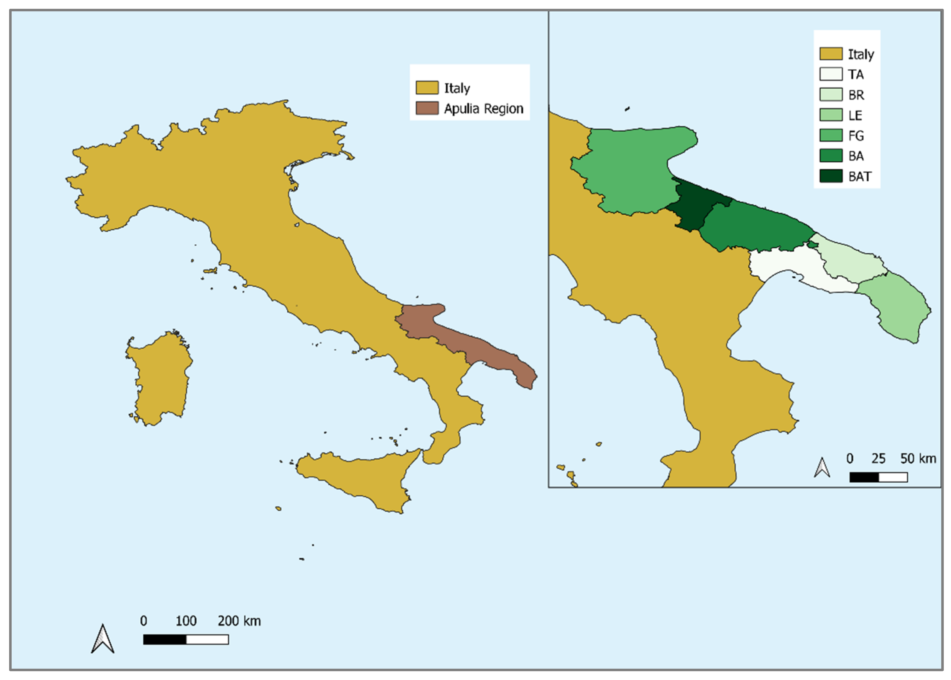
2.1. Study Area
2.2. Soil Loss Modeling: RUSLE Factors
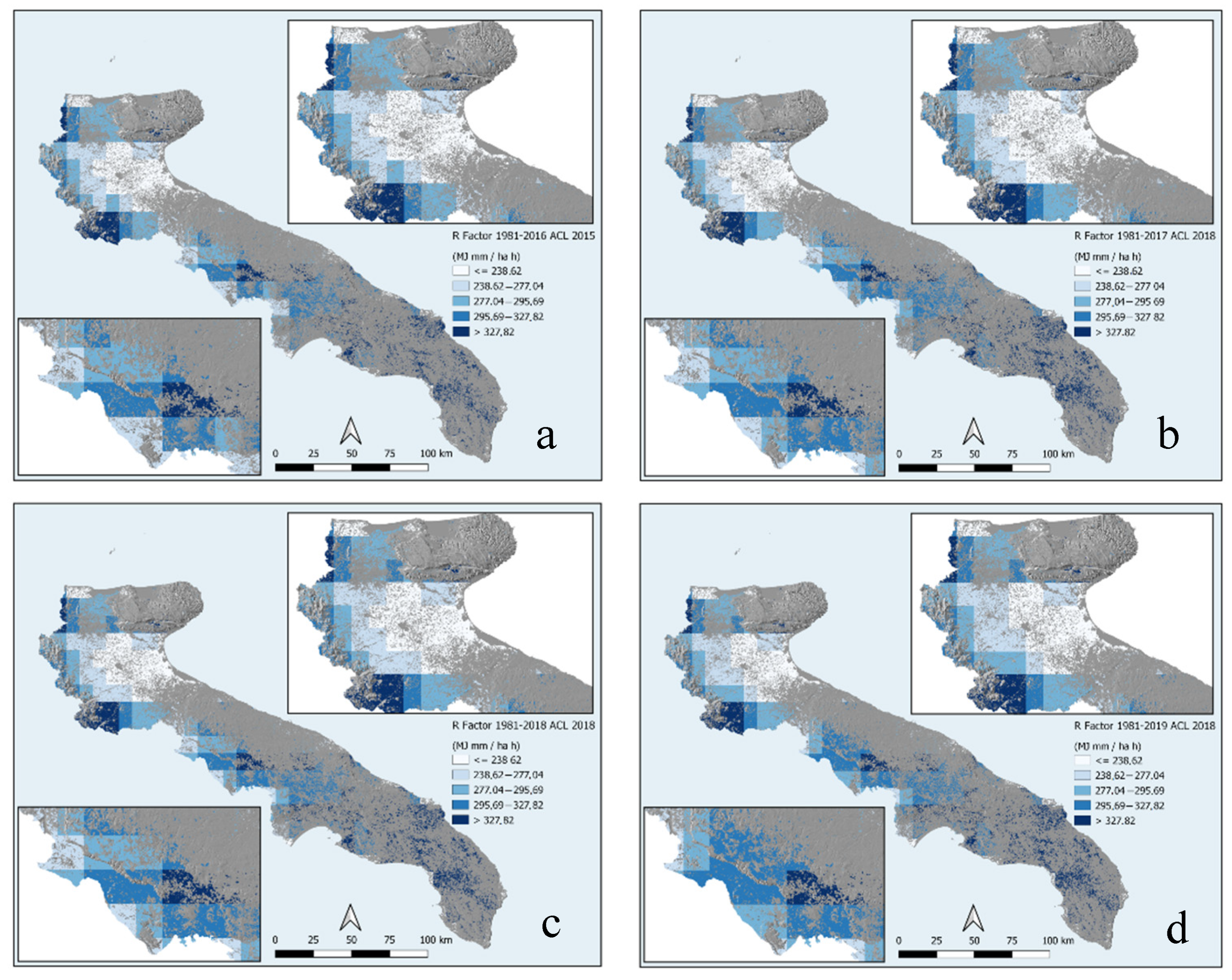
2.2.1. R-Factor
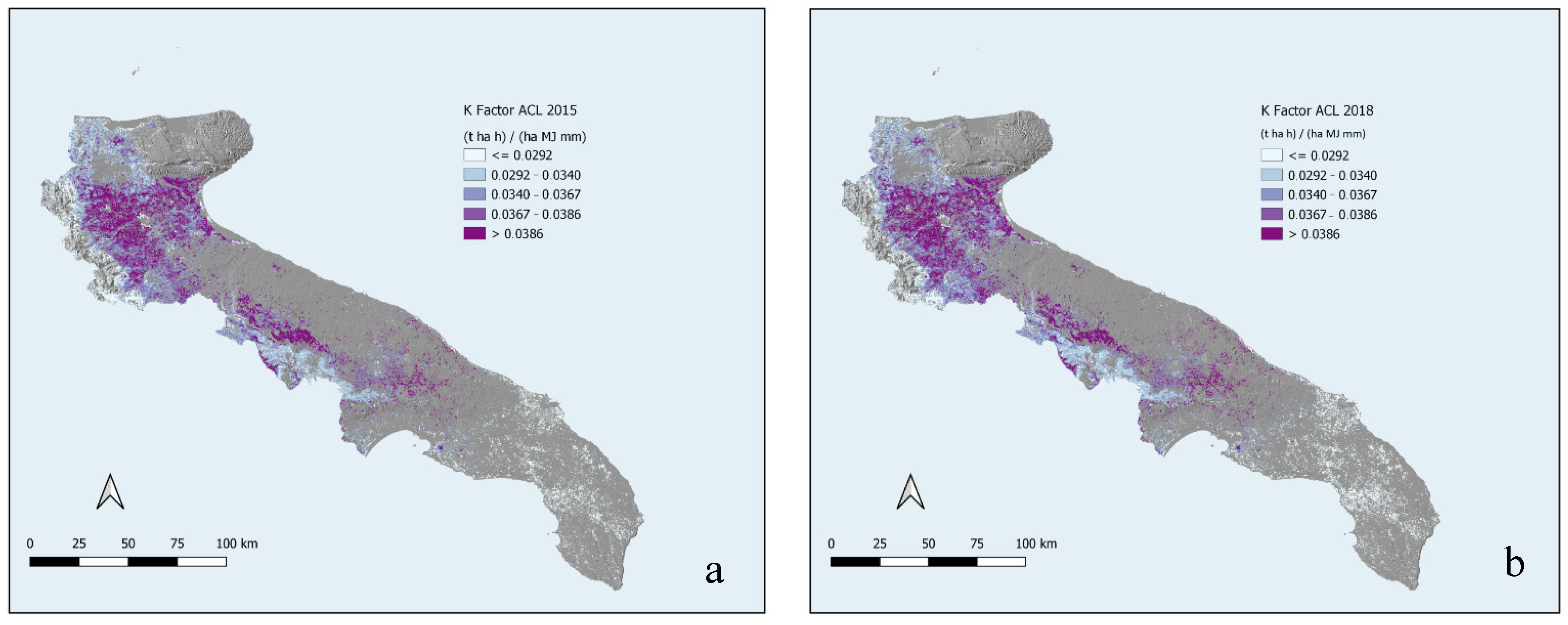
2.2.2. K-Factor
2.2.3. P-Factor
2.2.4. LS-Factor
2.2.5. C-Factor
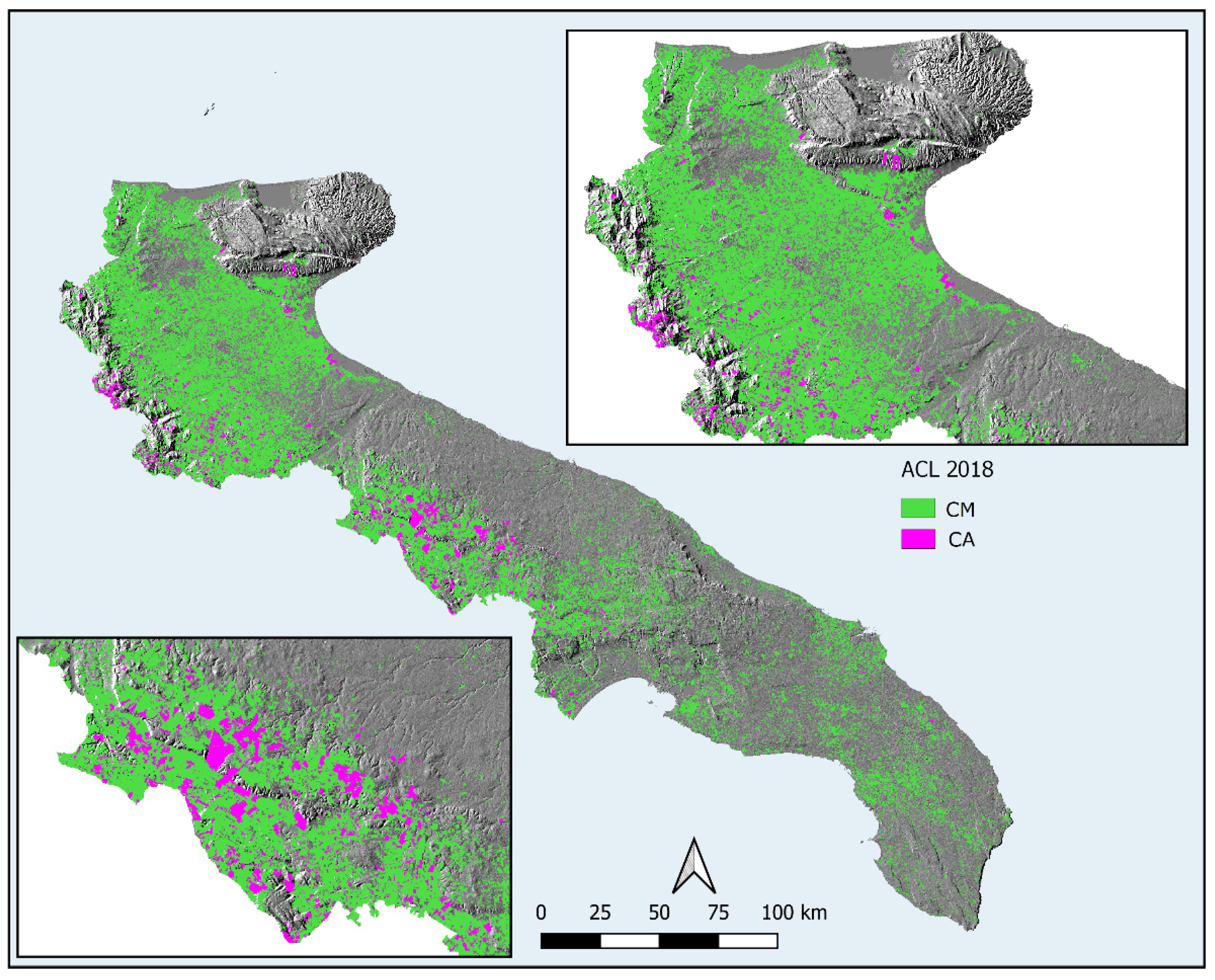
2.3. Identification of ACL
2.4. RUSLE Factors Multiplication
3. Results and Discussion
3.1. Rainfall Erosivity (R-Factor)
3.2. Soil Erodibility (K) and Support Practice Factor (P)
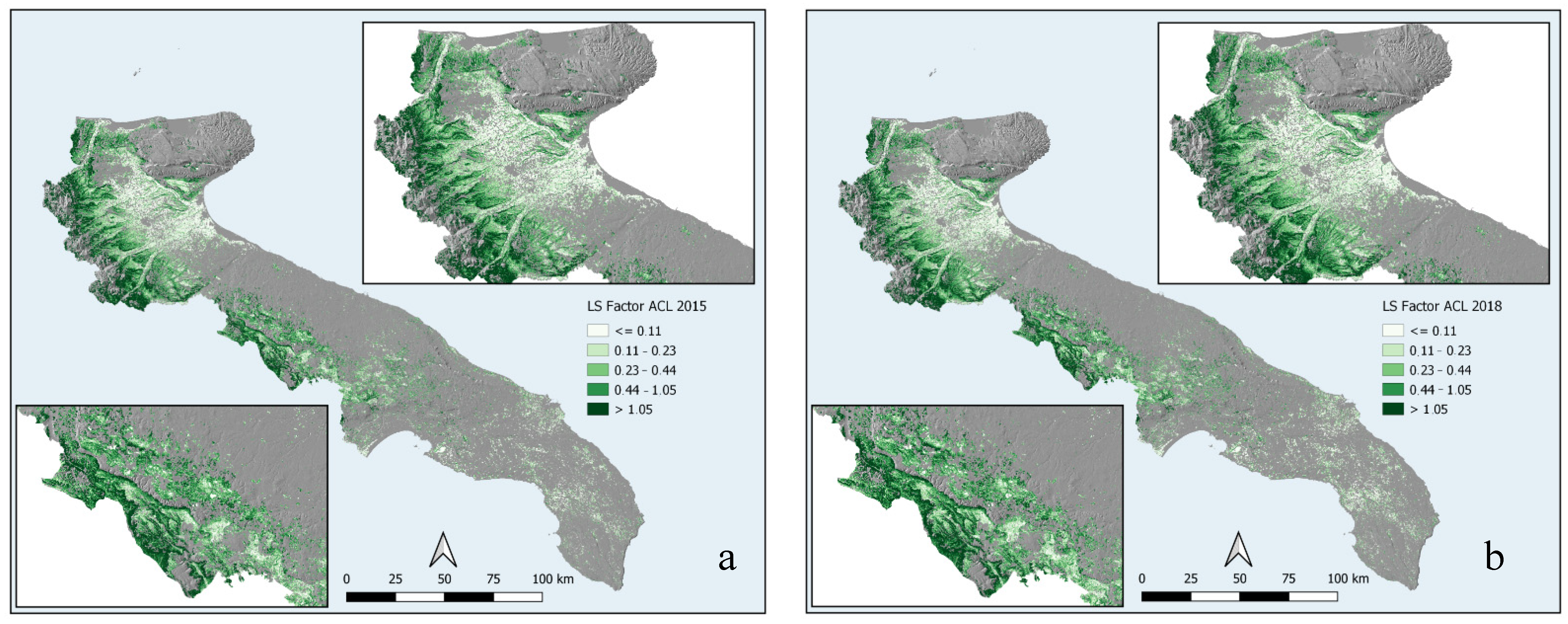
3.3. Topographic Factor (LS)
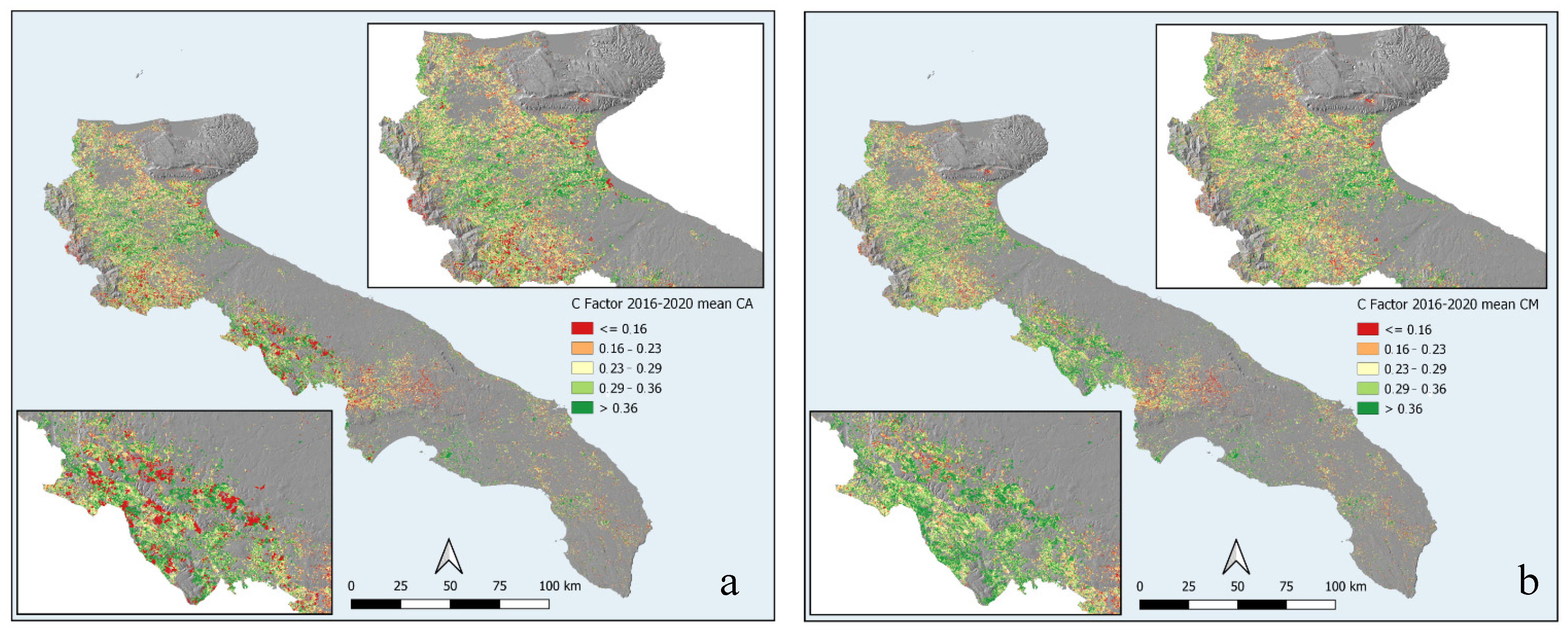
3.4. Cover-Management (C-Factor)
3.5. Soil Loss Estimation in the Apulia Region
3.5.1. Loss Rates
3.5.2. Mean Loss Rates for Altitude and Slope Classes
3.5.3. Combination of Altitude and Slope Classes
4. Conclusions
Supplementary Materials
Author Contributions
Funding
Institutional Review Board Statement
Informed Consent Statement
Data Availability Statement
Acknowledgments
Conflicts of Interest
References
- de la Rosa, D.; Sobral, R. Soil Quality and Methods for its Assessment. In Land Use and Soil Resources; Braimoh, A.K., Vlek, P.L.G., Eds.; Springer: Dordrecht, Netherlands, 2008; pp. 167–200. ISBN 978-1-4020-6778-5. [Google Scholar]
- Pham, T.G.; Nguyen, H.T.; Kappas, M. Assessment of soil quality indicators under different agricultural land uses and topographic aspects in Central Vietnam. Int. Soil Water Conserv. Res. 2018, 6, 280–288. [Google Scholar] [CrossRef]
- Tian, P.; Zhu, Z.; Yue, Q.; He, Y.; Zhang, Z.; Hao, F.; Guo, W.; Chen, L.; Liu, M. Soil erosion assessment by RUSLE with improved P factor and its validation: Case study on mountainous and hilly areas of Hubei Province, China. Int. Soil Water Conserv. Res. 2021, 9, 433–444. [Google Scholar] [CrossRef]
- Bullock, P. CLIMATE CHANGE IMPACTS. In Encyclopedia of Soils in the Environment; Hillel, D., Ed.; Elsevier: Oxford, UK, 2005; pp. 254–262. ISBN 978-0-12-348530-4. [Google Scholar]
- Karlen, D.L.; Mausbach, M.J.; Doran, J.W.; Cline, R.G.; Harris, R.F.; Schuman, G.E. Soil Quality: A Concept, Definition, and Framework for Evaluation (A Guest Editorial). Soil Sci. Soc. Am. J. 1997, 61, 4–10. [Google Scholar] [CrossRef] [Green Version]
- Lal, R. Soil Quality and Soil Erosion; Lal, R., Ed.; CRC Press: Boca Raton, FL, USA, 2018; ISBN 9780203739266. [Google Scholar]
- Pimentel, D. Soil Erosion: A Food and Environmental Threat. Environ. Dev. Sustain. 2006, 8, 119–137. [Google Scholar] [CrossRef]
- Nyakatawa, E.; Jakkula, V.; Reddy, K.; Lemunyon, J.; Norrisjr, B. Soil erosion estimation in conservation tillage systems with poultry litter application using RUSLE 2.0 model. Soil Tillage Res. 2007, 94, 410–419. [Google Scholar] [CrossRef]
- Dale, V.H.; Polasky, S. Measures of the effects of agricultural practices on ecosystem services. Ecol. Econ. 2007, 64, 286–296. [Google Scholar] [CrossRef]
- Dominati, E.; Patterson, M.; Mackay, A. A framework for classifying and quantifying the natural capital and ecosystem services of soils. Ecol. Econ. 2010, 69, 1858–1868. [Google Scholar] [CrossRef]
- Onori, F.; De Bonis, P.; Grauso, S. Soil erosion prediction at the basin scale using the revised universal soil loss equation (RUSLE) in a catchment of Sicily (southern Italy). Environ. Geol. 2006, 50, 1129–1140. [Google Scholar] [CrossRef]
- Van der Knijff, J.M.; Jones, R.J.A.; Montanarella, L. Soil Erosion Risk Assessment in Europe; EUR 19044 EN; Office for Official Publications of the European Communities: Luxemburg, 2000. [Google Scholar]
- McCool, D.K.; Williams, J.D. Soil Erosion by Water. In Encyclopedia of Ecology; Jørgensen, S.E., Fath, B.D., Eds.; Academic Press: Oxford, UK, 2008; pp. 3284–3290. ISBN 978-0-08-045405-4. [Google Scholar]
- Stolte, J.; Tesfai, M.; Øygarden, L.; Kværnø, S.; Keizer, J.; Verheijen, F. Soil Threats in Europe: Status, Methods, Drivers and Effects on Ecosystem. Services: Deliverable 2.1 RECARE Project; European Soil Data Centre, European Union; 2016; Available online: https://esdac.jrc.ec.europa.eu/public_path/shared_folder/doc_pub/EUR27607.pdf (accessed on 1 November 2021).
- Paul, C.; Kuhn, K.; Steinhoff-Knopp, B.; Weißhuhn, P.; Helming, K. Towards a standardization of soil-related ecosystem service assessments. Eur. J. Soil Sci. 2021, 72, 1543–1558. [Google Scholar] [CrossRef]
- Steinhoff-Knopp, B.; Kuhn, T.K.; Burkhard, B. The impact of soil erosion on soil-related ecosystem services: Development and testing a scenario-based assessment approach. Environ. Monit. Assess. 2021, 193, 274. [Google Scholar] [CrossRef]
- Farooq, M.; Pisante, M. Innovations in Sustainable Agriculture; Farooq, M., Pisante, M., Eds.; Springer International Publishing: Cham, Switzerland, 2019; ISBN 978-3-030-23168-2. [Google Scholar]
- Füssel, H.M.; Marx, A.; Hildén, M. Climate Change, Impacts and Vulnerability in Europe 2016—An Indicator-based Report; EEA Report No 1/2017; EEA: Copenhagen, Denmark, 2017. [Google Scholar]
- Jat, R.A.; Kanwar, L.; Sahrawat Amir, H.; Kassam, T.F. Conservation agriculture for sustainable and resilient agriculture: Global status, prospects and challenges. In Conservation Agriculture: Global Prospects and Challenges; CABI Publishing: Wallingford, UK, 2014; pp. 1–25. [Google Scholar]
- Ronco, P.; Zennaro, F.; Torresan, S.; Critto, A.; Santini, M.; Trabucco, A.; Zollo, A.L.; Galluccio, G.; Marcomini, A. A risk assessment framework for irrigated agriculture under climate change. Adv. Water Resour. 2017, 110, 562–578. [Google Scholar] [CrossRef]
- Ferreira, C.S.S.; Seifollahi-Aghmiuni, S.; Destouni, G.; Ghajarnia, N.; Kalantari, Z. Soil degradation in the European Mediterranean region: Processes, status and consequences. Sci. Total Environ. 2022, 805, 150106. [Google Scholar] [CrossRef]
- Preiti, G.; Romeo, M.; Bacchi, M.; Monti, M. Soil loss measure from Mediterranean arable cropping systems: Effects of rotation and tillage system on C-factor. Soil Tillage Res. 2017, 170, 85–93. [Google Scholar] [CrossRef]
- Montanarella, L. Soil Conservation in the European Union; DLG-Verlag GmbH: Frankfurt, Germany, 2013. [Google Scholar]
- Morgan, R.P. Soil Erosion and Conservation; John Wiley & Sons: Hoboken, NJ, USA, 2005; ISBN 978-1-405-14467-4. [Google Scholar]
- Simonneaux, V.; Cheggour, A.; Deschamps, C.; Mouillot, F.; Cerdan, O.; Le Bissonnais, Y. Land use and climate change effects on soil erosion in a semi-arid mountainous watershed (High Atlas, Morocco). J. Arid Environ. 2015, 122, 64–75. [Google Scholar] [CrossRef] [Green Version]
- Bhatt, R.; Kukal, S.S.; Busari, M.A.; Arora, S.; Yadav, M. Sustainability issues on rice–wheat cropping system. Int. Soil Water Conserv. Res. 2016, 4, 64–74. [Google Scholar] [CrossRef] [Green Version]
- Corsi, S.; Friedrich, T.; Kassam, A.; Pisante, M.; Sà, J.D.M. Soil Organic Carbon Accumulation and Greenhouse Gas Emission Reductions from Conservation Agriculture: A Literature Review; Food and Agriculture Organization of the United Nations: Rome, Italy, 2012; Volume 16, ISBN 9789251071878. [Google Scholar]
- González-Sánchez, E.J.; Moreno-García, M.; Kassam, A.; Holgado-Cabrera, A.; Triviño-Tarradas, P.; Carbonell-Bojollo, R.; Pisante, M.; Veroz-González, O.; Basch, G. Conservation Agriculture: Making Climate Change Mitigation and Adaptation Real in Europe; European Conservation Agriculture Federation: Brussels, Belgium, 2017. [Google Scholar]
- Kassam, A. Advances in Conservation Agriculture: Volume 2: Practice and Benefits.; Kassam, A., Ed.; Burleigh Dodds Science Publishing Limited: Cambridge, UK, 2020. [Google Scholar]
- Pisante, M.; Stagnari, F.; Acutis, M.; Bindi, M.; Brilli, L.; Di Stefano, V.; Carozzi, M. Conservation Agriculture and Climate Change. In Conservation Agriculture; Springer International Publishing: Cham, Switzerland, 2015; pp. 579–620. [Google Scholar]
- Sturny, W.G.; Chervet, A.; Maurer-Troxler, C.; Ramseier, L.; Müller, M.; Schafflützel, R.; Richner, W.; Streit, B.; Weisskopf, P.; Zihlmann, U. Comparison of no-tillage and conventional plow tillage—A synthesis. AGRARForschung 2007, 14, 350–357. [Google Scholar]
- Panagos, P.; Ballabio, C.; Poesen, J.; Lugato, E.; Scarpa, S.; Montanarella, L.; Borrelli, P. A Soil Erosion Indicator for Supporting Agricultural, Environmental and Climate Policies in the European Union. Remote Sens. 2020, 12, 1365. [Google Scholar] [CrossRef]
- Cerdan, O.; Govers, G.; Le Bissonnais, Y.; Van Oost, K.; Poesen, J.; Saby, N.; Gobin, A.; Vacca, A.; Quinton, J.; Auerswald, K.; et al. Rates and spatial variations of soil erosion in Europe: A study based on erosion plot data. Geomorphology 2010, 122, 167–177. [Google Scholar] [CrossRef]
- Panagos, P.; Borrelli, P.; Meusburger, K.; Alewell, C.; Lugato, E.; Montanarella, L. Estimating the soil erosion cover-management factor at the European scale. Land Use Policy 2015, 48, 38–50. [Google Scholar] [CrossRef]
- Efthimiou, N.; Psomiadis, E. The Significance of Land Cover Delineation on Soil Erosion Assessment. Environ. Manag. 2018, 62, 383–402. [Google Scholar] [CrossRef]
- Frattaruolo, F.; Pennetta, L.; Piccarreta, M. Desertification Vulnerability Map of Tavoliere, Apulia (Southern Italy). J. Maps 2009, 5, 117–125. [Google Scholar] [CrossRef] [Green Version]
- Ladisa, G.; Todorovic, M.; Trisorio Liuzzi, G. A GIS-based approach for desertification risk assessment in Apulia region, SE Italy. Phys. Chem. Earth Parts A/B/C 2012, 49, 103–113. [Google Scholar] [CrossRef]
- Wang, H.; Zhao, H. Dynamic Changes of Soil Erosion in the Taohe River Basin Using the RUSLE Model and Google Earth Engine. Water 2020, 12, 1293. [Google Scholar] [CrossRef]
- Di Nunno, F.; Granata, F. Groundwater level prediction in Apulia region (Southern Italy) using NARX neural network. Environ. Res. 2020, 190, 110062. [Google Scholar] [CrossRef] [PubMed]
- Serio, F.; Miglietta, P.P.; Lamastra, L.; Ficocelli, S.; Intini, F.; De Leo, F.; De Donno, A. Groundwater nitrate contamination and agricultural land use: A grey water footprint perspective in Southern Apulia Region (Italy). Sci. Total Environ. 2018, 645, 1425–1431. [Google Scholar] [CrossRef] [PubMed]
- Abu Hammad, A. Watershed erosion risk assessment and management utilizing revised universal soil loss equation-geographic information systems in the Mediterranean environments. Water Environ. J. 2011, 25, 149–162. [Google Scholar] [CrossRef]
- Prasannakumar, V.; Shiny, R.; Geetha, N.; Vijith, H. Spatial prediction of soil erosion risk by remote sensing, GIS and RUSLE approach: A case study of Siruvani river watershed in Attapady valley, Kerala, India. Environ. Earth Sci. 2011, 64, 965–972. [Google Scholar] [CrossRef]
- Yesuph, A.Y.; Dagnew, A.B. Soil erosion mapping and severity analysis based on RUSLE model and local perception in the Beshillo Catchment of the Blue Nile Basin, Ethiopia. Environ. Syst. Res. 2019, 8, 17. [Google Scholar] [CrossRef] [Green Version]
- Haregeweyn, N.; Tsunekawa, A.; Poesen, J.; Tsubo, M.; Meshesha, D.T.; Fenta, A.A.; Nyssen, J.; Adgo, E. Comprehensive assessment of soil erosion risk for better land use planning in river basins: Case study of the Upper Blue Nile River. Sci. Total Environ. 2017, 574, 95–108. [Google Scholar] [CrossRef] [Green Version]
- Elnashar, A.; Wang, L.; Wu, B.; Zhu, W.; Zeng, H. Synthesis of global actual evapotranspiration from 1982 to 2019. Earth Syst. Sci. Data 2021, 13, 447–480. [Google Scholar] [CrossRef]
- Tian, F.; Wu, B.; Zeng, H.; Zhang, X.; Xu, J. Efficient Identification of Corn Cultivation Area with Multitemporal Synthetic Aperture Radar and Optical Images in the Google Earth Engine Cloud Platform. Remote Sens. 2019, 11, 629. [Google Scholar] [CrossRef] [Green Version]
- Zeng, H.; Wu, B.; Wang, S.; Musakwa, W.; Tian, F.; Mashimbye, Z.E.; Poona, N.; Syndey, M. A Synthesizing Land-cover Classification Method Based on Google Earth Engine: A Case Study in Nzhelele and Levhuvu Catchments, South Africa. Chin. Geogr. Sci. 2020, 30, 397–409. [Google Scholar] [CrossRef]
- Renard, K.G.; Foster, G.R.; Weesies, G.A.; Porter, J.P. RUSLE: Revised universal soil loss equation. J. Soil Water Conserv. 1991, 46, 30–33. [Google Scholar]
- Renard, K.G. Predicting Soil Erosion by Water: A Guide to Conservation Planning with the Revised Universal Soil Loss Equation (RUSLE); United States Department of Agriculture: Washington, DC, USA, 1997.
- Brown, L.C.; Foster, G.R. Storm Erosivity Using Idealized Intensity Distributions. Trans. ASAE 1987, 30, 379–386. [Google Scholar] [CrossRef]
- Diodato, N. Estimating RUSLE’s rainfall factor in the part of Italy with a Mediterranean rainfall regime. Hydrol. Earth Syst. Sci. 2004, 8, 103–107. [Google Scholar] [CrossRef] [Green Version]
- Wischmeier, W.H.; Smith, D. Predicting Rainfall Erosion Losses: A Guide to Conservation Planning (No. 537); Department of Agriculture, Science and Education Administration: Washington, DC, USA, 1978. [Google Scholar]
- Panagos, P.; Meusburger, K.; Ballabio, C.; Borrelli, P.; Alewell, C. Soil erodibility in Europe: A high-resolution dataset based on LUCAS. Sci. Total Environ. 2014, 479–480, 189–200. [Google Scholar] [CrossRef]
- Tóth, G.; Jones, A.; Montanarella, L. The LUCAS topsoil database and derived information on the regional variability of cropland topsoil properties in the European Union. Environ. Monit. Assess. 2013, 185, 7409–7425. [Google Scholar] [CrossRef]
- Quinlan, J.R. Learning with continuous classes. In Proceedings of the Australian Joint Conference on Artificial Intelligence, Hobart, TAS, Australia, 16–18 November 1992; pp. 343–348. [Google Scholar]
- Panagos, P.; Borrelli, P.; Poesen, J.; Ballabio, C.; Lugato, E.; Meusburger, K.; Montanarella, L.; Alewell, C. The new assessment of soil loss by water erosion in Europe. Environ. Sci. Policy 2015, 54, 438–447. [Google Scholar] [CrossRef]
- Panagos, P.; Borrelli, P.; Meusburger, K.; van der Zanden, E.H.; Poesen, J.; Alewell, C. Modelling the effect of support practices (P-factor) on the reduction of soil erosion by water at European scale. Environ. Sci. Policy 2015, 51, 23–34. [Google Scholar] [CrossRef]
- Panagos, P.; Borrelli, P.; Meusburger, K. A New European Slope Length and Steepness Factor (LS-Factor) for Modeling Soil Erosion by Water. Geosciences 2015, 5, 117–126. [Google Scholar] [CrossRef] [Green Version]
- Desmet, P.J.J.; Govers, G. A GIS procedure for automatically calculating the USLE LS factor on topographically complex landscape units. J. Soil Water Conserv. 1996, 51, 427–433. [Google Scholar]
- Mashimbye, Z.E.; de Clercq, W.P.; Van Niekerk, A. An evaluation of digital elevation models (DEMs) for delineating land components. Geoderma 2014, 213, 312–319. [Google Scholar] [CrossRef]
- Olaya, V.; Conrad, O. Chapter 12 Geomorphometry in SAGA. In Geomorphometry Concepts, Software, Applications, Developments in Soil Science; Hengl, T., Reuter, H.I., Eds.; Elsevier: Amsterdam, The Neatherlands, 2009; pp. 293–308. [Google Scholar]
- Estrada-Carmona, N.; Harper, E.B.; DeClerck, F.; Fremier, A.K. Quantifying model uncertainty to improve watershed-level ecosystem service quantification: A global sensitivity analysis of the RUSLE. Int. J. Biodivers. Sci. Ecosyst. Serv. Manag. 2017, 13, 40–50. [Google Scholar] [CrossRef]
- Nearing, M.A.; Jetten, V.; Baffaut, C.; Cerdan, O.; Couturier, A.; Hernandez, M.; Le Bissonnais, Y.; Nichols, M.H.; Nunes, J.P.; Renschler, C.S.; et al. Modeling response of soil erosion and runoff to changes in precipitation and cover. CATENA 2005, 61, 131–154. [Google Scholar] [CrossRef]
- Almagro, A.; Oliveira, P.T.S.; Nearing, M.A.; Hagemann, S. Projected climate change impacts in rainfall erosivity over Brazil. Sci. Rep. 2017, 7, 8130. [Google Scholar] [CrossRef] [Green Version]
- Buttafuoco, G.; Conforti, M.; Aucelli, P.P.C.; Robustelli, G.; Scarciglia, F. Assessing spatial uncertainty in mapping soil erodibility factor using geostatistical stochastic simulation. Environ. Earth Sci. 2012, 66, 1111–1125. [Google Scholar] [CrossRef]
- Van der Knijff, J.M.F.; Jones, R.J.A.; Montanarella, L. Soil Erosion Risk Assessment in Italy; Office for Official Publications of the European Communities: Luxembourg, 1999. [Google Scholar]
- Durigon, V.L.; Carvalho, D.F.; Antunes, M.A.H.; Oliveira, P.T.S.; Fernandes, M.M. NDVI time series for monitoring RUSLE cover management factor in a tropical watershed. Int. J. Remote Sens. 2014, 35, 441–453. [Google Scholar] [CrossRef]
- Pechanec, V.; Mráz, A.; Benc, A.; Cudlín, P. Analysis of spatiotemporal variability of C-factor derived from remote sensing data. J. Appl. Remote Sens. 2018, 12, 016022. [Google Scholar] [CrossRef]
- Vatandaşlar, C.; Yavuz, M. Modeling cover management factor of RUSLE using very high-resolution satellite imagery in a semiarid watershed. Environ. Earth Sci. 2017, 76, 65. [Google Scholar] [CrossRef]
- Vijith, H.; Seling, L.W.; Dodge-Wan, D. Effect of cover management factor in quantification of soil loss: Case study of Sungai Akah subwatershed, Baram River basin Sarawak, Malaysia. Geocarto Int. 2018, 33, 505–521. [Google Scholar] [CrossRef]
- Main-Knorn, M.; Pflug, B.; Louis, J.; Debaecker, V.; Müller-Wilm, U.; Gascon, F. Sen2Cor for Sentinel-2. In Proceedings SPIE 10427, Image and Signal Processing for Remote Sensing XXIII; Bruzzone, L., Bovolo, F., Benediktsson, J.A., Eds.; SPIE: Warsaw, Poland, 2017; p. 3. [Google Scholar]
- Hadjimitsis, D.G.; Papadavid, G.; Agapiou, A.; Themistocleous, K.; Hadjimitsis, M.G.; Retalis, A.; Michaelides, S.; Chrysoulakis, N.; Toulios, L.; Clayton, C.R.I. Atmospheric correction for satellite remotely sensed data intended for agricultural applications: Impact on vegetation indices. Nat. Hazards Earth Syst. Sci. 2010, 10, 89–95. [Google Scholar] [CrossRef] [Green Version]
- Sola, I.; Alvarez-Mozos, J.; Gonzalez-Audicana, M. Inter-Comparison of Atmospheric Correction Methods on Sentinel-2 Images Applied to Croplands. In Proceedings of the IGARSS 2018—2018 IEEE International Geoscience and Remote Sensing Symposium, Valencia, Spain, 22–27 July 2018; pp. 5940–5943. [Google Scholar]
- Alexakis, D.D.; Manoudakis, S.; Agapiou, A.; Polykretis, C. Towards the Assessment of Soil-Erosion-Related C-Factor on European Scale Using Google Earth Engine and Sentinel-2 Images. Remote Sens. 2021, 13, 5019. [Google Scholar] [CrossRef]
- Gallego, J.; Bamps, C. Using CORINE land cover and the point survey LUCAS for area estimation. Int. J. Appl. Earth Obs. Geoinf. 2008, 10, 467–475. [Google Scholar] [CrossRef]
- D’Andrimont, R.; Yordanov, M.; Martinez-Sanchez, L.; Eiselt, B.; Palmieri, A.; Dominici, P.; Gallego, J.; Reuter, H.I.; Joebges, C.; Lemoine, G.; et al. Harmonised LUCAS in-situ land cover and use database for field surveys from 2006 to 2018 in the European Union. Sci. Data 2020, 7, 352. [Google Scholar] [CrossRef]
- Buchhorn, M.; Smets, B.; Bertels, L.; De Roo, B.; Lesiv, M.; Tsendbazar, N.E.; Herold, M.F. Copernicus Global Land Service: Land Cover 100m: Collection 3: Epoch 2015: Globe (Version V3.0.1). Available online: https://zenodo.org/record/3939038#.YZz08WDMK5c (accessed on 1 November 2021).
- Buchhorn, M.; Smets, B.; Bertels, L.; De Roo, B.; Lesiv, M.; Tsendbazar, N.E.; Herold, M.F. Copernicus Global Land Service: Land Cover 100m: Collection 3: Epoch 2018: Globe (Version V3.0.1). Available online: https://zenodo.org/record/3518038#.YZz0V2DMK5c (accessed on 1 November 2021).
- Gorelick, N.; Hancher, M.; Dixon, M.; Ilyushchenko, S.; Thau, D.; Moore, R. Google Earth Engine: Planetary-scale geospatial analysis for everyone. Remote Sens. Environ. 2017, 202, 18–27. [Google Scholar] [CrossRef]
- Borrelli, P.; Diodato, N.; Panagos, P. Rainfall erosivity in Italy: A national scale spatio-temporal assessment. Int. J. Digit. Earth 2016, 9, 835–850. [Google Scholar] [CrossRef] [Green Version]
- Panagos, P.; Ballabio, C.; Borrelli, P.; Meusburger, K.; Klik, A.; Rousseva, S.; Tadić, M.P.; Michaelides, S.; Hrabalíková, M.; Olsen, P.; et al. Rainfall erosivity in Europe. Sci. Total Environ. 2015, 511, 801–814. [Google Scholar] [CrossRef] [Green Version]
- Ayalew, D.A.; Deumlich, D.; Šarapatka, B. Agricultural landscape-scale C factor determination and erosion prediction for various crop rotations through a remote sensing and GIS approach. Eur. J. Agron. 2021, 123, 126203. [Google Scholar] [CrossRef]
- Panagos, P.; Meusburger, K.; Van Liedekerke, M.; Alewell, C.; Hiederer, R.; Montanarella, L. Assessing soil erosion in Europe based on data collected through a European network. Soil Sci. Plant. Nutr. 2014, 60, 15–29. [Google Scholar] [CrossRef] [Green Version]
- Bircher, P.; Liniger, H.P.; Prasuhn, V. Comparing different multiple flow algorithms to calculate RUSLE factors of slope length (L) and slope steepness (S) in Switzerland. Geomorphology 2019, 346, 106850. [Google Scholar] [CrossRef]
- Hickey, R. Slope Angle and Slope Length Solutions for GIS. Cartography 2000, 29, 1–8. [Google Scholar] [CrossRef]
- Kienzle, S. The Effect of DEM Raster Resolution on First Order, Second Order and Compound Terrain Derivatives. Trans. GIS 2004, 8, 83–111. [Google Scholar] [CrossRef]
- Thompson, J.A.; Bell, J.C.; Butler, C.A. Digital elevation model resolution: Effects on terrain attribute calculation and quantitative soil-landscape modeling. Geoderma 2001, 100, 67–89. [Google Scholar] [CrossRef]
- Ayalew, D.A.; Deumlich, D.; Šarapatka, B.; Doktor, D. Quantifying the Sensitivity of NDVI-Based C Factor Estimation and Potential Soil Erosion Prediction using Spaceborne Earth Observation Data. Remote Sens. 2020, 12, 1136. [Google Scholar] [CrossRef] [Green Version]
- Borrelli, P.; Robinson, D.A.; Panagos, P.; Lugato, E.; Yang, J.E.; Alewell, C.; Wuepper, D.; Montanarella, L.; Ballabio, C. Land use and climate change impacts on global soil erosion by water (2015–2070). Proc. Natl. Acad. Sci. USA 2020, 117, 21994–22001. [Google Scholar] [CrossRef]
- Märker, M.; Angeli, L.; Bottai, L.; Costantini, R.; Ferrari, R.; Innocenti, L.; Siciliano, G. Assessment of land degradation susceptibility by scenario analysis: A case study in Southern Tuscany, Italy. Geomorphology 2008, 93, 120–129. [Google Scholar] [CrossRef]
- Bargiel, D.; Herrmann, S.; Jadczyszyn, J. Using high-resolution radar images to determine vegetation cover for soil erosion assessments. J. Environ. Manag. 2013, 124, 82–90. [Google Scholar] [CrossRef]
- Almagro, A.; Thomé, T.C.; Colman, C.B.; Pereira, R.B.; Marcato Junior, J.; Rodrigues, D.B.B.; Oliveira, P.T.S. Improving cover and management factor (C-factor) estimation using remote sensing approaches for tropical regions. Int. Soil Water Conserv. Res. 2019, 7, 325–334. [Google Scholar] [CrossRef]
- Lunetta, R.S.; Knight, J.F.; Ediriwickrema, J.; Lyon, J.G.; Worthy, L.D. Land-cover change detection using multi-temporal MODIS NDVI data. Remote Sens. Environ. 2006, 105, 142–154. [Google Scholar] [CrossRef]
- Borrelli, P.; Meusburger, K.; Ballabio, C.; Panagos, P.; Alewell, C. Object-oriented soil erosion modelling: A possible paradigm shift from potential to actual risk assessments in agricultural environments. L Degrad. Dev. 2018, 29, 1270–1281. [Google Scholar] [CrossRef]
- Yan, H.; Wang, L.; Wang, T.W.; Wang, Z.; Shi, Z.H. A synthesized approach for estimating the C-factor of RUSLE for a mixed-landscape watershed: A case study in the Gongshui watershed, southern China. Agric. Ecosyst. Environ. 2020, 301, 107009. [Google Scholar] [CrossRef]
- Lal, R.; Reicosky, D.C.; Hanson, J.D. Evolution of the plow over 10,000 years and the rationale for no-till farming. Soil Tillage Res. 2007, 93, 1–12. [Google Scholar] [CrossRef]
- Ruisi, P.; Giambalvo, D.; Saia, S.; Di Miceli, G.; Frenda, A.S.; Plaia, A.; Amato, G. Conservation tillage in a semiarid Mediterranean environment: Results of 20 years of research. Ital. J. Agron. 2014, 9, 1–7. [Google Scholar] [CrossRef] [Green Version]
- Veihe, A.; Hasholt, B.; Schiøtz, I.G. Soil erosion in Denmark: Processes and politics. Environ. Sci. Policy 2003, 6, 37–50. [Google Scholar] [CrossRef]
- Borrelli, P.; Robinson, D.A.; Fleischer, L.R.; Lugato, E.; Ballabio, C.; Alewell, C.; Meusburger, K.; Modugno, S.; Schütt, B.; Ferro, V.; et al. An assessment of the global impact of 21st century land use change on soil erosion. Nat. Commun. 2017, 8, 2013. [Google Scholar] [CrossRef] [Green Version]
- Borrelli, P.; Paustian, K.; Panagos, P.; Jones, A.; Schütt, B.; Lugato, E. Effect of Good Agricultural and Environmental Conditions on erosion and soil organic carbon balance: A national case study. Land Use Policy 2016, 50, 408–421. [Google Scholar] [CrossRef]
- Panagos, P.; Ballabio, C.; Himics, M.; Scarpa, S.; Matthews, F.; Bogonos, M.; Poesen, J.; Borrelli, P. Projections of soil loss by water erosion in Europe by 2050. Environ. Sci. Policy 2021, 124, 380–392. [Google Scholar] [CrossRef]


| Agricultural Seasons | Images (n) | Mean of NDVI (15/10–01/08) | Cfactor CM | Cfactor CA | % |
|---|---|---|---|---|---|
| 2016–2017 | 309 | 0.3653 | 0.3268 | 0.3122 | −4.5 |
| 2017–2018 | 415 | 0.3995 | 0.2742 | 0.2623 | −4.3 |
| 2018–2019 | 408 | 0.3985 | 0.2803 | 0.2684 | −4.2 |
| 2019–2020 | 449 | 0.4078 | 0.2656 | 0.2552 | −3.9 |
| Mean | 0.3928 | 0.2867 | 0.2745 | −4.2 |
| RUSLE | |||
|---|---|---|---|
| CM | CA | ||
| Agricultural Seasons 2016–2020 | t ha−1 | t ha−1 | Δ% |
| Mean | 2.28 | 2.11 | −7.5 |
| RUSLE | ||||||||||||||||
|---|---|---|---|---|---|---|---|---|---|---|---|---|---|---|---|---|
| Agricultural Seasons |  | 2016–2017 | 2017–2018 | 2018–2019 | 2019–2020 | |||||||||||
| Total Annual Crops Area 2015 | CM | CA | Δ% | Total Annual Crops Area 2018 | CM | CA | Δ% | CM | CA | Δ% | CM | CA | Δ% | Means Δ% | ||
| Numerical Class | Altitude Class | % | t ha−1 y−1 | t ha−1 y−1 | % | % | t ha−1 y−1 | t ha−1 y−1 | % | t ha−1 y−1 | t ha−1 y−1 | % | t ha−1 y−1 | t ha−1 y−1 | % | % |
| 100 | Plain | 67.56 | 1.57 | 1.50 | −4.5 | 68.23 | 1.14 | 1.09 | −4.4 | 1.35 | 1.32 | −2.2 | 1.31 | 1.26 | −3.8 | −3.7 |
| 200 | Hilly | 31.86 | 4.03 | 3.63 | −9.9 | 31.33 | 2.78 | 2.51 | −9.7 | 3.55 | 3.15 | −11.3 | 2.91 | 2.63 | −9.6 | −10.1 |
| 300 | Mountain | 0.58 | 4.89 | 4.01 | −18 | 0.44 | 2.72 | 2.45 | −9.9 | 2.82 | 2.88 | 2.1 | 2.92 | 2.63 | −9.9 | −8.9 |
| 1 | Low slope | 29.25 | 0.64 | 0.61 | −4.7 | 29.79 | 0.45 | 0.42 | −6.7 | 0.55 | 0.53 | −3.6 | 0.53 | 0.51 | −3.8 | −4.7 |
| 2 | Medium slope | 33.50 | 0.79 | 0.75 | −5.1 | 34.15 | 0.55 | 0.52 | −5.5 | 0.68 | 0.65 | −4.4 | 0.64 | 0.61 | −4.7 | −4.9 |
| 3 | High slope | 37.25 | 3.80 | 3.50 | −7.9 | 35.99 | 2.69 | 2.49 | −7.4 | 3.32 | 3.06 | −7.8 | 2.92 | 2.71 | −7.2 | −7.6 |
| 101 | Plain + low slope | 24.67 | 0.65 | 0.63 | −3.1 | 25.19 | 0.56 | 0.55 | −1.8 | 0.66 | 0.57 | −13.6 | 0.57 | 0.56 | −1.8 | −5.1 |
| 102 | Plain + medium slope | 24.93 | 0.79 | 0.77 | −2.5 | 25.47 | 0.47 | 0.45 | −4.3 | 0.56 | 0.57 | 1.8 | 0.57 | 0.56 | −1.8 | −1.7 |
| 103 | Plain + high slope | 17.94 | 3.10 | 2.96 | −4.5 | 17.54 | 1.98 | 1.90 | −4 | 2.37 | 2.27 | −4.2 | 2.24 | 2.15 | −4 | −4.2 |
| 201 | Hilly + low slope | 4.51 | 1.07 | 0.97 | −9.3 | 4.60 | 0.78 | 0.71 | −9 | 1.08 | 0.77 | −28.7 | 0.74 | 0.67 | −9.5 | −14.1 |
| 202 | Hilly + medium slope | 8.56 | 1.31 | 1.18 | −9.9 | 8.68 | 0.82 | 0.74 | −9.8 | 1.12 | 0.90 | −19.6 | 0.86 | 0.78 | −9.3 | −12.2 |
| 203 | Hilly + high slope | 18.75 | 5.66 | 5.11 | −9.7 | 18.03 | 3.67 | 3.31 | −9.8 | 4.67 | 4.17 | −10.7 | 3.84 | 3.48 | −9.4 | −9.9 |
| 301 | Mountain + low slope | 0.00 | 1.21 | 0.88 | −27.3 | 0.00 | 1.28 | 1.05 | −18 | 1.25 | 1.12 | −10.4 | 1.34 | 1.08 | −19.4 | −18.8 |
| 302 | Mountain + medium slope | 0.01 | 1.43 | 1.11 | −22.4 | 0.01 | 0.46 | 0.40 | −13 | 0.49 | 0.47 | −4.1 | 0.50 | 0.43 | −14 | −13.4 |
| 303 | Mountain + high slope | 0.56 | 5.89 | 4.84 | −17.8 | 0.43 | 2.74 | 2.47 | −9.9 | 2.85 | 2.90 | 1.8 | 2.94 | 2.65 | −9.9 | −8.9 |
Publisher’s Note: MDPI stays neutral with regard to jurisdictional claims in published maps and institutional affiliations. |
© 2022 by the authors. Licensee MDPI, Basel, Switzerland. This article is an open access article distributed under the terms and conditions of the Creative Commons Attribution (CC BY) license (https://creativecommons.org/licenses/by/4.0/).
Share and Cite
Petito, M.; Cantalamessa, S.; Pagnani, G.; Degiorgio, F.; Parisse, B.; Pisante, M. Impact of Conservation Agriculture on Soil Erosion in the Annual Cropland of the Apulia Region (Southern Italy) Based on the RUSLE-GIS-GEE Framework. Agronomy 2022, 12, 281. https://doi.org/10.3390/agronomy12020281
Petito M, Cantalamessa S, Pagnani G, Degiorgio F, Parisse B, Pisante M. Impact of Conservation Agriculture on Soil Erosion in the Annual Cropland of the Apulia Region (Southern Italy) Based on the RUSLE-GIS-GEE Framework. Agronomy. 2022; 12(2):281. https://doi.org/10.3390/agronomy12020281
Chicago/Turabian StylePetito, Matteo, Silvia Cantalamessa, Giancarlo Pagnani, Francesco Degiorgio, Barbara Parisse, and Michele Pisante. 2022. "Impact of Conservation Agriculture on Soil Erosion in the Annual Cropland of the Apulia Region (Southern Italy) Based on the RUSLE-GIS-GEE Framework" Agronomy 12, no. 2: 281. https://doi.org/10.3390/agronomy12020281
APA StylePetito, M., Cantalamessa, S., Pagnani, G., Degiorgio, F., Parisse, B., & Pisante, M. (2022). Impact of Conservation Agriculture on Soil Erosion in the Annual Cropland of the Apulia Region (Southern Italy) Based on the RUSLE-GIS-GEE Framework. Agronomy, 12(2), 281. https://doi.org/10.3390/agronomy12020281