Article

Mapping Ecological Focus Areas within the EU CAP Controls Framework by Copernicus Sentinel-2 Data

by
Filippo Sarvia
*,
Samuele De Petris
and
Enrico Borgogno-Mondino
Department of Agriculture, Forest and Food Sciences of Torino University, Largo Braccini 2, 10095 Grugliasco, Italy
*
Author to whom correspondence should be addressed.
Agronomy 2022, 12(2), 406; https://doi.org/10.3390/agronomy12020406
Submission received: 22 December 2021 / Revised: 31 January 2022 / Accepted: 4 February 2022 / Published: 6 February 2022

Abstract

:
Greening is a Common Agricultural Policy (CAP) subsidy that ensures that all EU farmers receiving income support produce climate and environmental benefits as part of their farming activities. To receive greening support, it is mandatory for the farmer to carry out three agricultural practices that are considered environmentally and climate friendly: (a) crop diversification; (b) maintenance of permanent meadows and pastures; and (c) presence of an Ecological Focus Area (EFA). Contributions are delivered and monitored by paying agencies (PP) that ordinarily perform administrative checks and spot checks. The latter are provided through photo-interpretation of high-resolution satellite or aerial images and, in specific cases, through local ground checks (GC) as well. In this work, stimulated by the Piemonte Regional Agency for Payments in Agriculture (ARPEA), a prototype service to support PPs’ controls within the greening CAP framework was proposed with special concern for EFA detection. The proposed approach is expected to represent a valid alternative or supporting tool for GC. It relies on the analysis of NDVI time series derived from Copernicus Sentinel-2 data. The study was conducted in the provinces of Turin, Asti and Vercelli within the Piedmont Region (NW Italy), and over 12,500 EFA fields were assessed. Since the recent National Report No. 5465 stipulates that mowing and any other soil management operation is prohibited on set-aside land designated as an EFA during the reference period (RP) between 1st March and 30th June, a time series (TS) of NDVI in the same period was generated. Once averaged at plot level, NDVI trends were modelled by a first-order polynomial, and the correspondent statistics (namely, R2, MAE and maximum residual) was computed. These were assumed to play the role of discriminants in EFA detection based on a thresholding approach (Otsu’s method), calibrated with reference to the training dataset. The threshold satisfaction was therefore tested, and, depending on the number of satisfied thresholds out of the possible three, EFA and non-EFA plots were detected with a different degree of reliability. The correspondent EFA map was generated for the area of interest and validated according to GCs as provided by the ARPEA. The results showed an overall accuracy of 84%, indicating that the approach is promising. The authors retain that this procedure represents a valid alternative (or integrating) tool for ground controls by PPs.

1. Introduction

1.1. Ecological Focus Areas within CAP

Common Agricultural Policy (CAP) is one of the most important EU strategies, receiving around 35% of the European Union (EU) budget. CAP aims to support farmers with contributions to ensure safe and quality food at affordable prices; to protect the farming sector from excessive price volatility, market crises and imbalances affecting the food supply chain; to maintain rural communities across the EU by preserving the environment, animal welfare and biodiversity; to mitigate climate change effects in need of sustainable use of environmental resources [1,2,3]. Many habitats promoting biodiversity rely on agricultural farming systems. Unfortunately, biodiversity protection efforts have no explicit economic value that markets can take into account, making the prices paid to farmers noncomprehensive of related costs [4]. Biodiversity safeguarding depends on appropriate management practices that must continuously change under competitive pressures that determine increasing levels of specialisation and intensification of production, in some cases, and land abandonment in others. These two combined factors impact the biodiversity, which generates detrimental effects on the soil, water and climate, and ultimately threatens the long-term productive potential of the whole agricultural sector.
To limit this trend, in 2015, a new type of CAP subsidy, called “greening”, was introduced [5,6] for EU countries. The basic underlying idea is that agriculture can greatly contribute to reducing the risk of environmental degradation and to mitigating climate change effects. Greening measures are expected to push EU farmers to generate climate and environmental benefits as part of their ordinary farming activities (https://ec.europa.eu/, accessed on 2 February 2022). From this point of view, farmers are seen as important players in environmental safeguarding (biodiversity, landscape, air, water and soil quality, climate stability, greenhouse gas reduction and carbon storage, as well as soil protection from erosion) [6,7,8].
Next, CAP 2023–2027 will include greening as a compulsory practice of conditionality [9,10] with no optional action from farmers. Greening contribution can be obtained if farmers provide evidence of the following three agricultural practices, which are considered environmentally and climate compliant: (a) crop diversification; (b) maintenance of permanent meadows and pastures; (c) existence of an Ecological Focus Area (EFA). According to National Report No. 5465 [11] and Regulation No. 1307/2013 of the European Parliament and Council, Italy requires that farm companies sizing more than 15 hectares must allocate at least 5% of their arable land as an EFA.
The three above-mentioned practices must be jointly applied. An administrative sanction is applied if farmers do not respect these requirements (Article 77(6), EU Regulation No. 1306/2013). This consists of a reduction in the amount of CAP contributions defined by the EU Regulation No. 1307/2013, namely -25% of the basic payment and a complete loss of the greening contribution [12].
The role of EFAs has also been widely discussed at the European level [13]; in fact each member state can define its proper EFA type by selecting them from a common EU list. These criteria apply only to arable land; permanent crops, meadows and/or pastures are not accounted for [14]. In Italy, the following areas are considered an EFA: (a) land lying fallow; (b) terraces; (c) landscape features (hedges, isolated trees, ditches, etc.); (d) buffer strips; (e) agroforestry areas; (f) strip along forest; (g) short rotation coppice; (h) afforested areas; (i) catch crops; and (l) nitrogen-fixing crops. Furthermore, according to Italian regulations, mowing and any other soil management operations are prohibited on set-aside land used as an EFA in the period between 1 March and 30 June (hereinafter called reference period (RP)).
Since CAP support is provided for all EU member states, it is difficult to believe that the payment of contributions can be centralised. Consequently, payment management is demanded by the member states. In Italy, this task is achieved by the regional paying agencies (PP) for some administrative regions and directly by the national one (AGEA) for the others.
Since 2018, according to Article 17 of EU Regulation No. 809/2014, farmers are called to apply for the CAP contribution by submitting the so-called Geo Spatial Aid Application (GSAA). The GSAA contains an actual map of the managed fields and refers to local crop types. A unique identification code is associated with a parcel, making an effective management of CAP applications possible by GIS (Geographic Information System)-based systems [15]. PPs are called to verify the truthfulness of declarations from farmers. Ordinarily, controls are operated with reference to the Integrated Management and Control System (IACS), which includes: (a) administrative controls (AC) for all received applications, aimed at verifying the eligibility of an application and the properness of the supplied documentation, as well as (b) spot controls (SC) that are required for a small subset (5%) of received applications to verify the truthfulness of the submitted information and to test the compliance of farming companies with CAP requirements. Controlled fields are selected according to risk (80%) and randomness (20%) criteria. Generally, SCs are achieved via photo-interpretation of very high-resolution satellite or aerial images; only in particular cases are ground controls (GC) operated.

1.2. Copernicus Satellite Data in the EFA Controls Context

Since 2014, Copernicus Sentinel-1 (S1) and Sentinel-2 (S2) satellites have been providing free high-frequency and high-resolution images. These satellite images represent a potential breakthrough for monitoring agricultural activities at the global scale [16,17]. Specifically, S2 images can be used to derive various spectral indices (e.g., the Normalized Difference Vegetation Index, NDVI), which is useful for providing valuable vegetation-related information [18,19]. S2 data are well known in the literature to be useful for: monitoring vegetation physiology [20,21], estimating crop production [22,23,24], characterising ecosystems [25,26], estimating crop damage from hazardous events for insurance purposes [27,28], assessing tree stability [29], managing private and public forests [30], supporting precision agriculture [31,32] and land cover/use mapping [33,34,35,36], monitoring disaster events [37,38], as well as, recently, for supporting CAP controls in agriculture [39,40,41] (see EU Regulation No. 809/2014 Article 40 bis amended by EU Regulation No. 746/2018). Precisely for this last reason, several member states are working to include Copernicus data in their monitoring procedures.
The recent Italian National Report No. 5465, which applies EU Regulation No. 1307/2013 of the European Parliament and Council, references that mowing and any other soil management operation is prohibited on set-aside land designated as an EFA during RP. Currently, EFA controls can only be achieved through GCs. Being that GCs are highly expensive for PPs, they can only be performed on a small subset of the GSAA, leaving a high probability that false applications remain unknown. In this framework, S2 data are expected to play an important and improving role; they appear to be a valid and operational tool for supporting EFA controls.
It is worthwhile to remember that EFA definition does not depend on crop type; conversely, EFA fields can be, practically, assumed similar to fallow fields since, during the growing season, farmers cannot manage them. Consequently, EFA phenological behaviour is expected to show a progressively increasing NDVI profile with no significant variations due to possible agronomic actions, such as mowing, sowing or harvesting [42]. The period of the year in which this trend must be tested depends on both agronomic calendars and national regulations that, partially, already heed local agronomic calendars, themselves.
Presently, the literature appears to lack works that deal with EFA mapping by satellite in the CAP controls framework, making this work desirable.

1.3. Goals

According to the above-mentioned scenario, in this paper, a prototype procedure based on S2 imagery is proposed to support the EFA controls in Piemonte (NW Italy). It was developed within the framework of an institutional collaboration between the GEO4Agri Lab of the Department of Agricultural, Forest and Food Sciences (DISAFA) of the University of Torino and the Regional Agency for Payments in Agriculture (ARPEA).
The ARPEA explicitly required that the approach was compliant with actual operational scenarios and the available skills that an ordinary regional technician is expected to possess. In other words, it required that the eventual tool for EFA detection was simple enough and explicit in its agronomical meaning, in order to guarantee a conscious utilization and a critical approach to EFA controls. The problem of EFA detection is a typical land cover classification one that is expected to be faced when using satellite data [43]. The above-mentioned requirements from the ARPEA drove the authors to exclude adoption of machine/deep learning-based (MDL) approaches [44,45] and opt for a simpleR rule-based approach, where defined rules could be immediately agronomically interpreted. Moving towards MDL would make it difficult to interpret eventual classification criticalities and, consequently, to properly adjust the algorithm parameters that, in MDL, cannot be related to tangible factors close to the knowledge domain to which the ideal user of the system would belong. Consequently, the proposed approach aims to detect an EFA by applying simple rules, or tasks, to disaggregate a complex problem into a succession of simple and more controllable ones, whereby domain knowledge plays a crucial role in improving classification results.
In this paper, with reference to the study area (see next section), we propose a classification method for EFA detection based on the at-field level analysis of the local NDVI profile from Sentinel-2 imagery. With reference to auxiliary data and ground observations from the ARPEA, we defined simple rules to apply to proper statistics, obtainable from the local NDVI profile. The proposed classification process proceeds by testing the satisfaction of some conditions, which makes it possible to recognize EFAs with acceptable accuracy and, in the meantime, assign a degree of reliability of detection. After validating the results, a map of EFAs was generated for the 2021 year.

2. Materials and Methods
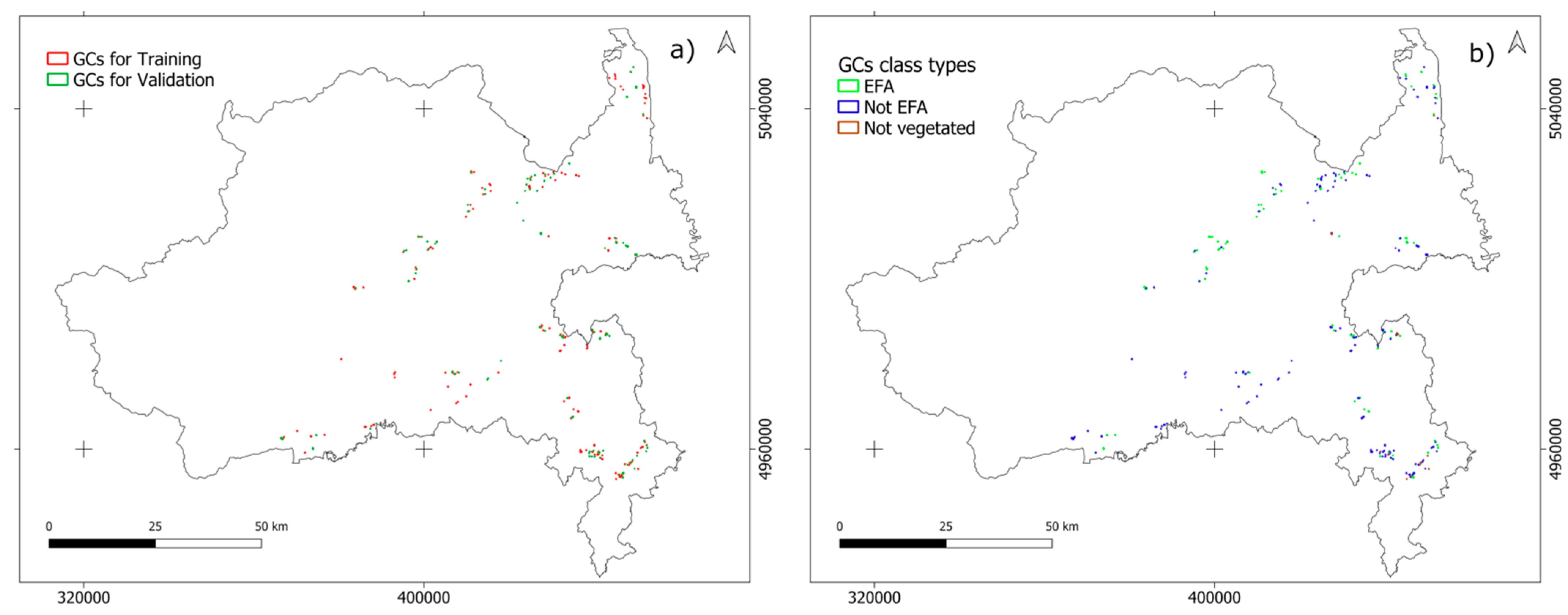
2.1. Study Area

The study area (AOI) includes 3 administrative provinces of the Piemonte region (NW - Italy): namely, Torino, Asti and the southern part of Vercelli (Figure 1). The AOI is located at an altitude ranging between 200 and 300 m a.s.l., covering about 9636 km2. It is characterized by a highly diversified agricultural context, hosting many EFAs. This made it particularly attractive to the ARPEA, as it is called yearly to control the truthfulness of the declared EFAs.

2.2. Available Data

In this work, the following data were used: (a) satellite multispectral images from the Copernicus Sentinel-2 Multi Spectral Instrument (MSI) sensor; (b) maps of the Ecological Focus Area as reported by farmers in the GSAA (year 2021); and (c) calibration and validation data from ground campaigns.

2.2.1. Satellite Data

A total of 43 Level 2A images were collected covering the period from 28 February to 30 June 2021. Level 2A images are BOA (at-the-bottom of the atmosphere) reflectance-calibrated, which is proper for land applications [46,47]. The images were obtained from the Copernicus Open Access Hub geoportal (scihub.copernicus.eu) and provided as 100 km × 100 km tiles orthoprojected in the WGS84 UTM 32N reference system. Red (band 4) and NIR (band 8) bands were used to compute the corresponding Normalized Difference Vegetation Index (NDVI) maps [48]. These have a geometric and temporal resolution of 10 m and 5 days, respectively. The S2 Level 2A dataset is supplied together with an additional band called the “scene classification layer” (SCL), which assigns a classification meaning to image pixels, including cloudy, shadowy and/or failed. This layer was used to automatically detect and remove bad observations corresponding to the three above-mentioned classes within the NDVI time series.

2.2.2. EFA Maps from Farmers

To apply for the CAP contribution, farmers must yearly provide the correspondent GSAA, reporting much information, including the crop type, size of plot, location, etc. EFAs can be part of farmers’ GSAA, as they are compliant with grants for greening. For this work, the ARPEA provided a vector map locating 12,510 EFAs and sizing 6486.13 ha for the 2021 agronomic season. It is worth remarking that, presently, these are not public data but, instead, are the prerogative of paying agencies.

2.2.3. Ground Data

In every classification problem, ground truth plays a crucial role. The size of ground samples (GC) strictly depends on the accuracy expectation of users and on a-priori knowledge about the probability of occurrences of classes. The sample size for a classification problem involving solely 2 classes (EFA and non-EFA) can be computed according to Equation (1) [49]:
n = ( z 2 · P i · ( 1 P i ) ε i 2 )
where n is the required samples size, εi is the expected error of the i-th class (in this work, this was assumed equal to 0.05), z is the z-statistic at the 95% confidence level (in this work, this was equal to 1.96) and Pi is the expected population proportion of the i-th class. According to a previous work from the authors [40], the expected percentage of false/wrong declarations from farmers, as reported in the GSAA, was 20%. Therefore, Pi was preliminarily set as equal to 0.2. The resulting theoretical sample size was 246 plots. Consequently, a total of 255 GCs (sizing about 318 ha) were obtained from the ARPEA dataset surveyed in the summer of 2021. During ground campaigns, regional technicians reported on three different situations: (a) fields compliant with the correspondent GSAA; (b) fields showing obvious signs of management within RP and, therefore, non-compliant with the EFA requirements; and (c) non-vegetated fields that consequently cannot be assumed to be EFAs.
The provided GCs were randomly split into training (TP) and validation (VP) sets, corresponding to 60% (153 fields) and 40% (102 fields) of the total, respectively. Splitting was performed at the class code level to guarantee similar representativeness for the above-mentioned 3 situations. Table 1 reports the number and size of the GCs; Figure 2 shows their spatial distribution.

2.3. Data Processing

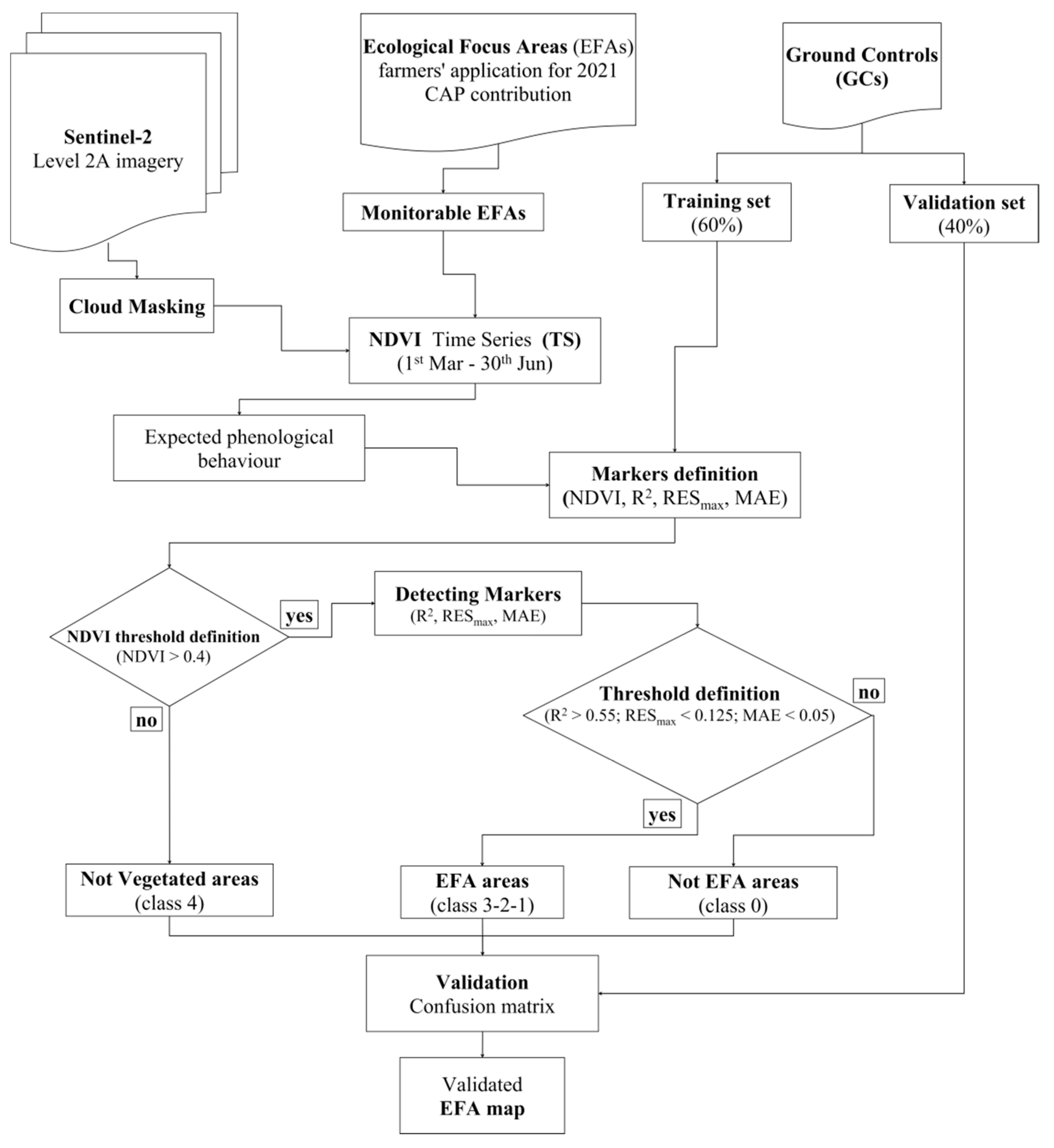
2.3.1. Composing NDVI Time Series

As previously mentioned, NDVI is one of the most widely used vegetation spectral indices in agriculture [50] to include applications related to the detection of agronomic practices [51]. Consequently, in this work, an approach based on the analysis of NDVI time series (TS) appeared to be suitable for detecting unauthorised practices within EFAs. TS was generated through a self-developed routine implemented in IDL v 8.0.1. [52], accounting for the following operational steps at pixel level: (a) local NDVI temporal profile extraction from TS; (b) removal of bad observations using SCL layer as driver; (c) profile smoothing by a symmetric Savitzky–Golay filter (kernel = 3, derivative = 0, degree = 1); and (d) profile regularization (time step = 5 days) by spline interpolation (tensor value = 10) [53,54]. It is worth noting that filtering, interpolation and regularization of NDVI profiles reduce the signal noise permitting highlighting of the most significant trend components over time [55]. Final TS resulted in a stack of 25 equally spaced NDVI time series maps covering RP.

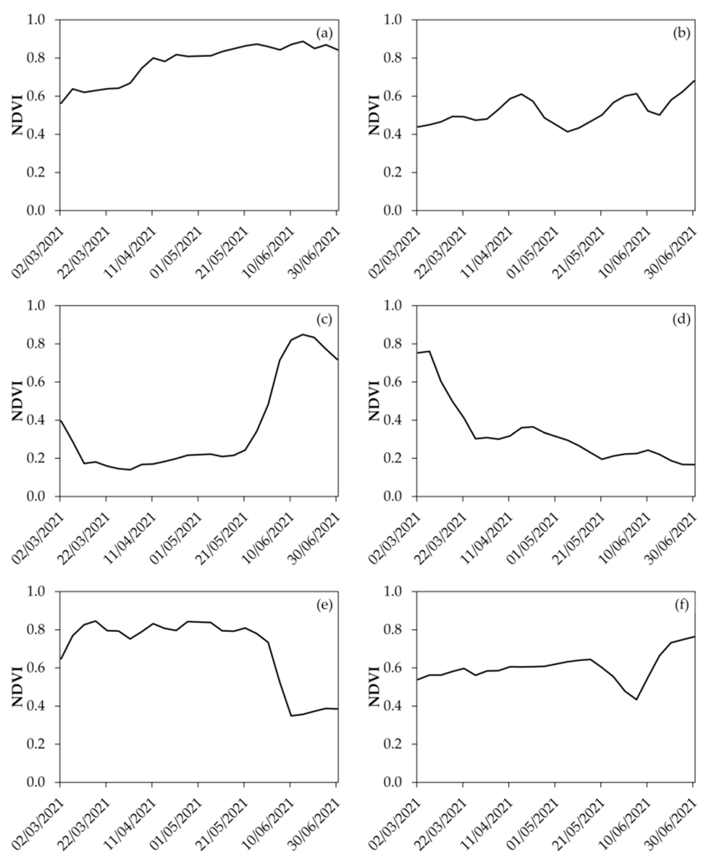
2.3.2. Looking for Markers within NDVI Temporal Profiles

Within EFAs, favourable conditions are expected to be present for the development of organisms and, consequently, of biodiversity. Intensive agriculture where no EFA is present can greatly compromise this natural mechanism by degrading the biologic value of large areas. EFAs are supported by CAP to ensure that farmers move their practices in the direction of better preserving the ecological value of agricultural environments. For this purpose, during spring, i.e. RP, farmers must stop all of their actions in the part of their fields that they declared as EFAs. Nevertheless, farmers often violate this restriction in an attempt to maximize the economical profit, which can increase if an additional field is cultivated. This makes it desirable for PPs to control farmers’ declarations concerning EFAs as widely as possible. NDVI TS can be used for this purpose, making it possible to detect (even retrospectively) the whole history of a farmer’s activities. These (mowing, sowing or harvesting) are generally associated with significant positive or negative variations alongside the local NDVI temporal profile [42]. Figure 3 shows some examples of the NDVI temporal profiles (field averaged) corresponding to six fields from GCs that farmers declared as EFAs. Some of them can be easily assigned to EFAs, while some others highlight evident variations, possibly related to the violation of CAP restrictions. In Figure 3a, the reported NDVI profile is the one expected for the natural development of vegetation related to an EFA. In Figure 3b, some significant variations in the profile can be recognized, possibly related to mowing operations. Figure 3c shows a profile that suggests sowing and the consequent growing of a crop. Figure 3d,f show profiles characterized by crop harvesting at the beginning and at the end of the growing period, respectively. Figure 3f shows a profile where a significant operation can be recognized in the middle of the controlled period. These examples cannot be assumed as general because the date and intensity of variations can vary enormously within an analysed period. Nevertheless, they are useful to demonstrate that some markers can be easily recognized alongside the NDVI temporal profiles to alert the possible presence of unexpected agronomic actions by which EFAs should not be affected.

2.3.3. Detecting Markers

Detection of markers was based on the analysis of the average TS profile of fields that were preventively computed by zonal statistics by SAGA GIS 7.9 [56].
Markers’ detection was achieved by composing a succession of rules that applied to the NDVI temporal profile of EFA-declared fields. The first condition we tested was that EFA-potential fields were vegetated during RP. Consequently, all GSAA plots never exceeding 0.4 NDVI value during RP were coded (code = 4) and excluded from the successive processing steps. The 0.4 NDVI value was set as the threshold, according to the literature, which reports that lower values correspond to not significant vegetation cover [57,58].
Concerning the vegetated fields, their expected phenological behavior during RP is consistent with natural vegetation. This is expected to show a continuous increasing trend in RP [59,60]. Consequently, if any agronomic practice occurred, it would generate an anomalous variation of the trend, determining significant differences that would possibly be detectable by exploring the residuals values between a hypothesized and modeled trend function and the actual NDVI temporal profile.
According to this idea, the authors modeled the phenological trend (hereafter called y i ) of the i-th EFA field (field averaged) by a first-order linear regression. Processing was achieved by R software [61,62]. The corresponding residuals were therefore calculated and assessed by computing some statistics to inform about these anomalies. In particular, the maximum residual absolute value (RESmax), the coefficient of determination (R2, [63,64]) and the mean absolute error (MAE, [65]) were computed and mapped for each GSAA field [65]. The RESmax was assumed to correspond to the maximum residual absolute value resulting from the calibrated model.

2.3.4. From Residual Statistics to Markers

To transform residual-related statistics into markers for anomaly detection, the RESmax, MAE and R2 statistical distributions were analysed by Otsu’s method. This method [66] proved to be an effective technique [67,68] for objectively defining a data-driven threshold by analysing the frequency distribution of the variable of interest. Otsu’s method is a nonparametric and unsupervised method that maximizes both the separability and the internal similarity of two groups of values through the identification of a proper threshold value from the histogram.
Concerning the present work, Otsu’s method was applied to the statistical distributions of the RESmax, MAE and R2 from the training set, thus obtaining three threshold values ( T M A E , T R 2   , T R E S ) useful for recognition of EFA fields at different reliability levels. The following conditions were tested according to Equation (2):
{ M A E > T M A E i f   N o   E F A R 2 > T R 2 i f   Y e s   E F A R E S m a x > T R E S i f   N o   E F A
Depending on the number of conditions that the i-th GSAA plot successfully satisfied, five different EFA classes were mapped. Class meaning is reported in Table 2.
Classification was then validated with reference to the validation set VP (made of 102 GCs) by computing the correspondent confusion matrix at the fields level. The related Overall Accuracy (OA), User’s Accuracy (UA) and Producer’s Accuracy (PA) were derived according to Hay [69]. An EFA map was used, finally, to derive operational information for control purposes. In Figure 4, a scheme of the proposed workflow is shown.

3. Results and Discussions

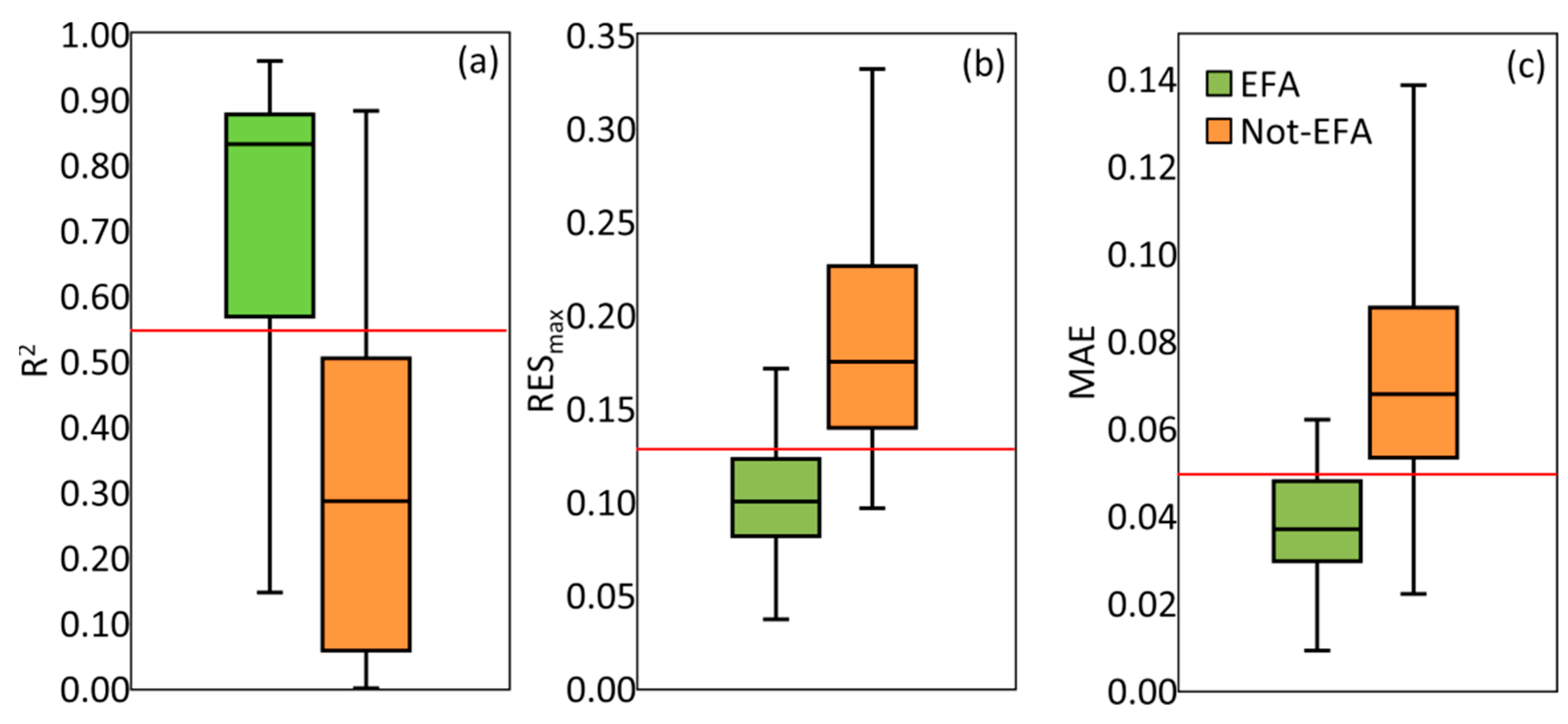
3.1. Threshold Definition

Once the NDVI trend was modeled at the field level, and residuals were computed, statistical distributions of the R2, RESmax and MAE from the TP dataset were analyzed for differences between EFA and non-EFA parcels. Figure 5 shows the thresholds found by Otsu’s method and boxplots summarizing the statistical distributions of the R2, RESmax and MAE. The obtained threshold values were 0.55; 0.125 and 0.05 for the R2, RESmax and MAE, respectively. The above-mentioned conditions were therefore tested at the field level for all EFA-declared plots in the area.
It is worth noting that threshold definition, based on Otsu’s method, was specifically aimed at avoiding subjective choices. The method is adaptive and data-driven, making it possible to automatically detect different threshold values according to the specific area one is considering. Consequently, the method can be applied wherever just by properly calibrating threshold values depending on the local agronomic conditions.

3.2. Classification and Validation

Classification was achieved by assigning each plot with the number of satisfied conditions (see Table 2). These were interpreted as classes of probability that the tested plot was actually an EFA. Classification was validated through computation of the correspondent confusion matrix (Table 3) obtained with reference to the VP dataset.
Table 3 shows that Classes 3, 0 and 4 are characterized by a very high UA: 77%, 91%, 100%, respectively. Conversely, Classes 2 and 1 show medium (57%) and low (4%) UA values, respectively. These situations make evident that the adoption of a single condition (Class 1), out of the three reported in Equation (2), is absolutely insufficient for the proper detection of EFA plots. This could be related to an intrinsic weakness of the modelled conditions or to causal elements, such as anomalies related to unfavourable climatic and environmental conditions within RP (frost, drought, precipitation or other natural interference) [70].
Concerning PA, the results were high for both the EFA (91%) and non-vegetated (100%) classes. Alternatively, results appear to be low (47%) for the non-EFA class. In fact, high confusion can be observed between Classes 0 and 1, where 23 non-EFA fields (35% out of the total) of VP were assigned to Class 1. This element further suggests that the satisfaction of a single condition, out of the tested three, is too weak for classification purposes. Consequently, one can admit that plots may be reasonably recognized as an EFA if at least two conditions are satisfied. With this new point of view in mind, the authors interpreted Classes 0 and 1 as related to non-EFA plots and Classes 2 and 3 as related to EFA plots at a different level of probability of detection. A new confusion matrix was therefore generated, and the correspondent UA and PA statistics were computed (Table 4).
After the new reorganisation of classes, more promising accuracy values were obtained. Specifically, the UA and PA of the non-EFA Classes 0 and 1 improved significantly, together with an OA that grew from 63% to 84%. These values are consistent with references from the literature. Zheng [71], using Landsat data for detecting changes in agricultural areas (Indiana, US), related agronomical practices through a multi-temporal analysis of vegetation indices (VIs) time series and found an OA of 90%. Dusseux [72] found that it was possible to detect agricultural practices (e.g. mowing of meadows) by satellite-derived VIs time series from SPOT (Satellite Pour l’Observation de la Terre) data in Brittany with an OA between 80 and 90%.

3.3. Interpreting EFA Map

In order to highlight the operational potentialities of an EFA map (Figure 6) with the above-mentioned accuracies, some quantitative information were obtained and discussed in light of CAP controls. In particular, area computation was achieved for the mapped classes and possible interpretations of the resulting percentages were given. Results are reported in Table 5.
Table 5 shows that, in the AOI, 6064 fields (about 48%) were classified as non-EFA, 378 (about 3%) were classified as non-vegetated and only 6068 (about 49% out of the total) were actually confirmed as an EFA (Classes 3 and 2). Specifically, for fields classified as an EFA, 3786 are in Class 3 (about 30%), and 2282 are in Class 2 (about 18%). Similar percentage values can be obtained with reference to their areas, in place of the number of fields.
To give an interpretation useful for CAP controls, it is worth noting that classified plots were only those that farmers declared as an EFA for the CAP campaign in 2021.
The first issue to be discussed is that the PA from classification in the control framework plays the most important role: to ensure the capability of the procedure to confirm or reject the hypothesis that the tested plot is actually an EFA.
Given the following conditions: (i) Classes 0-1 and Class 4 show a PA of 82 % and 100%, respectively; (ii) in the EFA map, about the 51% of controlled plots fall in these classes, therefore one can deduce that, with a probability of something more than 0.82, 51% of controlled 2021 EFA fields correspond to untruthful declarations from farmers. Consequently, Classes 0-1 and 4 as mapped in the EFA map require a field control. On the contrary, being that the PA of Class 3 is equal to 88%, we can reasonably admit that no controls are required for this class from PP, and the farmers’ declarations can be assumed compliant. For the 2021 campaign, class 3 corresponds to about 30% of controlled parcels that can avoid control by ground surveys.
To interpret the operational meaning of Class 2 for which no PA can be separately calculated, we can refer to the correspondent UA (57%). The UA defines the probability that only 57% of the Class 2 fields (about 18% of the total) are actually EFAs. This suggests that controls from PP are desirable in such a measure as they are obtainable via weighting programmed controls by this value. These preliminary results appear critical in terms of ordinary CAP controls strategy, highlighting a significant amount of possibly untruthful declarations detected with reasonably high accuracy via satellite data. These findings, obviously, raise intriguing questions regarding the CAP criteria for monitoring EFAs in order to ensure the properness of given economical grants. From this point of view, it is worth noting that ordinarily the ARPEA controls 5% of the received GSAA. A satellite-based approach, such as the one here presented, would guarantee a complete overview and the possibility of better focusing the GCs. Since controls are currently completely based on GCs, they cannot supply timely continuous information, which limits the controls to selected fields with a time that may not be exactly proper for the correct detection of the field management. Moreover, the time of the controls is strictly dependent on administrative constraints and, therefore, highly compromised in terms of synchronization with crop phenology. Depending on the time of the GC, some practices can be easily identified, such as the presence of other crops (i.e. corn, wheat), ploughing or harvesting. Others, however, such as mowing, may be almost impossible to detect if run too many days after the practice. These objective weaknesses of the current control process can be overcome by the utilization of satellite data, as demonstrated in this work.

4. Conclusions

In this work, a prototype service aimed at supporting PPs controls within the greening CAP framework, with special concern about Ecological Focus Area (EFA), is presented. Since the recent Italian National Report No. 5465 stipulates that mowing and any other soil management operations are prohibited on set-aside land designated as an EFA during RP, controls are required to test the respect for these conditions. The work was stimulated by the ARPEA for facing the operational task of EFA controls.
Since the ARPEA explicitly required that the classification approach was simple and explicit in its agronomical meaning, machine/deep learning-based (MDL) approaches were excluded. Conversely, a simpler, rule-based approach was developed for EFA detection based on the application of simple rules, or tasks, to disaggregate a complex problem into a succession of simple and more controllable ones, where agronomic knowledge plays a crucial role.
The method relies on the analysis of NDVI profiles from the Sentinel-2 mission, which is used for extracting three local statistics useful for EFA detection: the R2, RESmax and MAE. They were computed by approximating the local NDVI temporal profile in the reference period with a first-order polynomial. The EFA fields were recognized by testing the satisfaction of three threshold-based conditions. The threshold values were defined according to Otsu’s method and applied to a statistical distribution of the R2, RESmax and MAE from GCs. The correspondent 2021 EFA map was generated and validated.
The methodology was applied to a study area that included the administrative provinces of Torino, Asti and Vercelli (Piemonte Region, NW Italy). Specifically, over 12,510 EFA fields (CAP campaign 2021) were assessed to test the truthfulness of farmers’ GSAA declarations. Results showed an overall accuracy of 84%, indicating that the approach is promising. The authors retain that this procedure represents a valid alternative (or integrating) tool for ground controls by PPs. These preliminary results appear to be operationally critical in terms of CAP controls, highlighting a significant amount of possibly untruthful declarations detected with reasonably high accuracy via satellite data. These findings, obviously, raise intriguing questions regarding the present CAP criteria for monitoring EFAs in order to ensure the properness of given economical grants.
The procedure can be assumed applicable in every territory within the EU because EFAs do not depend on local crop types and behave similarly to natural meadows.
The procedure simply needs to be fine-tuned depending on the local agronomic calendar. In Italy, the reference period for testing conditions occurs between 1st March and 30th June (No. 5465, applying EU Regulation No. 1307/2013 of the European Parliament and Council).
Some limitations, however, still persist concerning the proposed procedure. One is possibly related to the presence of clouds over the AOI. In fact, the reference period useful for controls corresponds to the cloudiest period of th year. In unfavourable years, it is possible that detection will fail, since it relies entirely on optical data. Consequently, future development of the methodology could include a possible integration of SAR data from the S1 mission, as well as investigation into new phenological markers able to improve classification accuracy.

Author Contributions

Conceptualization, F.S.; methodology, F.S., S.D.P. and E.B.-M.; software, F.S. and S.D.P.; validation, F.S.; formal analysis, F.S. and S.D.P.; investigation, F.S. and E.B.-M.; resources, F.S.; data curation, F.S.; writing—original draft preparation, F.S., S.D.P. and E.B.-M.; writing—review and editing, F.S., S.D.P. and E.B.-M.; visualization, F.S., S.D.P. and E.B.-M.; supervision, E.B.-M. All authors have read and agreed to the published version of the manuscript.

Funding

This research received no external funding.

Informed Consent Statement

Informed consent was obtained from all subjects involved in the study.

Data Availability Statement

The data presented in this study are available on request from the corresponding author.

Acknowledgments

We would like to thank Elena Xausa and Gianluca Cantamessa, technicians for the Piemonte Regional Agency for Payments in Agriculture (ARPEA) for providing guidelines and fundamental operational information useful for reaching the results presented in this work.

Conflicts of Interest

The authors declare no conflict of interest.

References

  1. Ackrill, R. Common Agricultural Policy; A&C Black: London, UK, 2000; Volume 9. [Google Scholar]
  2. Grant, W. The Common Agricultural Policy; Macmillan International Higher Education: London, UK, 1997. [Google Scholar]
  3. Dupraz, P.; Guyomard, H. Environment and Climate in the Common Agricultural Policy. EuroChoices 2019, 18, 18–25. [Google Scholar] [CrossRef] [Green Version]
  4. Gowdy, J.M. The Value of Biodiversity: Markets, Society, and Ecosystems. Land Econ. 1997, 73, 25–41. [Google Scholar] [CrossRef]
  5. Lowe, P.; Feindt, P.H.; Vihinen, H. Introduction: Greening the Countryside? Changing Frameworks of EU Agricultural Policy. Public Adm. 2010, 88, 287–295. [Google Scholar] [CrossRef] [PubMed]
  6. Westhoek, H.; Van Zeijts, H.; Witmer, M.; Van den Berg, M.; Overmars, K.; Van der Esch, S.; Van der Bilt, W. Greening the CAP. An Analysis of the Effects of the European Commission’s Proposals for the Common Agricultural Policy 2014–2020; PBL Netherlands Environmental Assessment Agency: The Hague, The Netherlands, 2012. [Google Scholar]
  7. Gocht, A.; Ciaian, P.; Bielza, M.; Terres, J.-M.; Röder, N.; Himics, M.; Salputra, G. EU-Wide Economic and Environmental Impacts of CAP Greening with High Spatial and Farm-Type Detail. J. Agric. Econ. 2017, 68, 651–681. [Google Scholar] [CrossRef]
  8. Singh, M.; Marchis, A.; Capri, E. Greening, New Frontiers for Research and Employment in the Agro-Food Sector. Sci. Total Environ. 2014, 472, 437–443. [Google Scholar] [CrossRef]
  9. Wetzels, H. CAP Beyond the EU; Heinrich-Böll-Stiftung European Union: Ixelles, Belgium, 2021. [Google Scholar]
  10. Cagliero, R.; Licciardo, F.; Legnini, M. The Evaluation Framework in the New CAP 2023–2027: A Reflection in the Light of Lessons Learned from Rural Development. Sustainability 2021, 13, 5528. [Google Scholar] [CrossRef]
  11. Disposizioni Nazionali di Applicazione del Regolamento (UE) n. 1307/2013 del Parlamento Europeo e del Consiglio, del 17 Dicembre 2013; European Union: Brussels, Beglium, 2018.
  12. Regolamento Delegato (UE) n. 639/2014 della Commissione, dell’11 Marzo 2014, che Integra il Regolamento (UE) N. 1307/2013 del PARLAMENTO Europeo e del Consiglio Recante Norme sui Pagamenti Diretti Agli Agricoltori nell’Ambito dei Regimi di Sostegno Previsti dalla Politica Agricola Comune e che Modifica l’Allegato X di Tale Regolamento. 47; European Union: Brussels, Beglium, 2014.
  13. Zinngrebe, Y.; Pe’er, G.; Schueler, S.; Schmitt, J.; Schmidt, J.; Lakner, S. The EU’s Ecological Focus Areas—How Experts Explain Farmers’ Choices in Germany. Land Use Policy 2017, 65, 93–108. [Google Scholar] [CrossRef]
  14. Pe’Er, G.; Zinngrebe, Y.; Hauck, J.; Schindler, S.; Dittrich, A.; Zingg, S.; Tscharntke, T.; Oppermann, R.; Sutcliffe, L.M.; Sirami, C. Adding Some Green to the Greening: Improving the EU’s Ecological Focus Areas for Biodiversity and Farmers. Conserv. Lett. 2017, 10, 517–530. [Google Scholar] [CrossRef]
  15. Campinas, M.; Rosa, M.J. Assessing PAC Contribution to the NOM Fouling Control in PAC/UF Systems. Water Res. 2010, 44, 1636–1644. [Google Scholar] [CrossRef]
  16. Schiavon, E.; Taramelli, A.; Tornato, A.; Pierangeli, F. Monitoring Environmental and Climate Goals for European Agriculture: User Perspectives on the Optimization of the Copernicus Evolution Offer. J. Environ. Manag. 2021, 296, 113121. [Google Scholar] [CrossRef]
  17. Aschbacher, J. ESA’s Earth Observation Strategy and Copernicus. In Satellite Earth Observations and Their Impact on Society and Policy; Springer: Singapore, 2017; pp. 81–86. [Google Scholar]
  18. Bannari, A.; Morin, D.; Bonn, F.; Huete, A. A Review of Vegetation Indices. Remote Sens. Rev. 1995, 13, 95–120. [Google Scholar] [CrossRef]
  19. Leprieur, C.; Verstraete, M.M.; Pinty, B. Evaluation of the Performance of Various Vegetation Indices to Retrieve Vegetation Cover from AVHRR Data. Remote Sens. Rev. 1994, 10, 265–284. [Google Scholar] [CrossRef]
  20. Misra, G.; Cawkwell, F.; Wingler, A. Status of Phenological Research Using Sentinel-2 Data: A Review. Remote Sens. 2020, 12, 2760. [Google Scholar] [CrossRef]
  21. Boori, M.S.; Choudhary, K.; Paringer, R.; Sharma, A.K.; Kupriyanov, A.; Corgne, S. Monitoring Crop Phenology Using NDVI Time Series from Sentinel 2 Satellite Data. In Proceedings of the 2019 5th International Conference on Frontiers of Signal Processing (ICFSP), Marseille, France, 18–20 September 2019; pp. 62–66. [Google Scholar]
  22. Zhao, Y.; Potgieter, A.B.; Zhang, M.; Wu, B.; Hammer, G.L. Predicting Wheat Yield at the Field Scale by Combining High-Resolution Sentinel-2 Satellite Imagery and Crop Modelling. Remote Sens. 2020, 12, 1024. [Google Scholar] [CrossRef] [Green Version]
  23. Gómez, D.; Salvador, P.; Sanz, J.; Casanova, J.L. Potato Yield Prediction Using Machine Learning Techniques and Sentinel 2 Data. Remote Sens. 2019, 11, 1745. [Google Scholar] [CrossRef] [Green Version]
  24. Parida, B.R.; Kumar, A.; Ranjan, A.K. Crop Types Discrimination and Yield Prediction Using Sentinel-2 Data and AquaCrop Model in Hazaribagh District, Jharkhand. KN J. Cartogr. Geogr. Inf. 2021, 1–13. [Google Scholar] [CrossRef]
  25. Liu, R.; Huang, F.; Ren, Y.; Wang, P.; Zhang, J. Characterizing Ecosystem Functional Type Patterns Based on Subtractive Fuzzy Cluster Means Using Sentinel-2 Time-Series Data. J. Appl. Remote Sens. 2020, 14, 048505. [Google Scholar] [CrossRef]
  26. Andrew, M.E.; Wulder, M.A.; Nelson, T.A. Potential Contributions of Remote Sensing to Ecosystem Service Assessments. Prog. Phys. Geogr. 2014, 38, 328–353. [Google Scholar] [CrossRef] [Green Version]
  27. De Petris, S.; Sarvia, F.; Gullino, M.; Tarantino, E.; Borgogno-Mondino, E. Sentinel-1 Polarimetry to Map Apple Orchard Damage after a Storm. Remote Sens. 2021, 13, 1030. [Google Scholar] [CrossRef]
  28. Sarvia, F.; De Petris, S.; Borgogno Mondino, E. Multi-Scale Remote Sensing to Support Insurance Policies in Agriculture: From Mid-Term to Instantaneous Deductions. GISci. Remote Sens. 2020, 57, 770–784. [Google Scholar] [CrossRef]
  29. De Petris, S.; Sarvia, F.; Borgogno-Mondino, E. A New Index for Assessing Tree Vigour Decline Based on Sentinel-2 Multitemporal Data. Application to Tree Failure Risk Management. Remote Sens. Lett. 2021, 12, 58–67. [Google Scholar] [CrossRef]
  30. Momo, E.J.; De Petris, S.; Sarvia, F.; Borgogno-Mondino, E. Addressing Management Practices of Private Forests by Remote Sensing and Open Data: A Tentative Procedure. Remote Sens. Appl. Soc. Environ. 2021, 23, 100563. [Google Scholar] [CrossRef]
  31. Sarvia, F.; Petris, S.D.; Orusa, T.; Borgogno-Mondino, E. MAIA S2 Versus Sentinel 2: Spectral Issues and Their Effects in the Precision Farming Context. In Proceedings of the International Conference on Computational Science and Its Applications, Cagliari, Italy, 13–16 September 2021; pp. 63–77. [Google Scholar]
  32. Segarra, J.; Buchaillot, M.L.; Araus, J.L.; Kefauver, S.C. Remote Sensing for Precision Agriculture: Sentinel-2 Improved Features and Applications. Agronomy 2020, 10, 641. [Google Scholar] [CrossRef]
  33. Phiri, D.; Simwanda, M.; Salekin, S.; Nyirenda, V.R.; Murayama, Y.; Ranagalage, M. Sentinel-2 Data for Land Cover/Use Mapping: A Review. Remote Sens. 2020, 12, 2291. [Google Scholar] [CrossRef]
  34. Steinhausen, M.J.; Wagner, P.D.; Narasimhan, B.; Waske, B. Combining Sentinel-1 and Sentinel-2 Data for Improved Land Use and Land Cover Mapping of Monsoon Regions. Int. J. Appl. Earth Obs. Geoinf. 2018, 73, 595–604. [Google Scholar] [CrossRef]
  35. De Petris, S.; Boccardo, P.; Borgogno-Mondino, E. Detection and Characterization of Oil Palm Plantations through MODIS EVI Time Series. Int. J. Remote Sens. 2019, 40, 7297–7311. [Google Scholar] [CrossRef]
  36. Zheng, J.; Fu, H.; Li, W.; Wu, W.; Zhao, Y.; Dong, R.; Yu, L. Cross-Regional Oil Palm Tree Counting and Detection via a Multi-Level Attention Domain Adaptation Network. ISPRS J. Photogramm. Remote Sens. 2020, 167, 154–177. [Google Scholar] [CrossRef]
  37. Caballero, I.; Ruiz, J.; Navarro, G. Sentinel-2 Satellites Provide near-Real Time Evaluation of Catastrophic Floods in the West Mediterranean. Water 2019, 11, 2499. [Google Scholar] [CrossRef] [Green Version]
  38. De Petris, S.; Sarvia, F.; Borgogno Mondino, E. Multi-Temporal Mapping of Flood Damage to Crops Using Sentinel-1 Imagery: A Case Study of the Sesia River (October 2020). Remote Sens. Lett. 2021, 12, 459–469. [Google Scholar] [CrossRef]
  39. Campos-Taberner, M.; García-Haro, F.J.; Martínez, B.; Sánchez-Ruíz, S.; Gilabert, M.A. A Copernicus Sentinel-1 and Sentinel-2 Classification Framework for the 2020+ European Common Agricultural Policy: A Case Study in València (Spain). Agronomy 2019, 9, 556. [Google Scholar] [CrossRef] [Green Version]
  40. Sarvia, F.; Xausa, E.; Petris, S.D.; Cantamessa, G.; Borgogno-Mondino, E. A Possible Role of Copernicus Sentinel-2 Data to Support Common Agricultural Policy Controls in Agriculture. Agronomy 2021, 11, 110. [Google Scholar] [CrossRef]
  41. Kanjir, U.; \DJurić, N.; Veljanovski, T. Sentinel-2 Based Temporal Detection of Agricultural Land Use Anomalies in Support of Common Agricultural Policy Monitoring. ISPRS Int. J. Geo-Inf. 2018, 7, 405. [Google Scholar] [CrossRef] [Green Version]
  42. Bégué, A.; Arvor, D.; Bellon, B.; Betbeder, J.; De Abelleyra, D.; PD Ferraz, R.; Lebourgeois, V.; Lelong, C.; Simões, M.R.; Verón, S. Remote Sensing and Cropping Practices: A Review. Remote Sens. 2018, 10, 99. [Google Scholar] [CrossRef] [Green Version]
  43. Kaul, H.A.; Sopan, I. Land Use Land Cover Classification and Change Detection Using High Resolution Temporal Satellite Data. J. Environ. 2012, 1, 146–152. [Google Scholar]
  44. Kussul, N.; Lavreniuk, M.; Skakun, S.; Shelestov, A. Deep Learning Classification of Land Cover and Crop Types Using Remote Sensing Data. IEEE Geosci. Remote Sens. Lett. 2017, 14, 778–782. [Google Scholar] [CrossRef]
  45. Nguyen, T.T.; Hoang, T.D.; Pham, M.T.; Vu, T.T.; Nguyen, T.H.; Huynh, Q.-T.; Jo, J. Monitoring Agriculture Areas with Satellite Images and Deep Learning. Appl. Soft Comput. 2020, 95, 106565. [Google Scholar] [CrossRef]
  46. Gascon, F.; Cadau, E.; Colin, O.; Hoersch, B.; Isola, C.; Fernández, B.L.; Martimort, P. Copernicus Sentinel-2 Mission: Products, Algorithms and Cal/Val. In Earth Observing Systems XIX; International Society for Optics and Photonics: Bellingham, WA, USA, 2014; Volume 9218, p. 92181E. [Google Scholar]
  47. Delwart, S. SENTINEL-2 User Handbook. European Space Agency (ESA): Paris, France, 2015; Volume 1, pp. 1–64. [Google Scholar]
  48. Rouse, J.W.; Haas, R.H.; Schell, J.A.; Deering, D.W.; Harlan, J.C. Monitoring the Vernal Advancement and Retrogradation (Green Wave Effect) of Natural Vegetation; Technical Report No. E7410113; National Aeronautics and Space Administration: Washington, DC, USA, 1974. [Google Scholar]
  49. Richards, J.A.; Richards, J.A. Remote Sensing Digital Image Analysis; Springer: Berlin/Heidelberg, Germany, 1999; Volume 3. [Google Scholar]
  50. Shanmugapriya, P.; Rathika, S.; Ramesh, T.; Janaki, P. Applications of Remote Sensing in Agriculture-A Review. Int. J. Curr. Microbiol. Appl. Sci. 2019, 8, 2270–2283. [Google Scholar] [CrossRef]
  51. Veloso, A.; Mermoz, S.; Bouvet, A.; Le Toan, T.; Planells, M.; Dejoux, J.-F.; Ceschia, E. Understanding the Temporal Behavior of Crops Using Sentinel-1 and Sentinel-2-like Data for Agricultural Applications. Remote Sens. Environ. 2017, 199, 415–426. [Google Scholar] [CrossRef]
  52. Chen, J.; Jönsson, P.; Tamura, M.; Gu, Z.; Matsushita, B.; Eklundh, L. A Simple Method for Reconstructing a High-Quality NDVI Time-Series Data Set Based on the Savitzky–Golay Filter. Remote Sens. Environ. 2004, 91, 332–344. [Google Scholar] [CrossRef]
  53. Mishra, A.; Lu, Y.; Meng, J.; Anderson, A.W.; Ding, Z. Unified Framework for Anisotropic Interpolation and Smoothing of Diffusion Tensor Images. NeuroImage 2006, 31, 1525–1535. [Google Scholar] [CrossRef] [PubMed]
  54. Chen, Y.; Cao, R.; Chen, J.; Liu, L.; Matsushita, B. A Practical Approach to Reconstruct High-Quality Landsat NDVI Time-Series Data by Gap Filling and the Savitzky–Golay Filter. ISPRS J. Photogramm. Remote Sens. 2021, 180, 174–190. [Google Scholar] [CrossRef]
  55. Santos, L.A.; Ferreira, K.R.; Camara, G.; Picoli, M.C.; Simoes, R.E. Quality Control and Class Noise Reduction of Satellite Image Time Series. ISPRS J. Photogramm. Remote Sens. 2021, 177, 75–88. [Google Scholar] [CrossRef]
  56. Conrad, O.; Bechtel, B.; Bock, M.; Dietrich, H.; Fischer, E.; Gerlitz, L.; Wehberg, J.; Wichmann, V.; Böhner, J. System for Automated Geoscientific Analyses (SAGA) v. 2.1. 4. Geosci. Model Dev. 2015, 8, 1991–2007. [Google Scholar] [CrossRef] [Green Version]
  57. Gianinetto, M.; Rusmini, M.; Candiani, G.; Via, G.D.; Frassy, F.; Maianti, P.; Marchesi, A.; Nodari, F.R.; Dini, L. Hierarchical Classification of Complex Landscape with VHR Pan-Sharpened Satellite Data and OBIA Techniques. Eur. J. Remote Sens. 2014, 47, 229–250. [Google Scholar] [CrossRef] [Green Version]
  58. Borgogno-Mondino, E.; Lessio, A.; Gomarasca, M.A. A Fast Operative Method for NDVI Uncertainty Estimation and Its Role in Vegetation Analysis. Eur. J. Remote Sens. 2016, 49, 137–156. [Google Scholar] [CrossRef]
  59. Sarvia, F.; De Petris, S.; Borgogno-Mondino, E. Remotely Sensed Data to Support Insurance Strategies in Agriculture. In Remote Sensing for Agriculture, Ecosystems, and Hydrology XXI; International Society for Optics and Photonics: Bellingham, WA, USA, 2019; Volume 11149, p. 111491H. [Google Scholar]
  60. Hou, X.; Gao, S.; Niu, Z.; Xu, Z. Extracting Grassland Vegetation Phenology in North China Based on Cumulative SPOT-VEGETATION NDVI Data. Int. J. Remote Sens. 2014, 35, 3316–3330. [Google Scholar] [CrossRef]
  61. Verzani, J. Getting Started with RStudio; O’Reilly Media, Inc.: Newton, MA, USA, 2011. [Google Scholar]
  62. Gandrud, C. Reproducible Research with R and RStudio; Chapman and Hall/CRC: Boca Raton, FL, USA, 2018. [Google Scholar]
  63. Ozer, D.J. Correlation and the Coefficient of Determination. Psychol. Bull. 1985, 97, 307. [Google Scholar] [CrossRef]
  64. Di Bucchianico, A. Coefficient of Determination (R 2). Encycl. Stat. Qual. Reliab. 2008, 1. [Google Scholar]
  65. Willmott, C.J.; Matsuura, K. Advantages of the Mean Absolute Error (MAE) over the Root Mean Square Error (RMSE) in Assessing Average Model Performance. Clim. Res. 2005, 30, 79–82. [Google Scholar] [CrossRef]
  66. Otsu, N. A Threshold Selection Method from Gray-Level Histograms. IEEE Trans. Syst. Man Cybern. 1979, 9, 62–66. [Google Scholar] [CrossRef] [Green Version]
  67. Kurita, T.; Otsu, N.; Abdelmalek, N. Maximum Likelihood Thresholding Based on Population Mixture Models. Pattern Recognit. 1992, 25, 1231–1240. [Google Scholar] [CrossRef]
  68. Trier, O.D.; Jain, A.K. Goal-Directed Evaluation of Binarization Methods. IEEE Trans. Pattern Anal. Mach. Intell. 1995, 17, 1191–1201. [Google Scholar] [CrossRef]
  69. Hay, A.M. The Derivation of Global Estimates from a Confusion Matrix. Int. J. Remote Sens. 1988, 9, 1395–1398. [Google Scholar] [CrossRef]
  70. Wang, R.; Cherkauer, K.; Bowling, L. Corn Response to Climate Stress Detected with Satellite-Based NDVI Time Series. Remote Sens. 2016, 8, 269. [Google Scholar] [CrossRef] [Green Version]
  71. Zheng, B.; Campbell, J.B.; de Beurs, K.M. Remote Sensing of Crop Residue Cover Using Multi-Temporal Landsat Imagery. Remote Sens. Environ. 2012, 117, 177–183. [Google Scholar] [CrossRef]
  72. Dusseux, P.; Gong, X.; Hubert-Moy, L.; Corpetti, T. Identification of Grassland Management Practices from Leaf Area Index Time Series. J. Appl. Remote Sens. 2014, 8, 083559. [Google Scholar] [CrossRef]
Figure 1. The study area (green) is located in the Piemonte Region of NW Italy and corresponds to the administrative provinces of Torino, Asti and, partially, Vercelli. (Reference system is WGS84/UTM 32N, EPSG: 32632).
Agronomy 12 00406 g001
Figure 2. (a) Spatial distribution of the GCs used in the training and validation phase; (b) Spatial distribution of the GCs class type. (Reference system is WGS84/UTM 32N, EPSG: 32632).
Agronomy 12 00406 g002
Figure 3. NDVI temporal profiles (field averaged) for: (a) Ecological Forest Area profiles; (b) mowed meadow profile; (c) profile related to sowing and crop development; (d) profile showing a possible harvesting at the beginning of the controlled period; (e) profile showing a possible harvesting at the end of the period; and (f) profile showing a significant agronomic operation in the middle of the controlled period.
Agronomy 12 00406 g003
Figure 4. Workflow of the proposed methodology used for mapping and validating EFAs within the CAP controls framework. Wavy polygons stand for data input, rectangles for workflow operations and rhombuses are the binary decision nodes.
Agronomy 12 00406 g004
Figure 5. Boxplots of the R2, RESmax and MAE distributions for EFA and non-EFA: Black lines define (bottom-up) the 5th, 25th, 50th, 75th, and 95th percentiles; (a) R2 distribution; (b) MAXres distribution; (c) MAE distribution. Red lines indicate the threshold values defined by Otsu’s method and used in this work for each marker.
Agronomy 12 00406 g005
Figure 6. EFA map. (Reference system is WGS84/UTM 32N, EPSG: 32632).
Agronomy 12 00406 g006
Table 1. Number and size of surveyed fields carried out by the ARPEA per class type and relative split of the GCs involved in TP and VP.
ClassTotal Number of Surveyed FieldsTotal Area of Surveyed Fields (ha)Training Set (n. Fields)Training Set (ha)Validation Set (n. Fields)Validation Set (ha)
EFA95110.3557 (60%)64.7 (58%)38 (40%)46.2 (42%)
Non-EFA145191.8287 (60%)100.5 (52%)58 (40%)91.3 (48%)
Non-Vegetated 1516.189 (60%)10.1 (62%)6 (40%)6.1 (38%)
Table 2. Class code meaning according to the number of satisfied conditions set by Equation (2).
Class CodeN. of Satisfied ConditionsMeaning
33EFA plots (maximum probability)
22EFA plots (average probability)
11EFA plots (low probability)
00Non-EFA plots
4N/ANon-vegetated areas (non-EFA)
Table 3. Confusion matrix computed for the EFA map with reference to the VP dataset. Matrix elements contain the number of fields satisfying local conditions. Green cells are those used to compute OA.
ClassesReferenceTotalUser Accuracy (UA)
EFANon-EFANon-Vegetated
Classification320602677%
28601457%
11230244%
033103491%
40044100%
Total32664102
Producer Accuracy (PA)91%47%100% Overall Accuracy (OA) 63%
Table 4. Confusion matrix of EFA map after merging Classes 0 and 1 (non-EFA plots): Matrix elements are reported in the number of fields. Orange cells represent the number of fields used to compute OA.
ClassesReferenceTotalUser Accuracy (UA)
EFANon-EFANon-Vegetated
Classification320602677%
28601457%
0–145405893%
40044100%
Total 32664102
Producer Accuracy (PA)88%82%100% Overall Accuracy (OA) 84%
Table 5. Number of plots and corresponding area of the classes mapped within the EFA map.
ClassCodeFieldsFields (%)Total Area (ha)Total Area (%)
EFA (3)3378630.26%1921.6729.63%
EFA (2)2228218.24%1083.9816.71%
Non-EFA 0–1606448.47%3205.4649.42%
Non-vegetated 43783.02%275.024.24%
Total-125101006486.13100
Publisher’s Note: MDPI stays neutral with regard to jurisdictional claims in published maps and institutional affiliations.

