Describing Lettuce Growth Using Morphological Features Combined with Nonlinear Models

Abstract

The aim of this study was to describe the sigmoidal growth behaviour of a lettuce canopy using three nonlinear models. Gompertz, Logistic and grey Verhulst growth models were established for the top projected canopy area (TPCA), top projected canopy perimeter (TPCP) and plant height (PH), which were measured by two machine vision views and 3D point clouds data. Satisfactory growth curve fitting was obtained using two evaluation criteria: the coefficient of determination (R²) and the mean absolute percentage error (MAPE). The grey Verhulst models produced a better fit for the growth of TPCA and TPCP, with higher R² ($R_{TPCA}^2=0.9097, R_{TPCP}^2=0.8536$) and lower MAPE ($MAP{E}_{TPCA}^{}=0.0284, MAP{E}_{TPCP}^{}=0.0794$) values, whereas the Logistic model produced a better fit for changes in PH ($R_{PH}^2=0.8991,MAP{E}_{PH}^{}=0.0344$). The maximum growth rate point and the beginning and end points of the rapid growth stage were determined by calculating the second and third derivatives of the models, permitting a more detailed description of their sigmoidal behaviour. The initial growth stage was 1–5.5 days, and the rapid growth stage lasted from 5.6 to 26.2 days. After 26.3 days, lettuce entered the senescent stage. These inflections and critical points can be used to gain a better understanding of the growth behaviour of lettuce, thereby helping researchers or agricultural extension agents to promote growth, determine the optimal harvest period and plan commercial production.

1. Introduction

Lettuce is widely cultivated throughout the world. It plays an important role in human nutrition and has, therefore, become a subject of research focus in recent years [1,2]. China is responsible for more than half of the world’s lettuce production. Lettuce has a short growth period and a high growth rate, and both its old and new leaves are edible vegetables [3]. Monitoring the growth of lettuce by accurately obtaining growth-related traits is of great practical significance for optimising management and maximising production [4]. The use of growth models and critical points can guide fertilisation and harvest [5].

Plant growth is a complex and highly dynamic process [6]. Growth models play an important role in the prediction of growth and yield, accurately predicting the size and growth rate of plants at different growth stages [7], determining the optimal harvest period and guiding economic decisions based on plant growth mechanisms. They permit the scientific and rational determinations of plant growth regulation patterns and the quantification of plant growth cycles and phenotypic characteristics at different growth stages [8]. Previous studies have shown that the growth of both internal cells and tissues and external roots, stems, leaves, seeds and fruits follows a “slow-fast-slow” pattern [9], which can be described by growth models [10]. In such models, the growth and growth rate in early stages are greater than those in later stages, producing a sigmoidal growth curve [11]. Nonlinear regression models are, therefore, important tools because many crop growth processes are better represented by nonlinear models than by linear models [12].

The Gompertz model [13], the Logistic model [14,15] and the grey Verhulst model [16,17] are curvilinear equations commonly used to describe growth processes and are widely applied to establish mathematical models of plant phenotypic characteristics [18,19]. For example, such models have been used to describe the growth of morphological traits in sunn hemp [20,21], cashew fruits [22], sunflowers [23], pears [24] and sudangrass [25]. However, nonlinear regression is still seldom used for statistical analysis in vegetable crop trials [26], and when it is used, it is rarely applied to growth models of production. Growth models have proven to be efficient statistical analysis tools. They have been used to predict production behaviour, which can be quantified by the models’ inflection and critical points. These points are extremely important in terms of growth behaviour and can be mathematically determined from growth curves [27]. Zhang et al. proposed a method for estimating growth-related traits of multiple cultivars of greenhouse lettuce using digital images and a convolutional neural network [4]. However, most previous manuscripts have only identified the model with the best goodness-of-fit and have ignored the growth points [28,29].

This study was conducted to establish the morphological features (MFs) of the sigmoidal growth models of the lettuce canopy based on two machine vision views and 3D point clouds data. The second and third derivatives of the models were calculated and used to identify the maximum growth rate points and rapid growth stages. This study provides a basis for variable rate fertilisation and timely harvest based on growth trends.

2. Materials and Methods

2.1. Plant Material

The experimental material was lettuce (Lactuca sativa L. Italian, Woshu Seeds Co. Ltd., Nanjing, China), and the experiment was performed in a greenhouse at Jiangsu University in China (32.11° N, 119.27° E). All plants were transplanted when they had five true leaves and were grown under non-soil conditions with three independent repeated experiments in the spring at one-week intervals from late April to early June 2020, yielding 54 samples. The nutrient solution was prepared according to the Yamasaki lettuce recipe, and its composition was: Ca(NO₃)₂·4H₂O, 236 mg·L⁻¹; KNO₃, 404 mg·L⁻¹; NH₄H₂PO₄, 57 mg·L⁻¹; MgSO₄·7H₂O, 123 mg·L⁻¹; Fe–EDTA, 16 mg·L⁻¹; MnCl₂·4H₂O, 1.2 mg·L⁻¹; H₃BO₃, 0.72 mg·L⁻¹; ZnSO₄·4H₂O, 0.09 mg·L⁻¹; CuSO₄·5H₂O, 0.04 mg·L⁻¹; and (NO₄)₂Mo₇O₄, 0.01 mg·L⁻¹. Each group of lettuce roots was maintained on a fixed concentration of nutrient solution using a self-developed, timed irrigation and collection system [30]. Pest and disease management followed the technical recommendations for the crop. Climate data were collected by multiple sensors situated in the greenhouse. The night temperature was not lower than 15 °C, the day temperature was not higher than 30 °C, and the light intensity was 200–400 µmol·m⁻²·s⁻¹.

2.2. Computer Vision Data Acquisition

Two strategies were used to describe the lettuce canopy growth. Images of the lettuce canopy were obtained using two digital cameras placed in a custom-made optical box. One of the cameras was positioned above the top of the canopy to obtain top view images, and another camera was positioned at the front of the canopy to obtain front view images. A white background plate was fixed to the lettuce roots, and normal graph paper was placed in the images. To ensure that the optical box was completely sealed, the images were collected by time-lapse photography with the aperture priority mode selected. The camera aperture was set to f/8, and ISO was set to 100. The colorific equipoise of the images could be controlled in the automatic exposure mode during the time of exposure; therefore, the colour images acquired were true red, green and blue bands. The images were stored in high-definition JPEG format with a resolution of 3888 × 2592.

2.3. 3D Point Clouds Data Collection

The point clouds data of the lettuce canopy in this study were obtained with a light-field camera (R26; Raytrix GmbH, http://www.raytrix.de/ accessed on 28 March 2022) and a high-speed GPU (NVIDIA RTX 2080). The imaging lens was a 3D light-field lens with a focal length of 100 mm and an aperture of f/2.80. Two light sources with adjustable brightness were installed at both sides of the light-field camera. Prior to the first scan, the microlens array calibration and metric calibration were performed. The resolution of the light-field camera was 7000 × 6000.

2.4. Nonlinear Growth Models

Three different nonlinear regression models (Gompertz, Logistic and grey Verhulst) were fitted and compared in our statistical analysis. The expressions of the first two growth curve models were as follows:

$$GompertzmodelY=K{m}^n{}^{{}^t}$$

(1)

$$LogisticmodelY=\frac{L}{1+c{e}^{-rt}}$$

(2)

where Y denotes the t^th observation; K, m, n, L, c and r denote estimated from the data; and t denote number of observations.

The variation rule of the grey Verhulst model is consistent with the settlement curve in the entire process. It has a characteristic sigmoidal type, which is similar to Gompertz and logistic growth models. The equation of the grey Verhulst model is as follows [16]:

$${{\displaystyle \widehat{x}}}^{(1)}(t+1)=\frac{a{x}_{}^{(0)}(1)}{b{x}_{}^{(0)}(1)+(a-b{x}_{}^{(0)}(1){)\mathrm{e}}^{at}}$$

(3)

where ${{\displaystyle \widehat{x}}}^{(1)}(t+1)$ denotes the prognostic value sequence; ${{\displaystyle x}}^{(0)}(1)$ denotes the initial measured value, ${{\displaystyle x}}^{(0)}(1)={{\displaystyle \widehat{x}}}^{(1)}(1)$; and a and b denote the development coefficient and grey action estimated from the data.

We used two comparison criteria to test the goodness-of-fit of the growth regression models—the coefficient of determination (R²) [13] and the mean absolute percentage error (MAPE) [31]:

$$R^2=1-\frac{{\displaystyle \sum _{i=1}^n{{\displaystyle (y_t-{\widehat{y}}_t)}}^2}}{{\displaystyle \sum _{i=1}^n{{\displaystyle (y_t-\overline{y})}}^2}}$$

(4)

$$MAPE=\frac{1}{n}{\displaystyle \sum _{i=1}^n\left|\left.\frac{y_t-{\widehat{y}}_t}{y_t}\right|\right.}\times 100\%$$

(5)

where $y_{\mathrm{i}}$ denotes the observed value, ${\widehat{y}}_i$ denotes the predicted value, n denotes the number of observations, and $\overline{y}$ denotes the mean value of the observations.

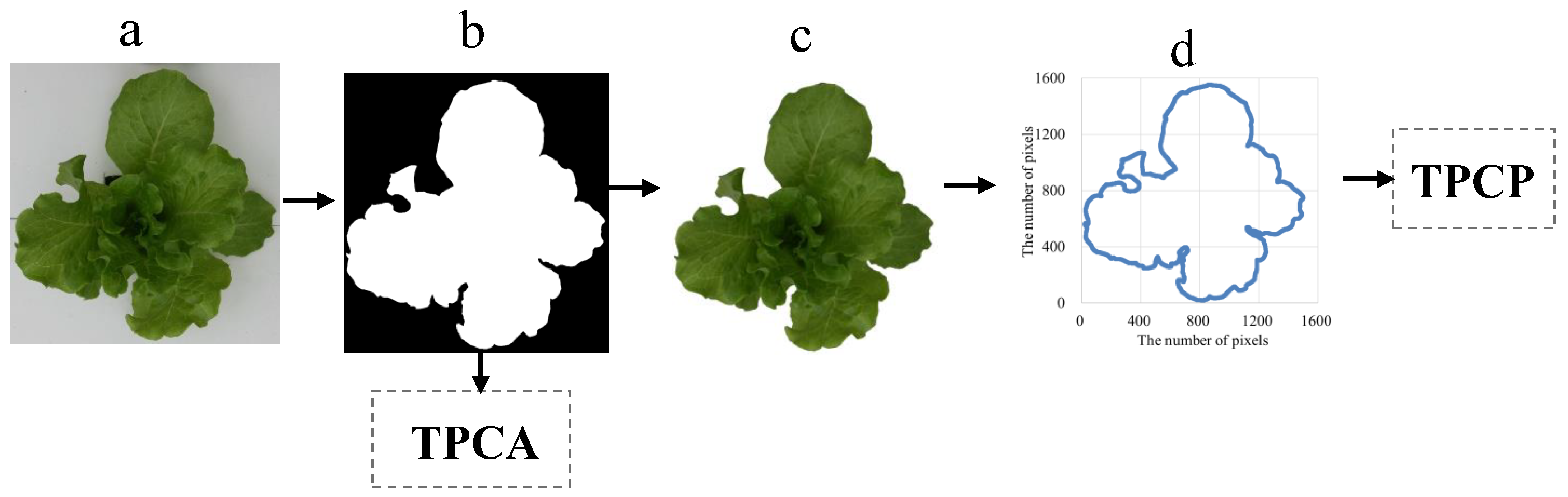
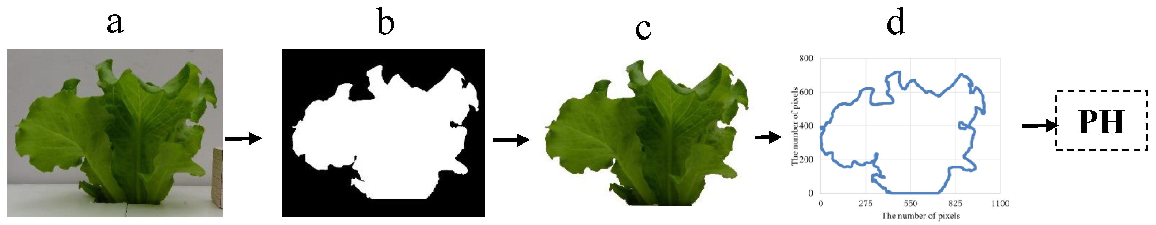
2.5. Extraction of Lettuce Canopy MFs from RGB Images

Three MFs were selected to reflect the nutritional status, growth and yield of lettuce from 3D point clouds data: top projected canopy area (TPCA), top projected canopy perimeter (TPCP) and plant height (PH) [32,33,34]. Figure 1 and Figure 2 illustrate the sequence of binarization, background segmentation, edge extraction and feature extraction. The binary images (Figure 1b and Figure 2b) were extracted using a threshold determined by the experimentation and the application of the “2G-R-B” index (Figure 1a and Figure 2a). Then, the TPCA of each plant was obtained by dividing the number of white pixels by a previously determined conversion factor. Background segmentation images are shown in Figure 1c and Figure 2c. Next, the Roberts, Sobel, Laplacian, Gaussian, Canny and zero-cross edge detector algorithms [35] were applied to extract TPCP and PH. Comparisons showed that the Canny edge detector was particularly suitable for these images; edges detected by this method not only contained fewer pixels but also had good closeness and true edges. The images were placed in rectangular coordinates (Figure 1d and Figure 2d).

TPCA, TPCP and PH were calculated according to the following equations:

$$TPCA=\frac{N_L}{f_1}$$

(6)

$$TPCP=\frac{N_P}{\sqrt{f_1}}$$

(7)

$$PH=\frac{N_H}{f_2}$$

(8)

where N_L denotes the total number of pixels in the lettuce area, f₁ denotes the number of pixels per unit area (1 cm²) in the top view images, N_P denotes the total number of pixels on the outer edge, N_H denotes the total number of pixels in the height direction, and f₂ denotes the number of pixels per centimetre in the front view images.

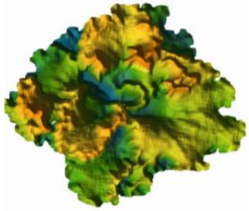
2.6. Extraction of Lettuce Canopy MFs from 3D Point Clouds Data

In this work, the bilateral filter was used to eliminate noise, which was generated due to device accuracy, environmental factors and operator experience [36]. The voxel-based grid method was used to reduce the large amount of redundant data because the light-field camera captures very detailed features of lettuce. As shown in Figure 3, the number of point cloud points was reduced from 849,234 (Figure 3a) to 19,346 (Figure 3b); the accuracies of TPCA, TPCP and PH were still more than 99%. The convex hull algorithms in rapid was used to calculate the TPCA and TPCP (Figure 4). As shown in Figure 5, the height of the lettuce canopy was represented by different colours, and PH was defined as the maximum.

3. Results

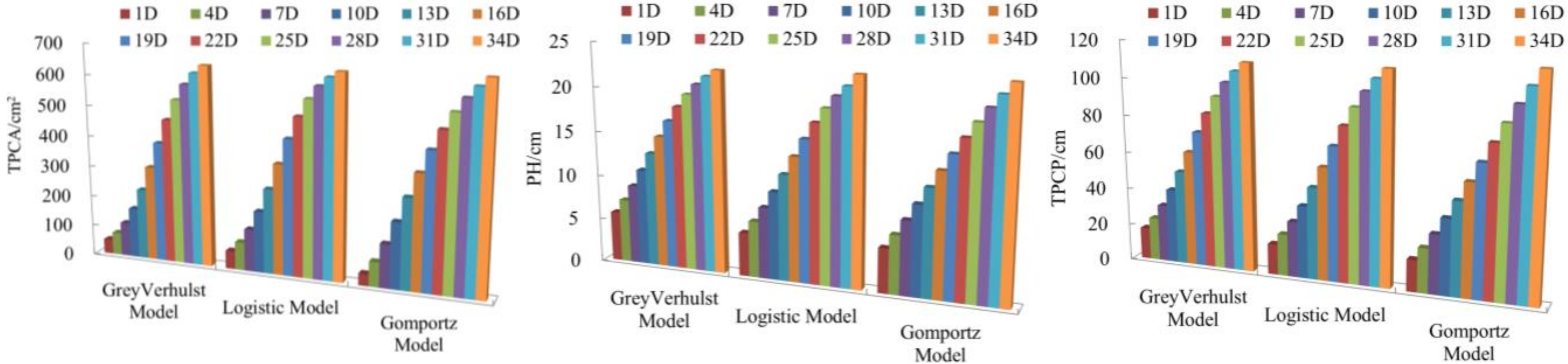
3.1. Establishment of Gompertz, Logistic and Grey Verhulst prediction Models

Three MFs measurements were taken for each sample in order to attain a reduction in error by averaging computer vision data and 3D point clouds data. The growth and growth rate of TPCA, PH and TPCP were greater in the early growth stage than in the later stage, producing a sigmoidal curve. This figure illustrates that the curves are appropriate for fitting the Gompertz, Logistic and grey Verhulst models. The equations of the Gompertz and Logistic models fitted to the three MFs are shown in

Table 1. The Gompertz and Logistic prediction models for TPCA, PH and TPCP.

MFs	Gompertz Model		Logistic Model
TPCA	$Y=751.6232\times {0.0192}^{0.751}{}^{{}^t}$	(9)	$Y=\frac{683.9952}{1+17.3906\times e^{-0.4909t}}$	(12)
PH	$Y=32.1068\times {0.1125}^{0.8538}{}^{{}^t}$	(10)	$Y=\frac{25.1288}{1+5.7471\times e^{-0.3265t}}$	(13)
TPCP	$Y=184.0483\times {0.063}^{0.8608}{}^{{}^t}$	(11)	$Y=\frac{126.2673}{1+9.5771\times e^{-0.3617t}}$	(14)

, and those of the grey Verhulst models are shown in

Table 2. The grey Verhulst prediction models for TPCA, PH and TPCP.

MFs	a	b	Grey Verhulst Models
TPCA	−0.4777	−0.0006895	${\widehat{x}}^{(1)}(t+1)=\frac{22.555}{0.03256+0.4451{\mathrm{e}}^{-0.4777t}}$	(15)
PH	−0.3259	−0.1133	${\widehat{x}}^{(1)}(t+1)=\frac{1.8239}{0.0741+0.2519e^{-0.3259t}}$	(16)
TPCP	−0.3664	−0.002972	${\widehat{x}}^{(1)}(t+1)=\frac{6.2434}{0.05063+0.3159e^{-0.3665t}}$	(17)

. The three predicted model curves are shown in Figure 6.

3.2. Model Selection

The fitting results of the three models are shown in

Table 3. Evaluation results for the TPCA, PH and TPCP growth models.

MFs	Comparison Criteria	Gompertz	Logistic	Grey Verhulst
TPCA	R2	0.8496	0.8746	0.9097
	MAPE	0.0841	0.0393	0.0284
PH	R2	0.8535	0.8991	0.8978
	MAPE	0.0472	0.0344	0.0349
TPCP	R2	0.8099	0.8272	0.8536
	MAPE	0.0919	0.0801	0.0794

. R² was an important and useful tool for comparing the growth models because of its high explanatory power. Table 3 shows that the R² values were higher than 0.80 for all models, indicating that the data generally fit well with the models that converged. However, the R² of TPCP was lower than those of TPCA and PH. The grey Verhulst model of TPCA and TPCP had higher R² and lower MAPE, which were superior to the Gompertz and Logistic models. Therefore, the grey Verhulst model best explained TPCA and TPCP growth, whereas the Logistic model best explained PH growth.

3.3. Determination of the Three Points

Three critical points were determined according to the methodology proposed by Mischan et al. [27]. In order to preferably compute the result, the Logistic growth model for PH ($Y=\frac{25.1288}{1+5.7471\times e^{-0.3265t}}$) was transformed into:

$$Y=\frac{25.1288}{1+e^{1.7487-0.3265t}};(Y=\frac{L}{1+e^{\alpha -\beta t}})$$

(18)

Then, $\alpha$ = 1.7487 and $\beta$ = 0.3265.

By calculating the second and third derivatives of the TPCA and TPCP grey Verhulst models and the PH Logistic model, we obtained formulas for the inflection points and the starting and ending points of the rapid growth stage, as shown in

Table 4. Formulas for inflection points and rapid growth stages.

MFs	Maximum Growth Rate Point *
TPCA	$t_{}^{*}=-3ln(\frac{a{b}^{-1}}{47.2145}-1)\cdot a^{-1}$	(19)
PH	$t_{}^{*}=\frac{3\alpha }{\beta }$	(20)
TPCP	$t_{}^{*}=-3ln(\frac{a{b}^{-1}}{17.0352}-1)\cdot a^{-1}$	(21)
MFs	Starting point of rapid growth stage
TPCA	$t_{}^{\mathrm{S}}=-3\left[ln(\frac{a{b}^{-1}}{47.2145}-1)-1.317\right]\cdot a^{-1}$	(22)
PH	$t_{}^{\mathrm{S}}=\frac{3(\alpha -1.317)}{\beta }$	(23)
TPCP	$t_{}^{\mathrm{S}}=-3\left[ln(\frac{a{b}^{-1}}{17.0352}-1)-1.317\right]\cdot a^{-1}$	(24)
MFs	Ending point of rapid growth stage
TPCA	$t_{}^{\mathrm{E}}=-3\left[ln(\frac{a{b}^{-1}}{47.2145}-1)+1.317\right]\cdot a^{-1}$	(25)
PH	$t_{}^{\mathrm{E}}=\frac{3(\alpha +1.317)}{\beta }$	(26)
TPCP	$t_{}^{\mathrm{E}}=-3\left[ln(\frac{a{b}^{-1}}{17.0352}-1)+1.317\right]\cdot a^{-1}$	(27)

* a and b values were obtained from Table 2.

. In the grey Verhulst model, ab⁻¹ was the upper limit value of the TPCA and TPCP theoretical growth, which were 692.8 cm² and 123.3 cm, respectively. In the Logistic model, L was the upper limit value of the PH theoretical growth, which was 25.1 cm.

In this study, three growth points were determined in lettuce, and the entire growth period was divided into three stages. In

Table 5. Inflection points and rapid growth stages.

MFs	Maximum Growth Rate Point (days)	Starting Point of Rapid Growth Stage (Days)	Ending Point of Rapid Growth Stage (Days)	Rapid Growth Stage (Days)
TPCA	16.4	8.2	24.7	16.5
PH	16.1	4.0	28.2	24.2
TPCP	18.0	4.2	25.8	21.6
Average	16.8	5.5	26.2	20.8

, the first growth point occurred at 16.8 days and indicated both the plant’s maximum growth rate and the time at which it occurred. The other two growth points were the starting and ending points of the rapid growth stage. The initial growth stage was 1-5.5 days, and the rapid growth stage lasted from 5.6 to 26.2 days. After 26.3 days, lettuce entered the senescent stage.

4. Discussion

4.1. Growth Models

The accurate monitoring of lettuce growth is critical for the optimised management of lettuce production. MFs are indicators to characterise the growth of lettuce [4]. Previous studies have shown that the Gompertz and Logistic nonlinear models are the most common methods in the description of the growth of plants’ MFs [5,10,23]. In this study, considering the two goodness-of-fit indicators (R² and MAPE), the grey Verhulst model had suitable behaviour and is the best indicated for describing the TPCA and TPCP of lettuce.

These results can be explained by the following reason. Due to the noise from both inside and outside the agriculture system, the information we can reach about that system is always uncertain and limited in scope. Hence, the agriculture system can be considered as a grey system [37]. Even a controllable greenhouse environment always contains some grey characteristics due to the time-varying parameters of the system [38]. For instance, the meteorological parameters (temperature, light intensity and humidity) are still uncertain factors. There was no significant difference between the R² and MAPE of the Logistic model and the grey Verhulst model for describing changes in PH.

4.2. Growth Points

Inflection points are used to infer crop growth, having as a base the general behaviour towards the cultivars [10]. In this study, the second and third derivatives were set to zero, and the maximum growth rate points and rapid growth stages were calculated, as shown in Table 5. Most previous manuscripts have only identified models with the best goodness-of-fit [28,39,40]. Lettuce exhibits high growth rates in controlled environments, and the differentiation among its growth stages is not clear-cut. It is, therefore, extremely important to determine the critical points in the lettuce growth curves compared to other plants [10]. As shown in Table 5, PH and TPCP entered rapid growth first and reached a maximum growth rate earlier than TPCA. This reflects the fact that leaf length growth is greater than leaf width growth in the early growth stage, whereas leaf length and width increase rapidly and simultaneously in later stages. In the later period, leaf differentiation was rapid, leaf density increased and the leaf ball was compact. Therefore, the end points of TPCA and TPCP were similar.

In addition, the critical points have been used in many studies in agricultural sciences as it provides relevant information on crop management [23]. Searching for the “maximum growth rate point” is important in crop research because it permits adjustments of nutritional inputs when the growth rate is at a maximum [27]. When it is reached, the curve changes in the concavity and the growth rate starts to decrease [5]. According to Lobo et al. and Valadão et al., fertiliser coverage applications would have optimised results if they were carried out in the rapid growth stage [41,42].

In this study, lettuce growth was slow in the initial growth stage. There is a rapid increase in nutritional demand in the rapid growth stage [18]; rational fertilisation would have optimised results in the senescent stage, and there were little changes in any of the MFs, which can be used as a maturity indicator. At this point, lettuce start growth stabilization and can be harvested. For lettuce, premature harvests result in low yields, whereas later harvests can cause poor taste. Therefore, the end point of the rapid growth stage and the upper limit value of theoretical growth are used to determine the age at which a vegetable crop reaches maturity [43,44]. They predict the best harvest time for an optimal yield and quality, thereby increasing the likelihood of early financial returns for farmers.

5. Conclusions

Nonlinear models can describe sigmoidal growth behaviour of the lettuce canopy mathematically based on two machine vision views and 3D point clouds data. Three growth models were used to fit the growth process of three morphological features of the lettuce canopy. The grey Verhulst model provided the best fit for the top projected canopy area and the top projected canopy perimeter with a higher R² and a lower mean absolute percentage error than the other models. The Logistic model was the best at describing changes in PH. The inflection and critical points were determined by calculating the second and third derivatives of the selected models. This study provides guidance for proper fertilisation timing in lettuce to promote growth and timely harvest. Although the proposed method has been shown to be accurate and efficient, there are still limitations that we need to take into account. Future studies will continue to collect more information to enlarge our dataset, such as biomass, leaves number, canopy volume and so on.

References

1. Zou, J.; Fanourakis, D.; Tsaniklidis, G.; Cheng, R.F.; Yang, Q.C.; Li, T. Lettuce growth, morphology and critical leaf trait responses to far-red light during cultivation are low fluence and obey the reciprocity law. Sci. Hortic. 2021, 289, 110455. [Google Scholar] [CrossRef]
2. Chen, Y.C.; Fanourakis, D.; Tsaniklidis, G.; Aliniaeifard, S.; Yang, Q.C.; Li, T. Low UVA intensity during cultivation improves the lettuce shelf-life, an effect that is not sustained at higher intensity. Postharvest Biol. Technol. 2021, 172, 11. [Google Scholar] [CrossRef]
3. Zhao, L.Q.; Zhang, Y.W.; Wang, L.; Liu, X.W.; Zhang, J.R.; He, Z.Y. Stereoselective metabolomic and lipidomic responses of lettuce (Lactuca sativa L.) exposing to chiral triazole fungicide tebuconazole. Food Chem. 2022, 371, 131209. [Google Scholar] [CrossRef] [PubMed]
4. Zhang, L.; Xu, Z.; Xu, D.; Ma, J.; Chen, Y.; Fu, Z. Growth monitoring of greenhouse lettuce based on a convolutional neural network. Hortic. Res 2020, 7, 124. [Google Scholar] [CrossRef] [PubMed]
5. Jane, S.A.; Fernandes, F.A.; Silva, E.M.; Muniz, J.A.; Fernandes, T.J.; Pimentel, G.V. Adjusting the growth curve of sugarcane varieties using nonlinear models. Cienc. Rural 2020, 50, e20190408. [Google Scholar] [CrossRef]
6. White, A.C.; Rogers, A.; Rees, M.; Osborne, C.P. How can we make plants grow faster? A source-sink perspective on growth rate. JExB 2016, 67, 31–45. [Google Scholar] [CrossRef]
7. Jiao, X.; Zhang, H.C.; Zheng, J.Q.; Yin, Y.; Wang, G.S.; Chen, Y.; Yu, J.; Ge, Y.F. Comparative analysis of nonlinear growth curve models for Arabidopsis thaliana rosette leaves. Acta Physiol. Plant. 2018, 40, 114. [Google Scholar] [CrossRef]
8. Ofir, M.; Kigel, J. Variation in onset of summer dormancy and flowering capacity along an aridity gradient in Poa bulbosa L., a geophytic perennial grass. Ann. Bot. 2003, 91, 391–400. [Google Scholar] [CrossRef] [Green Version]
9. Kumar, A.; Yadav, R.; Gupta, S.; Gaikwad, K.B.; Jain, N.; Ranjan, R.; Kumar, M. Identification of genotypes and marker validation for grain filling rate and grain filling duration in wheat under conservation agriculture. Indian J. Genet. Plant Breed. 2018, 78, 309–316. [Google Scholar]
10. Carini, F.; Cargneltitti, A.; Pezzini, R.V.; de Souza, J.M.; Chaves, G.G.; Procedi, A. Nonlinear models for describing lettuce growth in autumn-winter. Cienc. Rural 2020, 50, 12. [Google Scholar] [CrossRef]
11. Birch, C.P.D. A New Generalized Logistic Sigmoid Growth Equation Compared with the Richards Growth Equation. Ann. Bot. 1999, 83, 713–723. [Google Scholar] [CrossRef] [Green Version]
12. Archontoulis, S.V.; Miguez, F.E. Nonlinear Regression Models and Applications in Agricultural Research. Agron. J. 2015, 107, 786–798. [Google Scholar] [CrossRef] [Green Version]
13. Karadavut, U.; Palta, C.; Kokten, K.; Bakoglu, A. Comparative Study on Some Non-linear Growth Models Describing Leaf Growth of Maize. Int. J. Agric. Biol. 2010, 12, 227–230. [Google Scholar]
14. Tsoularis, A.; Wallace, J. Analysis of logistic growth models. Math. Biosci. 2002, 179, 21–55. [Google Scholar] [CrossRef] [Green Version]
15. Veloso, R.C.; Winkelstroter, L.K.; Silva, M.T.P.; Pires, A.V.; Torres, R.A.; Pinheiro, S.R.F.; Costa, L.S.; Amaral, J.M. Selection and classification of multivariate nonlinear models for broilers. Arq. Bras. Med. Vet. Zootec. 2016, 68, 191–200. [Google Scholar] [CrossRef] [Green Version]
16. Wang, Y.; Yang, S.; Qian, W.; Li, X. Forecasting New Product Diffusion Using Grey Time-Delayed Verhulst Model. J. Appl. Math. 2013, 625028. [Google Scholar] [CrossRef] [Green Version]
17. Shaikh, F.; Ji, Q.; Shaikh, P.H.; Mirjat, N.H.; Uqaili, M.A. Forecasting China’s natural gas demand based on optimised nonlinear grey models. Energy 2017, 140, 941–951. [Google Scholar] [CrossRef]
18. Paine, C.E.T.; Marthews, T.R.; Vogt, D.R.; Purves, D.; Rees, M.; Hector, A.; Turnbull, L.A. How to fit nonlinear plant growth models and calculate growth rates: An update for ecologists. Methods Ecol. Evol. 2012, 3, 245–256. [Google Scholar] [CrossRef]
19. Wardhani, W.S.; Kusumastuti, P. Describing the height growth of corn using Logistic and Gompertz model. Agrivita J. Agric. Sci. 2013, 35, 237–241. [Google Scholar] [CrossRef] [Green Version]
20. Bem, C.M.; Cargnelutti Filho, A.; Carini, F.; Pezzini, R.V. Univariate and multivariate nonlinear models in productive traits of the sunn hemp. Rev. Cienc. Agron. 2020, 51, 10. [Google Scholar] [CrossRef]
21. Bem, C.M.; Cargnelutti Filho, A.; Facco, G.; Schabarum, D.E.; Silveira, D.L.; Simões, F.M.; Uliana, D.B. Growth models for morphological traits of sunn hemp. Semin. Cienc. Agrar. 2017, 38, 2933–2943. [Google Scholar] [CrossRef] [Green Version]
22. Muianga, C.A.; Muniz, J.A.; Nascimento, M.D.; Fernandes, T.J.; Savian, T.V. Description of the Growth Curve of Cashew Fruits in Nonlinear Models. Rev. Bras. Frutic. 2016, 38, 22–32. [Google Scholar] [CrossRef] [Green Version]
23. Mello, A.C.; Toebe, M.; de Souza, R.R.; Paraginski, J.A.; Somavilla, J.C.; Martins, V.; Pinto, A.C.V. Nonlinear models in the height description of the Rhino sunflower cultivar. Cienc. Rural 2022, 52, 8. [Google Scholar] [CrossRef]
24. Ribeiro, T.D.; Savian, T.V.; Fernandes, T.J.; Muniz, J.A. The use of the nonlinear models in the growth of pears of ‘Shinseiki’ cultivar. Cienc. Rural 2018, 48, 7. [Google Scholar] [CrossRef] [Green Version]
25. Pezzini, R.V.; Cargnelutti, A.; de Bem, C.M.; de Souza, J.M.; Chaves, G.G.; Neu, I.M.M.; Procedi, A. Gompertz and Logistic models for morphological traits of sudangrass cultivars during sowing seasons. Semin. Cienc. Agrar. 2019, 40, 3399–3417. [Google Scholar] [CrossRef] [Green Version]
26. Sari, B.G.; Lucio, A.D.; Santana, C.S.; Savian, T.V. Describing tomato plant production using growth models. Sci. Hortic. 2019, 246, 146–154. [Google Scholar] [CrossRef]
27. Mischan, M.M.; de Pinho, S.Z.; de Carvalho, L.R. Determination of a point sufficiently close to the asymptote in nonlinear growth functions. Sci. Agric. 2011, 68, 109–114. [Google Scholar] [CrossRef] [Green Version]
28. Lucio, A.D.; Nunes, L.F.; Rego, F. Nonlinear models to describe production of fruit in Cucurbita pepo and Capiscum annuum. Sci. Hortic. 2015, 193, 286–293. [Google Scholar] [CrossRef]
29. Maia, E.; de Siqueira, D.L.; Silva, F.F.E.; Peternelli, L.A.; Salomao, L.C.C. Method of comparison of models non-linear regression in bananas trees. Cienc. Rural 2009, 39, 1380–1386. [Google Scholar] [CrossRef]
30. Gao, H.Y.; Mao, H.P.; Zhang, X.D. Determination of lettuce nitrogen content using spectroscopy with efficient wavelength selection and extreme learning machine. Zemdirb. Agric. 2015, 102, 51–58. [Google Scholar] [CrossRef] [Green Version]
31. Wu, L.; Xu, Z. Analyzing the air quality of Beijing, Tianjin, and Shijiazhuang using grey Verhulst model. Air Qual. Atmos. Health 2019, 12, 1419–1426. [Google Scholar] [CrossRef]
32. Fernandez-Pacheco, D.G.; Escarabajal-Henarejos, D.; Ruiz-Canales, A.; Conesa, J.; Molina-Martinez, J.M. A digital image-processing-based method for determining the crop coefficient of lettuce crops in the southeast of Spain. Biosyst. Eng. 2014, 117, 23–34. [Google Scholar] [CrossRef]
33. Story, D.; Kacira, M.; Kubota, C.; Akoglu, A.; An, L.L. Lettuce calcium deficiency detection with machine vision computed plant features in controlled environments. Comput. Electron. Agric. 2010, 74, 238–243. [Google Scholar] [CrossRef]
34. Mao, H.; Gao, H.; Zhang, X.; Kumi, F. Nondestructive measurement of total nitrogen in lettuce by integrating spectroscopy and computer vision. Sci. Hortic. 2015, 184, 1–7. [Google Scholar] [CrossRef]
35. Bachofer, F.; Queneherve, G.; Zwiener, T.; Maerker, M.; Hochschild, V. Comparative analysis of Edge Detection techniques for SAR images. Eur. J. Remote Sens. 2016, 49, 205–224. [Google Scholar] [CrossRef] [Green Version]
36. Qian, Y.; Xu, Q.J.; Yang, Y.Y.; Lu, H.; Li, H.; Feng, X.B.; Yin, W.Q. Classification of rice seed variety using point cloud data combined with deep learning. Int. J. Agric. Biol. Eng. 2021, 14, 206–212. [Google Scholar] [CrossRef]
37. Kayacan, E.; Ulutas, B.; Kaynak, O. Grey system theory-based models in time series prediction. Expert Syst. Appl. 2010, 37, 1784–1789. [Google Scholar] [CrossRef]
38. Chang, C.L.; Chung, S.C.; Fu, W.L.; Huang, C.C. Artificial intelligence approaches to predict growth, harvest day, and quality of lettuce (Lactuca sativa L.) in a IoT-enabled greenhouse system. Biosyst. Eng. 2021, 212, 77–105. [Google Scholar] [CrossRef]
39. Fernandes, T.J.; Pereira, A.A.; Muniz, J.A. Double sigmoidal models describing the growth of coffee berries. Cienc. Rural 2017, 47, e20160646. [Google Scholar] [CrossRef] [Green Version]
40. Lucio, A.D.C.; Nunes, L.F.; Rego, F. Nonlinear regression and plot size to estimate green beans production. Hortic. Bras. 2016, 34, 507–513. [Google Scholar] [CrossRef] [Green Version]
41. Lobo, T.F.; Grassi Filho, H.; Bull, L.T.; Kummer, A.C.B. Effect of sewage sludge and nitrogen on production factors of sunflower. Rev. Bras. Eng. Agric. Ambient. 2013, 17, 504–509. [Google Scholar] [CrossRef] [Green Version]
42. Valado, F.; Júnior, D.; Batista, R.F.; Paula, V.; Alves, T. Produtividade do girassol em funo do manejo da adubao nitrogenada/sunflower productivity in function of the management of nitrogen fertilization. Braz. J. Dev. 2020, 6, 84197–84213. [Google Scholar] [CrossRef]
43. Pinho, S.Z.; Carvalho, L.R.; Mischan, M.M.; Passos, J.R.S. Critical points on growth curves in autoregressive and mixed models. Sci. Agric. 2014, 71, 30–37. [Google Scholar] [CrossRef] [Green Version]
44. Wubs, A.M.; Ma, Y.T.; Heuvelink, E.; Hemerik, L.; Marcelis, L.F.M. Model Selection for Nondestructive Quantification of Fruit Growth in Pepper. J. Am. Soc. Hortic. Sci. 2012, 137, 71–79. [Google Scholar] [CrossRef] [Green Version]
Figure 1. Extraction of TPCA and TPCP from lettuce canopy top view images; (a) top view image of lettuce canopy, (b) binarization in top view image of lettuce canopy, (c) background segmentation in top view image of lettuce canopy, (d) top projected canopy perimeter calculation.
Agronomy 12 00860 g001
Figure 2. Extraction of PH from lettuce canopy front view images; (a) front view image of lettuce canopy, (b) binarization in front view image of lettuce canopy, (c) background segmentation in front view image of lettuce canopy, (d) plant height calculation.
Agronomy 12 00860 g002
Figure 3. (a) Point cloud before downsampling. (b) Point cloud after downsampling.
Agronomy 12 00860 g003
Figure 4. The result of convex hull algorithms in rapid.
Agronomy 12 00860 g004
Figure 5. The image of 3D point clouds.
Agronomy 12 00860 g005
Figure 6. The Gompertz, Logistic and grey Verhulst model predictions of changes in TPCA, PH and TPCP over time.
Agronomy 12 00860 g006