Numerical Experiment and Optimized Design of Pipeline Spraying On-Line Pesticide Mixing Apparatus Based on CFD Orthogonal Experiment

Abstract

Pipeline spraying can be adopted for greatly improving spraying efficiency in hillside orchard spraying operations. However, residual phytosanitary product still remains in the pipeline after the completion of pipeline spraying operations. Currently, residual phytosanitary liquid is handled according to the following general method: pipeline flushing with fresh water. The method can easily lead to pesticide waste and environment pollution. On-line pesticide mixing technology can be adopted for reducing pesticide waste and environmental pollution. However, on-line pesticide mixing technology is not applied in pipeline spraying operations. Therefore, the mixing principle of jet-mixing apparatus is adopted as a reference in the paper for designing the basic structure of on-line pesticide mixing apparatus based on pipeline spraying. The structure is mainly composed of a constricted tube, suction chamber, Venturi, and diffusion tube. An analysis method based on the CFD orthogonal experiment is adopted for studying the influence of the changes of four key structure parameters on on-line pesticide mixing apparatus, pesticide dissolution performance, and pesticide mixing performance; the four parameters include constricted tube falloff angle, diffusion tube divergence angle, Venturi diameter, and Venturi length. Since there may be interaction among them, three experiment evaluation indexes of lifting height, turbulent kinetic energy, and pressure recovery distance are set for judgment. The change of three evaluation indexes with change of constricted tube falloff angle, diffusion tube divergence angle, Venturi diameter, and Venturi length, respectively, is revealed through single-index variance analysis; the three indexes include lifting height, turbulent kinetic energy, and pressure recovery distance. The primary and secondary sequences of respective influences of all structure parameters and their interaction on all evaluation indexes are obtained. Analysis results of all evaluation indexes are comprehensively considered in order to finally discover the comprehensive optimal pesticide mixing apparatus structure parameters, namely: constricted tube falloff angle is 22°, diffusion tube divergence angle is 9°, Venturi diameter is 2 mm, Venturi length is 6 mm, and pesticide mixing apparatus structure parameters are optimized. Theoretical reference is provided in the paper for on-line pesticide mixing apparatus prototype production on the basis of pipeline spraying.

1. Introduction

At present, most areas of China still use traditional premixed pesticide mixture for plant protection machinery spraying operations. The chosen pesticide and water–in a certain proportion–are combined in the tank to mix well before spraying. The operator is directly in contact with the pesticide under the pesticide mixing mode, and thus the operator is prone to pesticide positioning. The remaining pesticide liquid can lead to pesticide waste after mixing. If the pesticide liquid is not handled well, environment pollution also can occur [1]. However, the dosing tank is separated from the water tank according to on-line pesticide mixing mode, compared with the pre-mixed pesticide mixing mode. Sprayer pipeline system internal water flow and sprayer pipeline extra power are utilized for on-line mixing of pesticide and water, and the pesticide can be applied regularly, professionally, and accurately. This is based on environmental protection and operator safety, which is in line with the requirement of agricultural sustainable development [2].

On-line pesticide mixing technology is an important development direction in the plant protection machinery field, which is a topic of concern for experts and scholars all over the world, and has been widely researched [3,4,5]. The research on on-line pesticide mixing technology in China is mainly based on jet-mixing apparatus; extra power is not required for the pesticide mixing apparatus, the structure is compact, and the operation is convenient. A momentum exchange energy transfer mode is utilized. Pesticide and water online mixing is completed through the hydraulic power of the sprayer pipeline system. He et al. [6,7,8] engaged in numerical simulation calculations on jet-mixing apparatus mixing tubes, and the distribution law of radial velocity and axial velocity in the mixing tube was concluded. Li et al. [9] studied double-stage jet-mixing apparatus under the condition of different main-auxiliary jet flow nozzle outlet diameters and nozzle tube pitches through experiments; the influence of all parameters of jet-mixing apparatus on pressure loss and pesticide mixing ratio was revealed. Qiu et al. [10,11] studied the influence area ratio, nozzle inclination, and other parameters of jet-mixing apparatus flowing properties and the influence of area ratio on pesticide mixing uniformity through the CFD numerical simulation method. Chen et al. [12] regarded LabVIEW as a development environment for designing an on-line jet-mixing control system in order to solve the problems of jet-mixing apparatus, and realize accurate and intelligent control of jet-mixing apparatus; the problems include narrow pesticide mixing ratio adjustable scope and low control precision. The on-line jet-mixing control system was set for obtaining a suitable pesticide mixing ratio value, thereby significantly increasing the adjustment width of the phytosanitary mixing ratio. Zhou et al. [13] studied the influence of jet-mixing apparatus structure parameters on its performance through CFD numerical analog simulation analysis method and the combination of experiment data. The jet-mixing apparatus optimal area ratio and optimal nozzle tube pitch scope were finally determined. Ou et al. [14] adopted the CFD numerical value analysis method for studying the flow field characteristics of the jet-mixing apparatus under variable working condition, and obtained the following conclusion: the pesticide mixing ratio is linearly reduced with the increase of outlet static pressure; STC12C5A60S2 is regarded as the control core. Zhang et al. [15] established an on-line jet-mixing ratio control experiment platform, and an on-line jet-mixing ratio control experiment was carried out on the basis of the experiment platform. Experiment results showed that the experiment platform can control the pesticide mixing ratio according to different phytosanitary liquid concentrations; the adjustable scope of pesticide mixing ratio was expanded to improve real-time automatic pesticide mixing precision.

The research on on-line pesticide mixing technology in developed countries such as Europe and America is based on a pesticide direct injection system, which is different from the research focus of scholars in China. In the pesticide mixing mode, an extra power sprayer pipeline system is utilized for accurate metering of the pesticide, and for the mixing of pesticide and water in the pipeline. The compressed air pesticide direct injection system developed by Ghate and Phatak [16] can be used for adjusting the air pressure in the dosing tank and water tank, respectively, according to mechanical equipment driving speed, water, and pesticide flow out of the water tank and dosing tank according to certain proportions, thereby achieving pesticide and water online mixing, and meeting pesticide liquid concentration requirements. The peristaltic pump is utilized for quantitatively sucking pesticide in the dosing tank and feeding it into the main water pipeline; it is mixed with water, and control valves can be used for automatically adjusting the pesticide delivery dose according to the driving speed of the mechanical equipment in the Mid-West Technology CCI-2000 variable volume pump direct injection system, developed in America. This ensures that the mixed pesticide liquid concentration is in line with requirements [17]. There is also research that combines flow capacity control technology and pesticide direct injection: Koo and Summer [18] developed a pesticide direct injection system capable of real-time adjustment of phytosanitary liquid and water flow capacity with sprayer driving speed, and that maintained constant pesticide mixing concentration and dose in the unit. Slaughter et al. [3] applied the pesticide direct injection system in a lateral herbicide sprayer with the research development of pesticide direct injection technology, and its function of accurate targeted pesticide application was realized. Steward and Humburg [19] studied a control sub-system mathematics model aiming at the Raven SCS-700 pesticide direct injection system; the related parameters of flow capacity and valve are analyzed, and valve adjustment response and stability are determined for improving phytosanitary mixing performance and phytosanitary mixing precision. Gillis et al. [4] studied a pesticide direct injection system based on machine vision, and preliminary research results were obtained. Aissaoui et al. [20] developed an optical sensor with low power consumption, where the performance of pesticide direct injection system was dynamically measured; test results showed that the measurement data can be used for modifying the performance of the pesticide direct injection system. Luck et al. [21] adopted a dye/glycerinum mixture as a tracer agent for studying the working conditions of the pesticide direct injection system, and they proposed the solution that the dye/glycerinum mixture calibration curve can be utilized for simulating the pesticide mixing process. Felizardo et al. [22] constructed a variable speed spraying system model based on pesticide direct injection technology; a predictive control method is adopted for control, the carrier chemical mixing process and chemical flow rate error can be lower than 5% of the allowable level, and the effectiveness of the model and its control strategy is verified by experiment results.

Document literature consulted at present shows that pesticide direct injection systems studied in developed countries such as Europe and America, jet-mixing apparatus studied in China, and other on-line pesticide mixing apparatus, are mainly applied in medium- and large-scale mobile plant protection machinery equipment and on pipeline spraying system in hillside orchards, as shown in Figure 1. The CFD theory-based numerical simulation analysis method can be applied to better reveal various pesticide mixing apparatus internal flow field states in the aspect of the research method [14,23,24,25,26,27], and it is obvious that the orthogonal experiment method has prominent advantages in reducing experiment frequency and optimizing structure parameters [28,29].

Therefore, the objective of the study was to analyze the internal flow field state of the mixer based on CFD orthogonal tests in order to obtain the optimum mixer construction parameters, which mainly include constricted tube falloff angle α, diffusion tube divergence angle β, Venturi diameter d, and Venturi length L. This would save on experiment costs and reduce the amount of testing needed.

2. Materials and Method

The poor road conditions in mountain orchards make it difficult for large- and medium-sized plant protection sprayers to access them for spraying operations. Pipeline spraying is adopted to greatly improve spraying efficiency, however residual pesticide liquid still remains in the pipeline after the pipeline spraying operation is complete. Currently, the pipeline is generally cleaned with fresh water as a common method, which can easily lead to pesticide waste and environment pollution. On-line pesticide mixing technology can be adopted for reducing pesticide waste and environmental pollution. On-line pesticide mixing technology will be applied for pipeline spraying in the paper in order to design the basic structure of on-line pesticide mixing apparatus based on pipeline spraying. An analysis method based on CFD orthogonal experiment is adopted for analyzing the pesticide mixing apparatus internal flow field state, thereby optimizing the pesticide mixing apparatus structure parameters, and finally discovering comprehensive optimal pesticide mixing apparatus structure parameters.

2.1. Pesticide Mixing Apparatus Structure and CFD Model

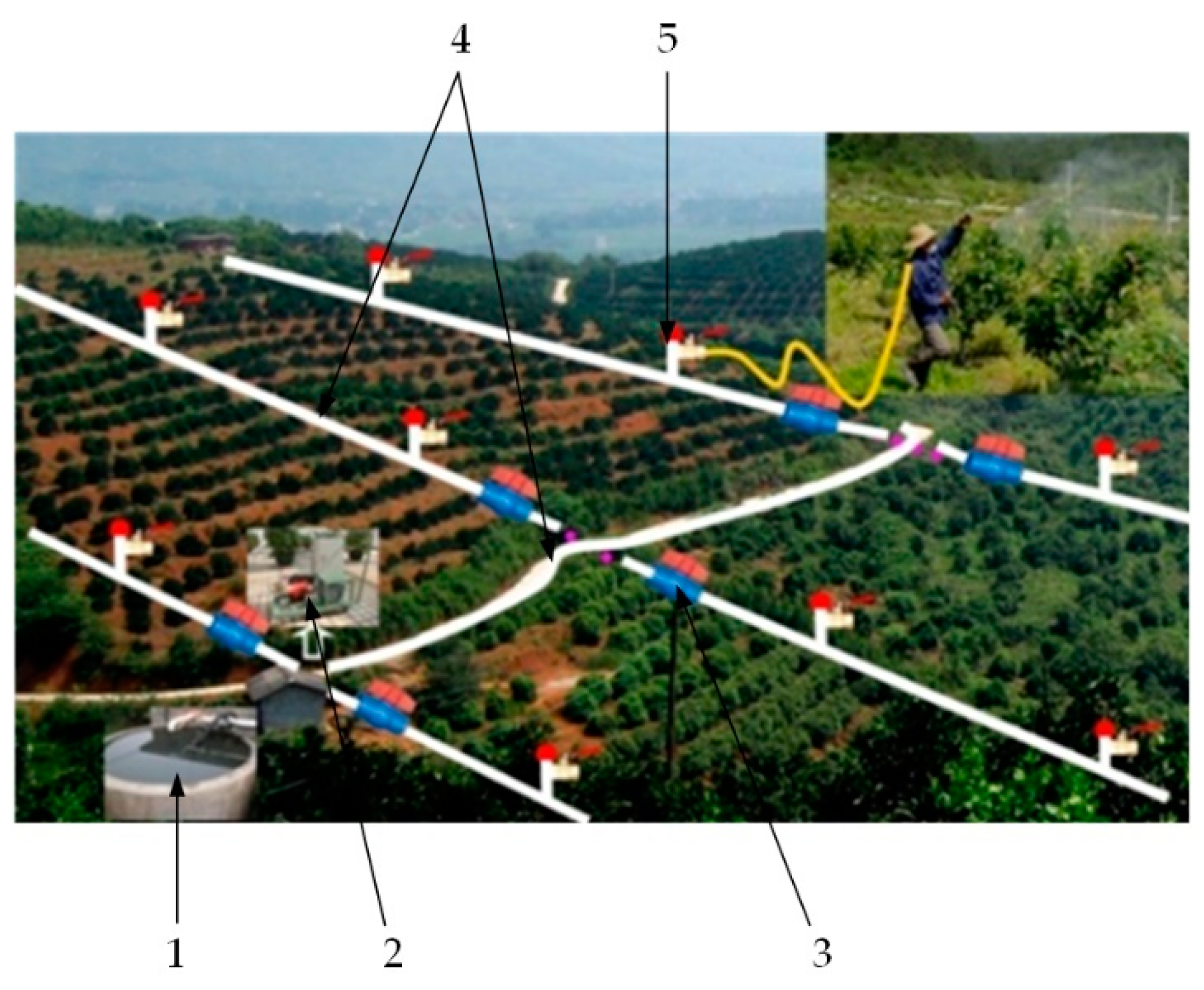
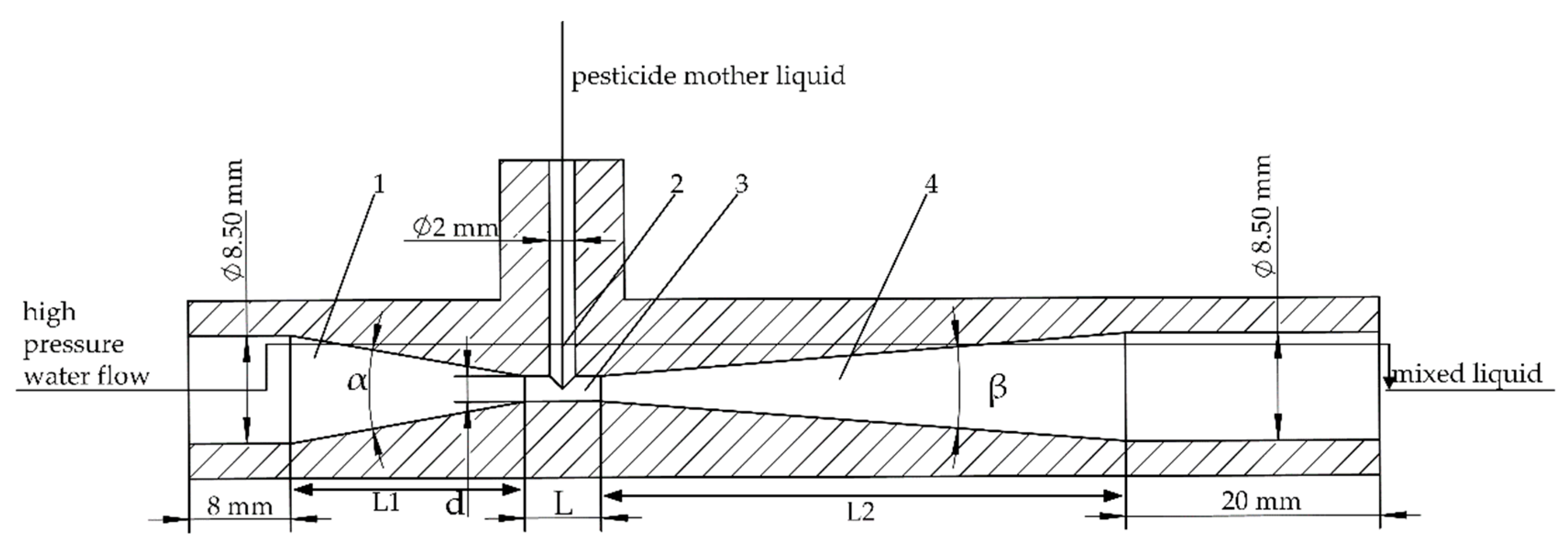
2.1.1. Design of Pesticide Mixing Apparatus Basic Structure

Jet-mixing apparatus is characterized by no requirement of extra power, compact structure, convenient operation, and low cost. Compared with other pesticide mixing apparatus, jet-mixing apparatus has the advantages of strong mixing, reliable working performance, quick mixing, and so on [1,2]. Therefore, the mixing principle of jet-mixing apparatus is adopted as reference in the paper; the actual dimension of hose diameter in pipeline spraying is combined to design the basic structure of on-line pesticide mixing apparatus based on pipeline spraying, as shown in Figure 2. Here, the diameter of water inlet and mixture outlet is 8.5 mm, the diameter of the pesticide mother liquid inlet is 2 mm, and the diameter is matched with the dimension of the spray gun hose in practical application at a flow rate of 10 L/min in the corresponding size; the length of the constricted tube L1 is 15 mm, the length of the diffusion tube L2 is 42 mm.

The on-line pesticide mixing apparatus based on pipeline spraying is mainly composed of a constricted tube, suction chamber, Venturi, and diffusion tube, where the constricted tube falloff angle α, diffusion tube divergence angle β, Venturi diameter d, and Venturi length L are four key structure parameters of the on-line pesticide mixing apparatus; these parameters have an important influence on pesticide mixing performance [13,30,31]. Figure 2 shows that the velocity of high-pressure water flow penetrating through the constricted tube with a gradually reduced cross section area is gradually increased. Kinetic energy is increased, and pressure is gradually decreased, which is injected from the constricted tube outlet into the Venturi. Negative pressure is formed in the Venturi; the pesticide mother liquid in the dosing tank is entrained from the suction chamber to the pesticide mixing apparatus under the effect of barometric pressure, and it can exchange energy with the high-pressure water flow in the Venturi, where they are gradually and evenly mixed. Then, mixed liquid enters into the diffusion tube with a gradually increased cross section area. The velocity is gradually reduced, pressure is gradually increased, and the liquid flows out of the pesticide mixing apparatus outlet, thereby realizing online mixing of the pesticide mother liquid and water [6,7,32].

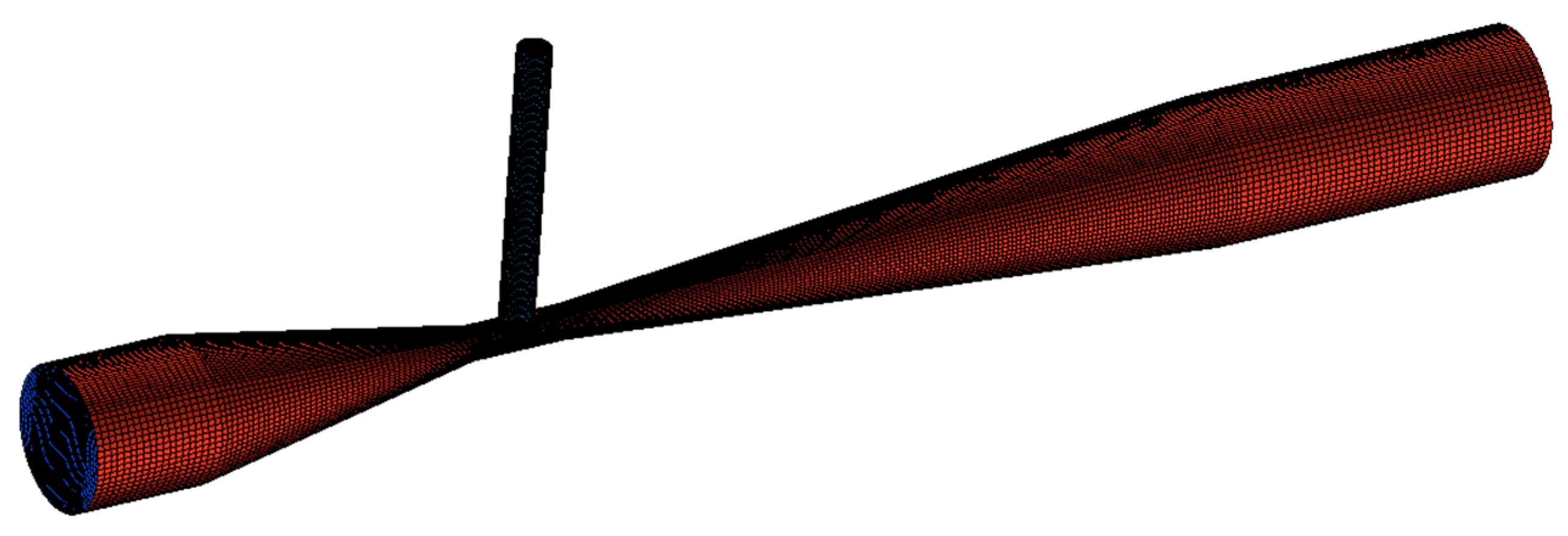
2.1.2. Establishment of Pesticide mixing Apparatus CFD Model

Before computational fluid dynamics (CFD) software Fluent is utilized for the numerical simulation calculation analysis of the on-line pesticide mixing apparatus internal flow field state on the basis of pipeline spraying, it is necessary to establish a CFD model for numerical simulation calculation. The pesticide mixing apparatus internal flow channel undergoes mesh generation through the integrated computer engineering and manufacturing code for computational fluid dynamics (ICEMCFD) mesh generation software in the paper, thereby generating a CFD model in line with requirements.

The pesticide mixing apparatus internal flow channel has a regular geometrical shape. Structure-based meshes can be adopted for division, thereby reducing mesh quantity and improving the numerical simulation calculation speed. Meshes vertical to the flowing direction can be easily generated by structure-based hexahedral mesh generation technology, thereby reducing pseudo diffusion, improving CFD model mesh quality, and ensuring computational accuracy. In the paper, structure-based hexahedral mesh is adopted for mesh generation in the pesticide mixing apparatus internal flow channel computational domain [33,34,35]. Since all structures of the pesticide mixing apparatus internal flow channel are basically circular tube sections, advanced O-shaped mesh generation technology of ICEMCFD is adopted, and blocks for generating structure-based hexahedral mesh are divided into an O-shape, thereby facilitating the generation of a CFD model with higher mesh quality, and improving the computational accuracy.

Normal velocity has very large gradients in areas close to the pesticide mixing apparatus internal flow channel wall, flow field conditions are complex, and standard wall-function method can be adopted for correct solution of the simulation value model wall condition according to CFD software Fluent. Six boundary layers are arranged in the pesticide mixing apparatus internal flow channel wall area for mesh encryption processing, thereby meeting numerical calculation requirements. The pesticide mixing apparatus internal flow channel suction chamber, Venturi, and areas with more complicated diffusion tube flow field states undergo local mesh encryption processing in order to evaluate pesticide mixing apparatus pesticide dissolution performance and pesticide mixing performance more accurately. In this process, 160 nodes are arranged on each longitudinal block line in suction chamber, 40 nodes are arranged on each transverse block line of each Venturi, and 150 nodes are arranged on each oblique block line of diffusion tube, thereby improving the computational accuracy, and better reflecting the pesticide mixing apparatus internal flow field state. A CFD model in line with numerical calculation requirements can be finally generated, as shown in Figure 3, and the mesh quantity is 416,160.

2.2. Design of Orthogonal Experiment

2.2.1. Design of Orthogonal Experiment Plan

When medium and large plant protection machinery for field crop are used for spraying operations, better spraying effect can be achieved when the spraying pressure is 1 to 2 MPa. On the contrary, if the spraying object is a fruit tree hillside orchard, higher spraying pressure is required during pipeline spraying operations, which should be higher than 0.8MPa generally; this allows a pronounced spraying effect to be achieved [36]. Many field experiment studies show that excellent spraying effect can be achieved when the pipeline spraying operation spraying pressure is 1 MPa. Document literature is consulted, and it is obvious that pressure loss of jet-mixing apparatus is higher than or equal to 50% [6,10,13,14,31]. Therefore, the analysis method based on CFD orthogonal experiment is adopted in the paper, high pressure water flow inlet pressure of pipeline spraying on-line pesticide mixing apparatus is set as 2 MPa, pesticide mother liquid inlet pressure is set as 0 MPa (barometric pressure), mixed liquid outlet pressure is set as 1 MPa.

The use of the double dilution method for the concentration formulation of pharmaceutical solutions improves the dispersion and suspension of the active ingredients and allows for more accurate dosing. In order to make it easier and more intuitive for the subsequent operator to use the on-line mixing device based on pipeline spraying, the article uses a multiplicative representation for the preparation of a certain concentration of liquid. By consulting relevant information on pesticides on websites such as China Pesticide First and China Pesticide Network, it was determined that the mixing ratio of most pesticide stock solutions to water was between 1:200 and 1:4000, i.e., the dilution times were between 200 and 4000 times. In the whole process of preparing the concentration of the liquid, the mother liquor dilution method firstly dilutes the pesticide stock solution by 2 to 20 times to make the pesticide mother liquor, and then the pesticide mother liquid is mixed by the on-line mixing device, i.e., the pesticide is diluted by 100 to 200 times to spray. Ultimately, the pesticide stock solution can be diluted 200 to 4000 times to meet the needs of most pesticide dilutions. Therefore, the mixing ratio of the pesticide mother liquid and water in the online mixing device based on pipeline spraying designed in this paper is finally determined as 1:100~1:200.

The pesticide mixing apparatus internal flow field state is studied and analyzed to observe the influence of change of four key structure parameters on pesticide mixing apparatus pesticide dissolution performance and pesticide mixing performance; the four parameters include constricted tube falloff angle α, diffusion tube divergence angle β, Venturi diameter d, and Venturi length L, thereby finally discovering the comprehensive optimal pesticide mixing apparatus structure parameters.

Change in single structure parameters affects pesticide mixing apparatus pesticide dissolution performance and pesticide mixing performance. Therefore, some interaction thereof also can generate a certain influence on pesticide mixing apparatus pesticide dissolution performance and pesticide mixing performance according to the above four key structure parameters, and a main influence can be determined. Therefore, four principal factors and three interaction factors are finally selected as experiment factors based on CFD orthogonal experiment study in the paper. The four principal factors are the constricted tube falloff angle α (factor A), diffusion tube divergence angle β (factor B), Venturi diameter d (factor C), and Venturi length L (factor D); the three interaction factors are the interaction between constricted tube falloff angle α and diffusion tube divergence angle β (factor A*B), interaction between diffusion tube divergence angle β and Venturi diameter d (factor B*C), as well as the interaction between diffusion tube divergence angle β and Venturi length L (factor B*D).

2.2.2. Experiment Evaluation Indexes and Factor Level

Before the orthogonal experiment table is designed, suitable factor levels should be firstly selected for four principal factors in orthogonal experiment; the factor level is finally selected in the paper as

Table 1. Factor level table.

Level	Factor
	A	B	C	D
	α/ (°)	β/ (°)	d/mm	L/mm
1	0.884	0.626	3.058	0.888
2	1.189	1.078	0.268	1.200
3	1.318	1.688	0.066	1.303

A = constricted tube falloff angle α; B = diffusion tube divergence angle β; C = Venturi diameter d; D = Venturi length L.

based a large number of literature [1,14,26,34] and previous pre-experiment study results.

Three experiment evaluation indexes are selected for evaluation in the paper in order to correctly evaluate pesticide mixing apparatus pesticide dissolution performance and pesticide mixing performance, respectively, including lifting height H₁, turbulent kinetic energy k, and pressure recovery distance H₂, wherein lifting height evaluation indexes is used for evaluating pesticide mixing apparatus pesticide dissolution performance, and turbulent kinetic energy evaluation indexes and pressure recovery distance evaluation indexes are jointly used for evaluating pesticide mixing apparatus pesticide mixing performance. The influence of three experiment evaluation indexes on pesticide mixing apparatus pesticide dissolution performance and pesticide mixing performance is concretely described as follows:

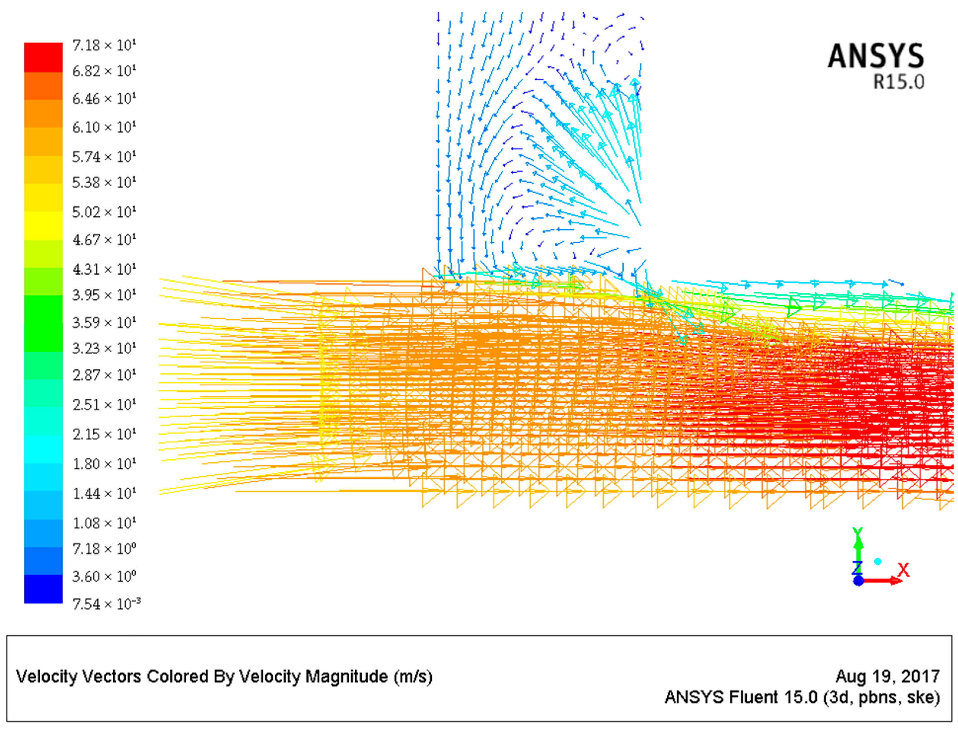
• Lifting heigh: the pesticide dissolution performance of the pesticide mixing apparatus is evaluated through observing the velocity vector diagram of the suction chamber traverse section, and recording the maximum height numerical value of high pressure water flow rising in the suction chamber. If the maximum height of high pressure water flow rising is lower, the obstruction of rising high pressure water flow to the sucked pesticide mother liquid is smaller, and the pesticide dissolution performance is better.
• Turbulent kinetic energy: the numerical value of the maximum turbulent kinetic energy reached by the pesticide mixing apparatus internal flow field is observed and recorded for measuring the mixing ability of the pesticide mixing apparatus. If the maximum turbulent kinetic energy is higher, the pesticide mixing apparatus internal flow field turbulence development is better, the flow field state is more unstable, the water and pesticide mother liquid can be mixed better, and the mixing ability is stronger.
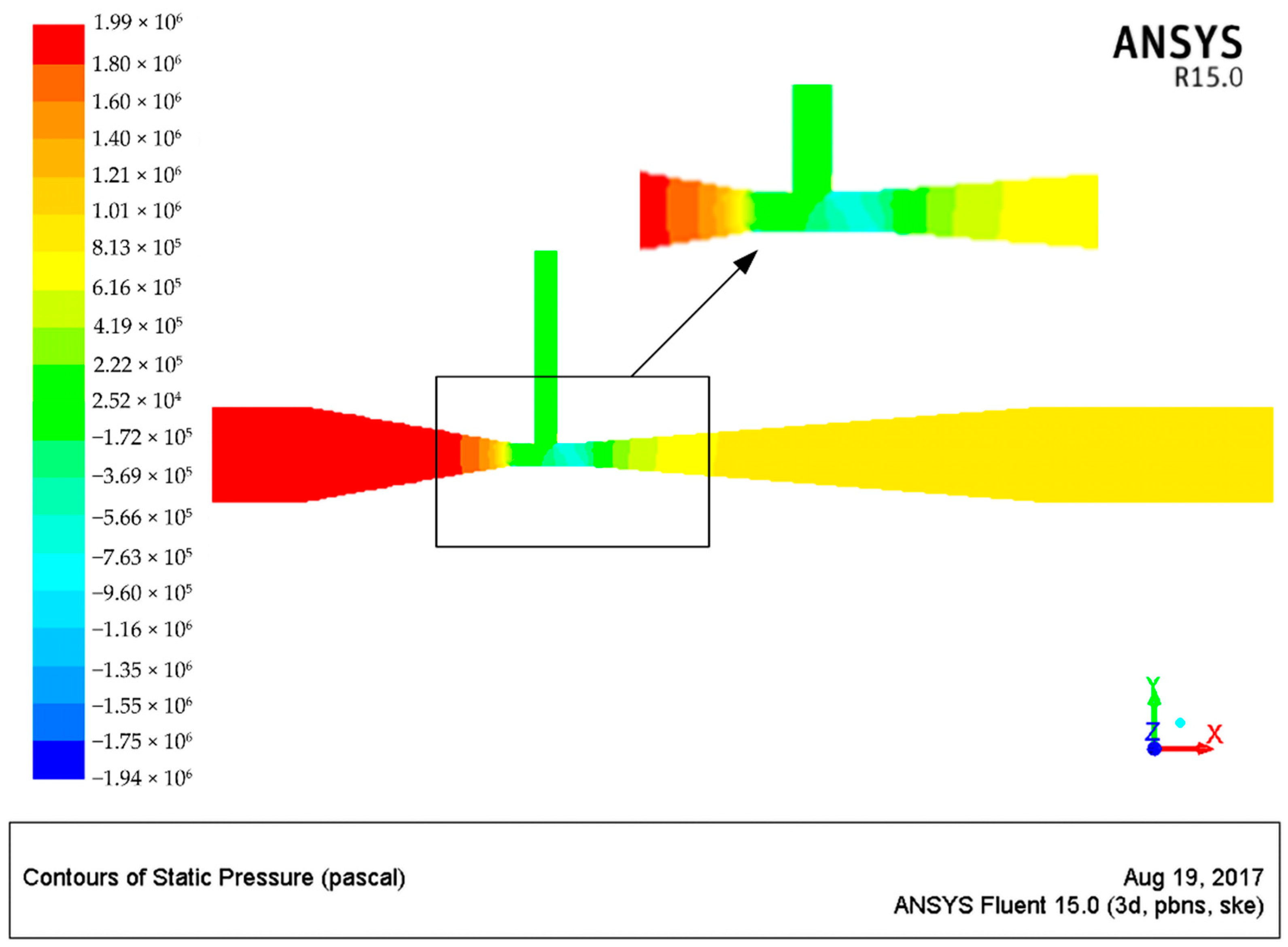
• Pressure recovery distance: the distance for increasing the diffusion tube internal pressure from 0.1 MPa to 0.9 MPa is observed and recorded for measuring the pressure recovery ability of the pesticide mixing apparatus. If the distance is shorter, the pressure recovery is faster, the pressure recovery ability is stronger, and the pressure loss is smaller.

2.2.3. Design of Orthogonal Experiment Table

Since each principal factor contains three levels, the degree of freedom (DOF) of each column in the orthogonal experiment table is 2, the DOF of each interaction factor is 4, and each interaction should occupy two columns in the orthogonal experiment table. Therefore, the column number of factor A*B in the orthogonal experiment table is, respectively, AB1 and AB2, the column number of factor B*C is, respectively, BC1 and BC2, and the column number of factor B*D is, respectively, BD1 and BD2. Three error columns with column numbers of E1, E2, and E3, respectively, also should be finally reserved, and they are used for estimating random errors. An interaction orthogonal table with a table head of L27(313) is selected in the paper accordingly [28]. SPSS data statistical analysis software is utilized for generating the orthogonal experiment table in line with experiment requirements, as can be seen in

Table 2. Orthogonal experiment table.

Experiment Number	Column Number
	A	B	AB1	AB2	C	BD2	E1	BC1	D	E2	BC2	BD1	E3
1	2	2	3	2	3	2	3	1	1	3	1	1	3
2	1	2	1	3	3	3	3	2	3	2	2	1	1
3	2	1	3	3	1	3	1	3	2	2	3	1	3
4	3	2	2	1	3	1	3	3	2	1	3	1	2
5	3	2	1	3	2	1	1	3	1	3	2	2	3
6	2	2	2	1	2	2	1	1	3	2	3	2	1
7	2	3	2	3	1	1	3	2	2	3	1	2	1
8	1	1	3	3	3	1	2	1	3	3	3	2	2
9	3	1	1	1	3	2	2	2	2	2	1	2	3
10	1	3	3	1	1	2	3	3	1	2	2	2	2
11	3	3	1	2	1	3	3	1	3	1	3	2	3
12	2	2	1	3	1	2	2	1	2	1	2	3	2
13	2	3	1	2	3	1	1	2	1	2	3	3	2
14	1	2	2	1	1	3	2	2	1	3	3	3	3
15	1	1	2	2	2	1	3	1	2	2	2	3	3
16	2	1	1	1	2	3	3	3	3	3	1	3	2
17	3	1	3	3	2	2	3	2	1	1	3	3	1
18	3	3	2	3	2	3	2	1	1	2	1	1	2
19	1	3	2	3	3	2	1	3	3	1	1	3	3
20	2	3	3	1	2	1	2	2	3	1	2	1	3
21	1	2	3	2	2	3	1	2	2	1	1	2	2
22	3	2	3	2	1	1	2	3	3	2	1	3	1
23	2	1	2	2	3	3	2	3	1	1	2	2	1
24	1	3	1	2	2	2	2	3	2	3	3	1	1
25	1	1	1	1	1	1	1	1	1	1	1	1	1
26	3	1	2	2	1	2	1	2	3	3	2	1	2
27	3	3	3	1	3	3	1	1	2	3	2	3	1

A = constricted tube falloff angle α; B = diffusion tube divergence angle β; C = Venturi diameter d; D = Venturi length L; ABX = the column number of factor A*B in orthogonal experiment table (X = 1, 2); BCX = the column number of factor B*C in orthogonal experiment table (X = 1, 2); BDX = the column number of factor B*D in orthogonal experiment table (X = 1, 2); EX = error columns (X = 1, 2, 3).

.

2.3. Boundary Condition and Model Selection

Fluent software is adopted for computational fluid dynamics (CFD) numerical analog simulation research and analysis on pesticide mixing apparatus internal flow field state in the paper: high pressure water flow inlet boundary is set as pressure inlet, gauge pressure is 2 MPa; pesticide mother liquid inlet boundary is set as pressure inlet, gauge pressure is 0 MPa; mixed liquid outlet boundary is pressure outlet, gauge pressure is 1 MPa. Non-slipping wall boundary condition is adopted for the wall, standard wall-function method is adopted for treating the area near the wall, and operating environment belongs to standard barometric pressure [13,14,26,37].

The standard k-ε two-equation turbulence model belongs to a turbulence model, which is applied most widely in the engineering field at present. This can be better applied in a complex 3D flow field, and it is physically meshed in the aspect of flow field simulation with a lower calculated amount and rational precision. The model is economical and practical [1,10,13,26,31,33,38,39]. Therefore, a standard k-ε two-equation turbulence model is adopted for numerical simulation solution calculations on the CFD model in the paper.

Turbulent kinetic energy k equation:

$$\frac{\partial }{{\partial }_t}\left(\rho k\right)+div\left(\rho \mu k\right)=div\left[\left(\mu +\frac{{\mu }_t}{{\sigma }_k}\right)\times grad\left(k\right)\right]-\rho \epsilon +{\mu }_t{P}_G$$

(1)

Turbulent dissipation rate ε equation:

$$\frac{\partial }{{\partial }_t}\left(\rho \epsilon \right)+div\left(\rho \mu \epsilon \right)=div\left[\left(\mu +\frac{{\mu }_t}{{\sigma }_z}\right)\times grad\left(\epsilon \right)\right]-\rho C_2\frac{{\epsilon }^2}{k}+{\mu }_t{C}_1\frac{\epsilon }{k}{P}_G$$

(2)

In the above formula: k is the turbulent kinetic energy in m²·s⁻², ε is the turbulent dissipation rate in m²·s⁻³, ρ is the fluid density in kg·m⁻³, μ is the dynamic coefficient of viscosity in kg·m⁻¹·s⁻¹, μ_t is the turbulence coefficient of viscosity in kg·m⁻¹·s⁻¹, and P_G is the turbulent kinetic energy generation item in s⁻².

SIMPLEC algorithm is adopted for pressure velocity coupling solution, PRESTO interpolating scheme is adopted for pressure equation solution in the aspect of solving method, other equation solutions are dispersed through Second Order Upwind method, residual error convergence standard is set as 1 × 10⁻⁴, and Hybird Initialization is adopted for initialization [11,26,34,40].

Concrete steps of numerical simulation calculation are shown as follows:

• Fluent solver selection;
  3DFluent solver should be selected according to the pesticide mixing apparatus model.
• Mesh importing;
  Menu bar File→Read→Mesh options are selected, and then msh files exported from ICEM software are selected.
• Mesh checking;
  Menu bar Mesh→Check options are selected, and the operator should observe whether meshes suffer from negative volume. Meshes are divided again if there is negative volume.
• Setting of computational domain dimensions;
  Since the basic unit of the pesticide mixing apparatus internal flow channel CFD model is mm, and the basic unit of Fluent software is m, it is necessary to select the menu bar Mesh→Scale options for setting the imported model as mm.
• Selection of calculation model;
  Pressure-Based solver is selected for General parameter setting panel. Steady stable-state flow is selected for the panel Time option. Viscous-Standard k-e is used for standing the Models parameter setting panel, namely standard k-ε two-equation model.
• Confirmation of fluid physical properties;
  Water-liquid is selected in the material depot equipped for the Fluent software; namely liquid water is regarded as the working liquid material.
• Definition of operating environment;
  Menu bar Define→Operating Conditions option is selected, 101325 is the input into the Operating Pressure textbox, as the operating environment namely has standard barometric pressure.
• Appointment of boundary condition;
  In the Boundary Conditions parameter settings panel, high pressure water flow inlet is set as pressure inlet, gauge pressure is 2 MPa, pesticide mother liquid inlet is set as pressure inlet, and gauge pressure is 0 MPa; mixed liquid outlet is set as pressure outlet, and gauge pressure is 1 MPa.
• Solving method setting;
  Th pressure velocity coupling solution algorithm of SIMPLEC algorithm is set in the Solution Methods parameter setting panel, PRESTO interpolating scheme is adopted for pressure equation solution, and other equation solutions are dispersed by Second Order Upwind method.
• Solution monitoring setting;
  Residual error convergence standard of 1 × 10⁻⁴ is set for Monitors parameter settings panel. One monitoring face is established for monitoring the change of mixture outlet mass flow rate.
• Flow field initialization;
  Hybird Initialization is adopted for initializing flow field in the Solution initialization parameter settings panel.
• Iterative solution;
  Iteration frequency of 4000 is set as the Run Calculation parameter settings panel to start the numerical simulation calculation.
• Result checking.
• Result saving and after-treatment.

3. Results and Discussion

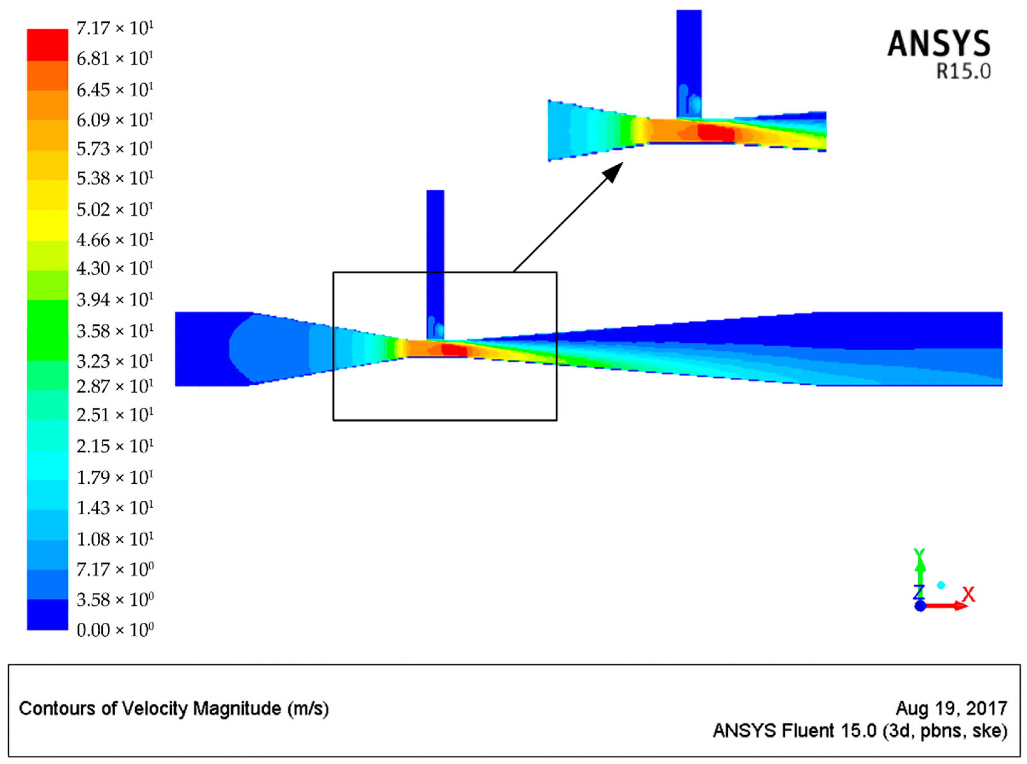
3.1. Analysis of Chemical Mixer Internal Flow Field

Table 1 and Table 2 in the paper, as well as setting in text 2.3, are used for the numerical calculation of the pesticide mixing apparatus internal flow field; calculation results occupy a large amount of written space. Experiment number 10 is only listed in the paper. The pesticide mixing apparatus internal flow field numerical calculation results for constricted tube falloff angle is 20°, diffusion tube divergence angle is 9°, Venturi diameter is 2 mm, and Venturi length is 6 mm, as shown in Figure 4, Figure 5 and Figure 6.

Figure 4 and Figure 5 are combined. It is obvious that as low velocity high pressure water flow penetrates through the constricted tube with a gradually decreased cross section area, velocity is gradually increased, pressure is gradually decreased, and it is changed into a high-velocity low pressure water flow. Velocity reaches its maximum value in the Venturi, and pressure reaches the minimum level, thereby forming negative pressure; the pesticide mother liquid is sucked from the suction chamber into the pesticide mixing apparatus under the effect of the strong external barometric pressure and static pressure of the liquid. Two liquid flows with different velocities exchange energy in the Venturi, water flow rate is reduced, the flow rate of pesticide mother liquid is increased, and they are gradually and evenly mixed. Since the cross-section area of the diffusion tube is gradually increased, some kinetic energy is converted into pressure energy, mixed liquid flow rate is gradually decreased, and pressure is gradually increased, which is accompanied by certain velocity layering. Zhou et al. [13] have also concluded that the cross-sectional area can influence the suction performance of the mixing device, and that the best suction performance can be achieved with an area ratio between 1.0 and 1.6, but that the suction performance will gradually deteriorate when the area ratio exceeds 2.0.

Figure 6 shows that some velocity vectors of backflow suction chambers and local vortexes appear at the joint of the suction chamber and Venturi, which produces a certain influence on the phytosanitary dissolution performance of the chemical mixer. However, the velocity vectors are changed from a higher value to lower value with the increase of the suction chamber height, which is gradually attenuated, and finally changed into a completely downward velocity vector. It is obvious that the pesticide mother liquor can be smoothly sucked, since upward water flow has a smaller suction influence on the pesticide mother liquor.

3.2. Orthogonal Experiment Results and Analysis

3.2.1. Orthogonal Experiment Data

The CFD model of all experiment numbers in orthogonal experiment Table 2 undergoes numerical simulation calculation, and the performance evaluation indexes experiment data of the pesticide mixing apparatus under different experiment numbers is shown as

Table 3. Orthogonal experiment data table.

Experiment Number	Evaluation Indexes
	Lifting Height H1/mm	Turbulent Kinetic Energy k/m2·s−2	Pressure Recovery Distance H2/mm
1	0.07	302.45	24.97
2	0.06	279.09	24.81
3	1.88	239.12	17.62
4	0.05	292.47	24.68
5	0.24	266.51	20.57
6	0.20	239.33	20.58
7	4.84	287.50	15.02
8	0.05	316.23	25.72
9	0.05	315.28	25.63
10	3.58	281.30	15.21
11	5.27	285.64	14.83
12	3.05	266.88	16.16
13	0.10	299.32	24.70
14	2.41	265.10	16.30
15	0.17	228.03	22.20
16	0.13	270.18	21.96
17	0.17	290.23	21.94
18	0.44	272.16	19.61
19	0.08	249.28	24.43
20	0.38	242.90	19.56
21	0.26	232.11	20.84
22	3.36	265.35	15.98
23	0.05	330.57	25.81
24	0.42	244.15	19.87
25	0.93	233.11	17.71
26	2.20	240.78	17.47
27	0.08	267.00	24.31

.

3.2.2. Analysis on Orthogonal Experiment Variance

The orthogonal experiment in the paper contains three evaluation indexes, which belong to the multi-index orthogonal experiment. Each evaluation index undergoes single-index variance analysis, respectively, in order to discover the main influence factors and comprehensive optimal pesticide mixing apparatus structure parameters; the optimal level of each evaluation index is determined. Next, analysis results of all evaluation indexes are comprehensively considered and analyzed according to the experiment purpose; the comprehensive optimal level is finally determined, and comprehensive optimal pesticide mixing apparatus structure parameters are discovered. Results data of all variance analysis and all factor level data mean values calculated by SPSS data statistical analysis software are shown in

Table 4. Lifting height variance analysis.

Variance Source	Quadratic Sum	DOF	Mean Square Error	F	p Value
A	0.891	2	0.446	2.549	0.158
B	5.115	2	2.557	14.628	0.005
C	50.335	2	25.168	143.952	0.000
D	0.843	2	0.421	2.410	0.171
A*B	0.060	4	0.015	0.085	0.984
B*C	7.611	4	1.903	10.883	0.006
B*D	0.048	4	0.012	0.068	0.989
error	1.049	6	0.175
Total	65.951	26

,

Table 5. All principal factor level data mean values of lifting height.

Level	Factor H1/mm
	A	B	C	D
1	0.884	0.626	3.058	0.888
2	1.189	1.078	0.268	1.200
3	1.318	1.688	0.066	1.303

A = constricted tube falloff angle α; B = diffusion tube divergence angle β; C = Venturi diameter d; D = Venturi length L.

,

Table 6. Variance analysis of turbulent kinetic energy.

Variance Source	Quadratic Sum	DOF	Mean Square Error	F	p Value
A	1875.760	2	937.880	8.731	0.017
B	167.241	2	83.620	0.778	0.501
C	8244.767	2	4122.383	38.376	0.000
D	1913.082	2	956.541	8.905	0.016
A*B	107.812	4	26.953	0.251	0.899
B*C	7260.973	4	1815.243	16.898	0.002
B*D	443.888	4	110.972	1.033	0.462
error	644.527	6	107.421
Total	20,658.050	26

,

Table 7. Data mean values matched with interaction factor B*C of turbulent kinetic energy, respectively.

Factor C Level	Factor B Level k/m2·s−2
	1	2	3
1	237.670	265.777	284.813
2	262.813	245.983	253.070
3	320.693	291.337	271.867

,

Table 8. All principal factor level data mean values of turbulent kinetic energy.

Level	Factor k/ m2·s−2
	A	B	C	D
1	258.711	273.726	262.753	282.306
2	275.361	267.699	253.956	263.616
3	277.269	269.917	294.632	265.420

A = constricted tube falloff angle α; B = diffusion tube divergence angle β; C = Venturi diameter d; D = Venturi length L.

,

Table 9. Analysis of pressure recovery distance variance.

Variance Source	Quadratic Sum	DOF	Mean Square Error	F	p Value
A	0.246	2	0.123	16.311	0.004
B	19.325	2	9.663	1282.019	0.000
C	344.774	2	172.387	22,872.018	0.000
D	0.126	2	0.063	8.380	0.018
A*B	0.004	4	0.001	0.122	0.969
B*C	1.558	4	0.389	51.676	0.000
B*D	0.014	4	0.004	0.474	0.755
error	0.045	6	0.008
Total	366.093	26

and

Table 10. All principal factor level data mean values of pressure recovery distance.

Level Levels	Factor H2/mm
	A	B	C	D
1	20.788	21.784	16.256	20.758
2	20.709	20.543	20.792	20.703
3	20.558	19.727	25.007	20.593

A = constricted tube falloff angle α; B = diffusion tube divergence angle β; C = Venturi diameter d; D = Venturi length L.

.

Variance analysis F test in Table 4 shows that p value of factor B, factor C, and interaction factor B*C is smaller than 0.05, and p value of factor A, factor D, interaction factor A*B, and interaction factor B*D is larger than 0.05. Therefore, factor B, factor C, and interaction factor B*C have significant influence on lifting height evaluation indexes at significance level α = 0.05, and factor A, factor D, interaction factor A*B, and interaction factor B*D have insignificant influence difference on lifting height evaluation indexes. The primary and secondary influence sequences of all factors on lifting height can be discovered, namely C > B > B*C > A > D > A*B > B*D. Table 5 shows that the optimal level of lifting height evaluation indexes is A₁B₁C₃D₁, namely, the constricted tube falloff angle is 20°, diffusion tube divergence angle is 7°, Venturi diameter is 3 mm, and Venturi length is 6 mm.

The variance analysis F test in Table 6 shows that p value of factor A, factor C, factor D, and interaction factor B*C is smaller than 0.05, and the p value of factor B, interaction factor A*B, and interaction factor B*D is larger than 0.05. Therefore, factor A, factor C, factor D, and interaction factor B*C have significant influence on turbulent kinetic energy evaluation indexes at the significance level α = 0.05, and factor B, interaction factor A*B, and interaction factor B*D have insignificant influence difference on turbulent kinetic energy evaluation indexes. The primary and secondary influence sequences of all factors on turbulent kinetic energy can be discovered, namely C > B*C > D>A > B*D > B>A*B. Since the diffusion tube divergence angle β is matched with Venturi diameter d, the interaction thereof has significantly greater influence on turbulent kinetic energy evaluation indexes than that on principal factor diffusion tube divergence angle β. Therefore, the optimal level of two structure parameters of diffusion tube divergence angle β and Venturi diameter d should be determined by their matched interaction optimal level. Table 7 and Table 8 show that the optimal level of turbulent kinetic energy evaluation indexes is A₃B₁C₃D₁, namely, the constricted tube falloff angle is 22°, diffusion tube divergence angle is 7°, Venturi diameter is 3 mm, and Venturi length is 6 mm.

Variance analysis F test of Table 9 shows that the p value of factor A, factor B, factor C, factor D, and interaction factor B*C is smaller than 0.05, and the p value of interaction factor A*B and interaction factor B*D is larger than 0.05. Therefore, factor A, factor B, factor C, factor D, and interaction factor B*C have significant influence on pressure recovery distance evaluation indexes at significance level α = 0.05, and interaction factor A*B and interaction factor B*D have insignificant influence difference on pressure recovery distance evaluation indexes. The primary and secondary sequences of all factors on pressure recovery distance is discovered, namely C > B > B*C > A>D > B*D > A*B. Table 10 shows that optimal level of pressure recovery distance evaluation indexes is A₃B₃C₁D₃, namely, constricted tube falloff angle is 22°, diffusion tube divergence angle is 9°, Venturi diameter is 2 mm, and Venturi length is 10 mm.

3.2.3. Determination of Comprehensive Optimal Level of Chemical Mixer Structure Parameters

When the influence of factor on indexes is analyzed, if single-index is available only under general conditions, interaction among factors is not considered, the optimal levels of all factors are combined, and it is regarded as the optimal optimization grouping. However, three evaluation indexes are considered for orthogonal experiment in the paper, and the experiment is thus a multi-index orthogonal experiment. The experiment results of the three evaluation indexes should be considered, respectively, and the analysis results of all evaluation indexes also should be considered and analyzed comprehensively according to experiment objectives, so that the comprehensive optimal level is finally determined. The orthogonal experiment in the paper aims at improving the pesticide mixing performance as much as possible, whilst guaranteeing that the pesticide dissolution performance is acceptable. Therefore, two evaluation indexes of turbulent kinetic energy and pressure recovery distance should be comprehensively considered first; it should be ensured that lifting height evaluation indexes are not too high, and that they are acceptable. The following are set: lifting height evaluation indexes account for 20%, turbulent kinetic energy evaluation indexes account for 40%, and pressure recovery distance evaluation indexes account for 40%. Finally, the determined comprehensive optimal level is A₃B₃C₁D₁, and through comprehensive consideration and analysis according to weight, the constricted tube falloff angle is 22°, diffusion tube divergence angle is 9°, Venturi diameter is 2 mm, and Venturi length is 6 mm.

3.2.4. Verification of Chemical Mixer Structure Parameter Comprehensive Optimal Level

Finally, the determined comprehensive optimal level combination is arranged in the orthogonal experiment of the paper; the combination should undergo a verification experiment, thereby proving that it is the comprehensive optimal level of the orthogonal experiment in the paper. The pesticide mixing apparatus internal flow channel simulation value model of combination structure parameters undergoes numerical simulation calculation analysis, and it is concluded that the lifting height is 3.79 mm, turbulent kinetic energy is 299.42 m²·s⁻², and pressure recovery distance is 14.93 mm; the experiment number is recorded as experiment 28. In order to prove that the determined comprehensive optimal level combination adheres to the comprehensive optimal pesticide mixing apparatus structure parameters, it is necessary to comprehensively score and calculate 27 groups of experiment results and the experiment results of experiment No. 28 in Table 3, according to the determined weight. When the comprehensive score of experiment No. 28 is the highest, it is obvious that the determined comprehensive optimal level combination adheres to the comprehensive optimal pesticide mixing apparatus structure parameters.

Since all evaluation indexes have great magnitude order difference, it is necessary to first normalize primary data of all evaluation indexes; the result values can be mapped in the interval [0, 1]. Min-max dispersed standardized method is adopted in the paper for normalizing primary data of all evaluation indexes, and the computational formula is shown in Formulas (3)–(5).

$$x^{*}=\frac{x-{\min }_x}{{\max }_x-{\min }_x}$$

(3)

In the formula: x* is the value of lifting height evaluation index primary data after normalization, x is the lifting height evaluation index primary data in mm, min_x is the minimum value of lifting height evaluation indexes data in mm, max_x is the maximum value of lifting height evaluation indexes data in mm.

$$y^{*}=\frac{y-{\min }_y}{{\max }_y-{\min }_y}$$

(4)

In the formula: y* is the value of turbulent kinetic energy evaluation index primary data after normalization, y is the turbulent kinetic energy evaluation index primary data in m²·s⁻², min_y is the minimum value of turbulent kinetic energy evaluation indexes data in m²·s⁻², max_y is the maximum value of turbulent kinetic energy evaluation indexes data in m²·s⁻².

$$z^{*}=\frac{z-{\min }_z}{{\max }_z-{\min }_z}$$

(5)

In the formula: z* is the value of pressure recovery distance evaluation index primary data after normalization, z is the pressure recovery distance evaluation index primary data in mm, min_z is the minimum value of pressure recovery distance evaluation indexes data in mm, max_z is the maximum value of pressure recovery distance evaluation indexes data in mm.

Since the results of two evaluation indexes of lifting height and pressure recovery distance are smaller and better, results of turbulent kinetic energy evaluation indexes are higher and better. In order to facilitate subsequent correct and comprehensive scoring calculation and comparison, number 1 is respectively subtracted by the value of two evaluation indexes of lifting height or pressure recovery distance after primary data normalization, and these values are respectively regarded as the two evaluation index final normalization results; the computational formula is shown in Formulas (6) and (7). Formula (4) is still adopted for turbulent kinetic energy evaluation index final normalization results.

$$x^{\prime }=1-x^{*}$$

(6)

In the formula: x′ is the lifting height evaluation index final normalization results, x^* is the normalization result of lifting height evaluation indexes calculated through Formula (3).

$$z^{\prime }=1-z^{*}$$

(7)

In the formula: z′ is the pressure recovery distance evaluation index final normalization results, z* is the normalization result of pressure recovery distance evaluation indexes calculated through Formula (5).

The comprehensive score concrete computational formula can be obtained as shown in Formula (8) according to the above-mentioned proportion of all evaluation indexes:

$$cs=0.2x^{\prime }+0.4y^{*}+0.4z^{\prime }$$

(8)

In the formula: cs is the comprehensive score value of the calculation, x′ is the final normalization result of the lifting height evaluation index, y* is the final normalization result of the turbulent kinetic energy evaluation index, z′ is the index final normalization result of the pressure recovery distance evaluation.

In Formulas (3)–(8): primary data of all evaluation indexes are normalized, and the comprehensive score is finally calculated. The obtained evaluation index final normalization results and comprehensive score results of the pesticide mixing apparatus under different experiment numbers are shown in

Table 11. Normalization results and comprehensive score results.

Experiment Number	Evaluation Indexes			Comprehensive Score
	Lifting Height H1/mm	Turbulent Kinetic Energy k/m2·s−2	Pressure Recovery Distance H2/mm
1	0.996	0.726	0.077	0.520
2	0.998	0.498	0.091	0.435
3	0.649	0.108	0.746	0.472
4	1.000	0.628	0.103	0.493
5	0.964	0.375	0.477	0.534
6	0.971	0.110	0.476	0.429
7	0.082	0.580	0.983	0.642
8	1.000	0.860	0.008	0.547
9	1.000	0.851	0.016	0.547
10	0.324	0.520	0.965	0.659
11	0.000	0.562	1.000	0.625
12	0.425	0.379	0.879	0.588
13	0.990	0.695	0.101	0.517
14	0.548	0.362	0.866	0.601
15	0.977	0.000	0.329	0.327
16	0.985	0.411	0.351	0.502
17	0.977	0.607	0.352	0.579
18	0.925	0.430	0.565	0.583
19	0.994	0.207	0.126	0.332
20	0.937	0.145	0.569	0.473
21	0.960	0.040	0.453	0.389
22	0.366	0.364	0.895	0.577
23	1.000	1.000	0.000	0.600
24	0.929	0.157	0.541	0.465
25	0.831	0.050	0.738	0.481
26	0.588	0.124	0.760	0.471
27	0.994	0.380	0.137	0.406
28	0.284	0.696	0.991	0.732

, and the combination with the highest comprehensive score is the comprehensive optimal combination.

Table 11 shows that the comprehensive score of experiment No. 28 is prominently higher than the comprehensive scores of the remaining 27 groups of experiment combinations in Table 2. Therefore, it can be determined that it belongs to the comprehensive optimal level of orthogonal experiment in the paper.

According to the research, the best value of the contraction angle of the classical venturi structure is in the range of 20°~22° [41,42], and the optimal parameter of the contraction angle determined in the paper is 22°. With the increase of the contraction angle, the effective length of the contraction tube gets shorter, which can improve the mixing uniformity. The best value of the diffusion angle is in the range of 7°~14° [41], and the diffusion angle of 9° in the paper can achieve the uniformity of the pesticide mixing. Combined with related studies [43,44], it is found that the optimal structural parameters determined in the thesis are in line with objective laws, and the number of tests can be significantly reduced through orthogonal tests.

4. Conclusions

An analysis method based on CFD orthogonal experiment is adopted in the paper, thereby optimizing pesticide mixing apparatus structure parameters, effectively saving experiment costs, and reducing the need for experiment frequency. The following conclusions are made through numerical simulation calculation and orthogonal experiment variance analysis:

• Single-index variance analysis results show that diffusion tube divergence angle β and Venturi diameter d are the two structure parameters with the most important influence among the three experiment evaluation indexes, and the constricted tube falloff angle α and Venturi length L are two structure parameters with secondary influence. When it is only considered that turbulent kinetic energy is the evaluation index, interaction influence of diffusion tube divergence angle β and Venturi diameter d plays the decisive role, and the influence of interactions under other circumstances are from respective principal factors.
• Four structure parameters of pesticide mixing apparatus have different optimal values under different evaluation indexes. Optimal pesticide mixing apparatus structure parameters include the following when aiming at lifting height evaluation indexes: constricted tube falloff angle is 20°, diffusion tube divergence angle is 7°, Venturi diameter is 3 mm, and Venturi length is 6 mm; optimal pesticide mixing apparatus structure parameters include the following when aiming at turbulent kinetic energy evaluation indexes: constricted tube falloff angle is 22°, diffusion tube divergence angle is 7°, Venturi diameter is 3 mm, Venturi length is 6 mm; optimal pesticide mixing apparatus structure parameters include the following when aiming at pressure recovery distance evaluation indexes: constricted tube falloff angle is 22°, diffusion tube divergence angle is 9°, Venturi diameter is 2 mm, and Venturi length is 10 mm.
• Analysis results of all evaluation indexes are comprehensively considered to finally conclude the following comprehensive optimal pesticide mixing apparatus structure parameters: constricted tube falloff angle is 22°, diffusion tube divergence angle is 9°, Venturi diameter is 2 mm, and Venturi length is 6 mm.

References

1. Xu, Y.; Wang, X.; Zheng, J.; Zhou, F. Simulation and experiment on agricultural chemical mixing process for direct injection system based on CFD. Trans. Chin. Soc. Agric. Eng. 2010, 26, 148–152. [Google Scholar]
2. Li, J.; Jia, W.; Wei, X. On-line mixing pesticide device based on flow control valve and neural network. Trans. Chin. Soc. Agric. Mach. 2014, 45, 98–103. [Google Scholar]
3. Slaughter, D.; Giles, D.; Tauzer, C. Precision offset spray system for roadway shoulder weed control. J. Transp. Eng. 1999, 125, 364–371. [Google Scholar] [CrossRef]
4. Gillis, K.; Giles, D.; Slaughter, D.; Downey, D. Injection mixing system for boomless, target–activated herbicide spraying. Trans. ASAE 2003, 46, 997–1008. [Google Scholar] [CrossRef]
5. Liu, Z.; Xu, H.; Hong, T.; Zhang, W.; Zhu, Y.; Zhang, K. Key technology of variable-rate spraying system of online mixing pesticide. Trans. Chin. Soc. Agric. Mach. 2009, 40, 93–129. [Google Scholar]
6. He, P.; Wu, C.; Chen, C.; Li, X.; Wang, G. Experimental Investigation on Safe Mixing Apparatus. China Saf. Sci. J. 2001, 4, 38–42. [Google Scholar]
7. He, P.; Wu, C.; Chen, C.; Wang, G.; Li, X. Performance of a New Type Spraying mixing Apparatus. Trans. Chin. Soc. Agric. Mach. 2001, 3, 44–47. [Google Scholar]
8. Peijie, H.; Cuiying, C.; Chundu, W.; Xuehui, L. Numerical computation of mixing pipe flow-field in jet mixing apparatus pesticide mixture. J. Jiangsu Univ. Nat. Sci. Ed. 2002, 23, 13–16. [Google Scholar]
9. Li, Y.; Wu, C.; Fu, X. Experimental study on two-stage jet mixing apparatus. Trans. Chin. Soc. Agric. Eng. 2008, 1, 172–174. [Google Scholar]
10. Qiu, B.; Xu, X.; Deng, B.; Yang, N.; Jiang, G.; Wu, C. Effect of area ratio on mixing homogeneity in jet-mixing apparatus. Trans. Chin. Soc. Agric. Mach. 2011, 42, 95–100. [Google Scholar]
11. Qiu, B.; Xu, X.; Yang, N.; Deng, B.; Jiang, G.; Wu, C. Simulation analysis of structure parameters of jet-mixing apparatus on jet-mixing performance. Trans. Chin. Soc. Agric. Mach. 2011, 42, 70–69. [Google Scholar]
12. Chen, Z.; Zhu, S.; Qiu, B. Online jet mixing control system of pesticide concentration. J. Drain. Irrig. Mach. Eng. 2012, 30, 463–468. [Google Scholar]
13. Zhou, L.; Fu, X.; Xue, X. Design and experiment of jet mixing apparatus based on CFD. Trans. Chin. Soc. Agric. Mach. 2013, 44, 107–112. [Google Scholar]
14. Ou, M.; Jia, W.; Qiu, B.; Guan, X.; Sheng, Y. Experiment and numerical analysis of flow field in jet mixing device under variable working conditions. Trans. Chin. Soc. Agric. Mach. 2015, 46, 107–111. [Google Scholar]
15. Zhang, J.F.; Pang, X.B.; Liu, H.; Zhang, T.J.; Guo, X.; Zeng, F.C. Study on Proportional Control Experimental Platform of Online Jet Mixing Drug. Hubei Agric. Sci. 2016, 55, 2645–2648. [Google Scholar]
16. Ghate, S.R.; Phatak, S. A compressed air direct injection pesticide sprayer. Appl. Eng. Agric. 1991, 7, 158–162. [Google Scholar] [CrossRef]
17. Lin, M.; Zhao, G. Analysis for the security technology of chemical application in the plant protection mechinery from aborad. Trans. Chin. Soc. Agric. Mach. 1996, S1, 153–158. [Google Scholar]
18. Koo, Y.M.; Sumner, H. Total flow control for a direct injection sprayer. Appl. Eng. Agric. 1998, 14, 363–367. [Google Scholar] [CrossRef]
19. Steward, B.L.; Humburg, D. Modeling the raven scs-700 chemical injection system with carrier control with sprayer simulation. Trans. ASAE 2000, 43, 231–245. [Google Scholar] [CrossRef] [Green Version]
20. Aissaoui, A.E.; Lebeau, F.; Destain, M.F. Development of an optical sensor to measure direct injection spraying system performance. VDI-Ber. 2007, 2001, 243–252. [Google Scholar]
21. Luck, J.D.; Shearer, S.A.; Luck, B.D.; Payne, F.A. Evaluation of a rhodamine-WT dye/glycerin mixture as a tracer for testing direct injection systems for agricultural sprayers. Appl. Eng. Agric. 2012, 28, 643–646. [Google Scholar] [CrossRef]
22. Felizardo, K.R.; Mercaldi, H.V.; Oliveira, V.A.; Cruvinel, P.E. Modeling and Predictive Control of a Variable-Rate Spraying System. In Proceedings of the 2013 8th EUROSIM Congress on Modelling and Simulation, Cardiff, UK, 10–13 September 2013; pp. 202–207. [Google Scholar]
23. Endalew, A.M.; Debaer, C.; Rutten, N.; Vercammen, J.; Delele, M.A.; Ramon, H.; Nicolaï, B.; Verboven, P. A new integrated CFD modelling approach towards air-assisted orchard spraying. Part I. Model development and effect of wind speed and direction on sprayer airflow. Comput. Electron. Agric. 2010, 71, 128–136. [Google Scholar] [CrossRef]
24. Wu, B. CFD simulation of gas mixing in anaerobic digesters. Comput. Electron. Agric. 2014, 109, 278–286. [Google Scholar] [CrossRef]
25. Salcedo, R.; Granell, R.; Palau, G.; Vallet, A.; Garcerá, C.; Chueca, P.; Moltó, E. Design and validation of a 2D CFD model of the airflow produced by an airblast sprayer during pesticide treatments of citrus. Comput. Electron. Agric. 2015, 116, 150–161. [Google Scholar] [CrossRef]
26. Zhou, L.; Zhou, L.; Xue, X.; Kong, W. Numerical analysis and test on cavitation of jet mixing apparatus. Trans. Chin. Soc. Agric. Eng. 2015, 31, 60–65. [Google Scholar]
27. Devarrewaere, W.; Heimbach, U.; Foqué, D.; Nicolai, B.; Nuyttens, D.; Verboven, P. Wind tunnel and CFD study of dust dispersion from pesticide-treated maize seed. Comput. Electron. Agric. 2016, 128, 27–33. [Google Scholar] [CrossRef]
28. Wang, H.; Shi, W.; Lu, W.; Zhou, L.; Wang, C. Optimization design of deep well pump based on latin square test. Trans. Chin. Soc. Agric. Mach. 2010, 41, 56–63. [Google Scholar]
29. Gao, X.; Shi, W.; Zhang, D.; Zhang, Q.; Fang, B. Optimization design and test of vortex pump based on CFD orthogonal test. Trans. Chin. Soc. Agric. Mach. 2014, 45, 101–106. [Google Scholar]
30. Ma, Y. Determination of Jet-type Pesticide Mixture Device. J. Yangling Vocat. Tech. Coll. 2014, 13, 31–33. [Google Scholar]
31. Sheng, Y.; Qiu, B.; Chen, J. Mixing Characteristic Experiment of Different Area Ratio of Jet-mixing Apparatus. J. Agric. Mech. Res. 2016, 4, 134–140. [Google Scholar]
32. Zhang, T.; Liang, J.; Xue, X. Numerical Simulation and Experimental Study of Internal Flow Field of the Jet Pesticide Mixer. Chin. Agric. Mech. 2011, 03, 63–67. [Google Scholar]
33. Lei, X.; Liao, Y.; Liao, Q. Simulation of seed motion in seed feeding device with DEM-CFD coupling approach for rapeseed and wheat. Comput. Electron. Agric. 2016, 131, 29–39. [Google Scholar] [CrossRef]
34. Song, H.; Xu, Y.; Zheng, J.; Zhu, H. Swirling jet mixture mechanism of fat-soluble pesticides and numerical simulation of mixer field. Trans. Chin. Soc. Agric. Mach. 2016, 47, 79–84. [Google Scholar]
35. Li, H.; Rong, L.; Zong, C.; Zhang, G. Assessing response surface methodology for modelling air distribution in an experimental pig room to improve air inlet design based on computational fluid dynamics. Comput. Electron. Agric. 2017, 141, 292–301. [Google Scholar] [CrossRef]
36. Dai, Q.; Hong, T.; Song, S.; Li, Z.; Chen, J. Influence of pressure and pore diameter on droplet parameters of hollow cone nozzle in pipeline spray. Trans. Chin. Soc. Agric. Eng. 2016, 32, 97–103. [Google Scholar]
37. Lee, I.-B.; Bitog, J.P.P.; Hong, S.-W.; Seo, I.-H.; Kwon, K.-S.; Bartzanas, T.; Kacira, M. The past, present and future of CFD for agro-environmental applications. Comput. Electron. Agric. 2013, 93, 168–183. [Google Scholar] [CrossRef]
38. Norton, T.; Grant, J.; Fallon, R.; Sun, D.-W. Improving the representation of thermal boundary conditions of livestock during CFD modelling of the indoor environment. Comput. Electron. Agric. 2010, 73, 17–36. [Google Scholar] [CrossRef]
39. Li, H.; Rong, L.; Zhang, G. Study on convective heat transfer from pig models by CFD in a virtual wind tunnel. Comput. Electron. Agric. 2016, 123, 203–210. [Google Scholar] [CrossRef]
40. Qiu, B.; Xu, X. Contrast and analysis between 2D and 3D flow field of jet-mixing apparatus. J. Drain. Irrig. Mach. Eng. 2011, 5, 441–445. [Google Scholar]
41. Lu, H. Theory and Application of Spraying Technology; Wuhan University Press: Wuhan, China, 2004; ISBN 978-7-307-04074-8. [Google Scholar]
42. Sun, H.; Wang, J. Design Manual for Flow Measurement Throttling Devices, 2nd ed.; Chemical Industry Press: Beijing, China, 2006; Volume 21. [Google Scholar]
43. Song, H.; Xu, Y.; Zheng, J.; Dai, X. Structural parameters optimization of swirling jet mixer based on reducing effective length. Trans. Chin. Soc. Agric. Eng. 2018, 34, 62–69. [Google Scholar]
44. Song, H.; Xu, Y.; Zheng, J.; Wang, X.; Zhang, M. Structural analysis and mixing uniformity experiments of swirling jet mixer for applying fat-soluble pesticides. Trans. Chin. Soc. Agric. Eng. 2016, 32, 86–92. [Google Scholar]
Figure 1. Schematic diagram of hillside orchard pipeline spraying. 1. Water pool. 2. Mixer. 3. Water valves. 4. Pipes. 5. Spray valves.
Agronomy 12 01059 g001
Figure 2. Structure of the jet mixer. 1. Constricted tube. 2. Suction chamber. 3. Venturi. 4. Diffusion tube.
Agronomy 12 01059 g002
Figure 3. On-line pesticide mixing apparatus CFD model based on pipeline spraying.
Agronomy 12 01059 g003
Figure 4. Cloud atlas of X-Y plane flow field velocity distribution. This is the image placed at the center of the pipe.
Agronomy 12 01059 g004
Figure 5. Cloud atlas of X-Y plane flow field pressure distribution. This is the image placed at the center of the pipe.
Agronomy 12 01059 g005
Figure 6. Velocity vector partial enlarged drawing at the joint of X-Y plane suction chamber and Venturi.
Agronomy 12 01059 g006