Abstract
In this paper, the aerial biomass of citrus plantations in Spain was evaluated using destructive methods. Before cutting down the trees, their geometric variables were measured: trunk diameter at 10 cm from the ground (Dt), trunk perimeter at 10 cm from the ground (Pm), mean crown diameter (Dc), canopy height (Hc), and maximum crown height (Hmax). After geometric characterization of the tree, it was felled. This was performed with a chainsaw about 10 cm above the ground. After cutting down, trees with and without leaves were weighed, and biomass variables such as moisture, calorific value, elemental composition, and proximate analysis were measured. The predictive models obtained showed an r2 of 0.78. According to our analysis, in plantations in Spain, where the average plantation pattern is 4 × 4 m, the amount of carbon stored in a plot is 15 t of C per hectare. If leaves and wood are counted, the energy density in citrus plots can be estimated at 900 MJ/tree. However, if only wood is included in the calculation, the accumulated energy per tree is 750.3 MJ/tree, which represents 5.6 × 10⁵ MJ/ha.
1. Introduction
A high number of fruit tree plots are periodically uprooted due to different reasons: renewal of trees after the end of their productive life, change of cultivation, land abandonment, and change of land use.
The residual biomass from this uprooting can represent a significant resource that can be used as raw material in industry or as biofuels. The objective of this research has been to develop simple biomass quantification models that allow the evaluation of the profitability of the resources in order to make business decisions for their utilization.
Biomass quantification methods in forest trees based on dendrometric variables have been fully studied in the 20th century and constitute a mature science [1]. However, these methods have not been fully adapted to fruit trees. Some approaches were proposed by Velazquez et al. [2].
There are few references to studies on the biomass contained in fruit trees. However, their valuation and characterization are very important because it allows their analysis as a carbon sink [3,4], energy resource, and to relate them to costs and application rates for different products such as water, pesticides, or fertilizers [5,6].
Many biomass quantification studies have been conducted at national, regional, and local levels. Nevertheless, the lack of allometric methods for the determination of biomass in fruit trees in a non-destructive way makes these studies very estimative and sometimes inaccurate. The same is true for life cycle and carbon footprint analyses. These analyses require tools to predict the biomass contained in the whole tree [7].
The development of models for quantifying the biomass of the aerial part of agricultural trees with remote sensing techniques also makes it necessary to develop terrestrial quantification techniques, which act as a reference. These terrestrial variables, in the case of biomass, must be able to be measured non-destructively [8,9,10].
For this reason, this research has been carried out, in which destructive methods have been applied in order to develop non-destructive biomass measurement methods. In this research, 37 citrus trees were measured geometrically and subsequently were cut and weighed in order to develop biomass estimation equations from easily measurable variables from the ground. This allows for subsequent measurement techniques by remote sensing.
2. Materials and Methods
2.1. Study Area and Sample Election
This study was conducted in the Valencia Community (Spain), on the Mediterranean coast of the Iberian Peninsula. This area is characterized by a significant extension of plots dedicated to citrus cultivation. It does not have very cold winters due to the thermal regulating effect of the sea, with average minimum temperatures of 4 °C. The summers are long, quite dry, and hot, with maximum temperatures of around 32 °C. Precipitation is concentrated in spring and autumn, with a risk of cold drops in the latter season. The average annual rainfall is 800 mm [11,12,13].
In 2020, the most important fruit-tree crops occupying the largest area in the Valencia Community were citrus (157,012 ha), olive (93,953 ha), almond (93,441 ha), and vineyard (64,079 ha) [14].
For the analysis of the biomass contained in citrus trees, 37 trees were randomly selected in the municipalities of Oliva and Gandía. The trees studied were of the ortanique variety. This is a tree of the citrus family, hybrids of mandarin (Citrus reticulata) and orange (Citrus × sinensis) [15].
2.2. Measurement of Variables
Before cutting the trees, their geometric variables were measured: trunk diameter at 10 cm from the ground (Dt), trunk perimeter at 10 cm from the ground (Pm), mean crown diameter (Dc), canopy height (Hc), and maximum crown height (Hmax). The number of main branches was counted, and their diameter was also measured. In addition, the distance from the lowest branches to the ground was measured. This parameter was called skirting height (Hfalda).
After the geometric characterization of the tree, it was felled. This was performed with a chainsaw at about 10 cm from the ground. After felling, the trees were chopped up, and the residues of each tree were deposited on pallets. These were weighed using an industrial scale. The area of the residual stump on the ground was also measured (Figure 1).
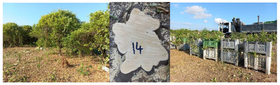
Figure 1.
Measuring, cutting down, and weighing process of tress.
To determine the fraction of leaf biomass and the fraction of woody biomass that make up the residues of the trees that were cut down, eight trees were sampled, initially measuring their weight with leaves and later their weight without leaves. The percentage of woody biomass (% Bl) was calculated by Equation (1), and the percentage of leaf biomass (% Bf) by Equation (2), where mt is the biomass of the aerial part of the whole tree, ml is the biomass of the tree without leaves.
The UNE EN 14774-3 standard was applied to determine the moisture content of the woody biomass and leaf biomass. A total of 15 wood samples and 15 leaf samples were taken when the trees were cut down, applying Equation (3), where ω is the percentage of moisture on a wet basis, mh is the weight of the initial sample, and ms is the weight of the sample after drying in an oven at 105 °C for 4 h. Wood samples had dimensions of less than 5 cm in all directions. Wet leaf samples were at least 250 g.
After weighing the tree, the dry weight of its woody biomass was calculated using Equation (4), where m is the mass of the sample, and ωl is the percentage of moisture in the woody fraction.
The dry weight of woody biomass was related to the variables related to tree geometry: trunk diameter at 10 cm from the ground (Dt), trunk perimeter at 10 cm from the ground (Pm), mean crown diameter (Dc), crown canopy height (Hc), maximum crown height (Hmax), and the sum of the diameters of the main branches.
Values from 20 samples were used to obtain predictive models of tree biomass. Subsequently, the models were validated with values from 17 different samples.
2.3. Biomass Characterization
For biomass characterization, branches with diameters in 6 ranges (0–1, 1–2, 2–3, 3–4, 4–5, and >5 cm) were selected. Five samples were taken from each diameter class for a total of 30 samples. Sample preparation followed the principles defined in the UNE-EN 14780 standard: “Solid biofuels. Sample preparation”. The main purpose of sample preparation is to reduce a sample to one or more test portions, generally smaller than the original one, without modifying its composition during each preparation stage. For this purpose, a mechanical saw and a stainless-steel hammer mill equipped with a 3 mm sieve were used.
Subsequently, the leaves were separated from each branch. These leaves were crushed with the hammer crusher and stored in airtight jars with identification labels. As the nominal particle size was less than 3 mm, the minimum mass to be retained was between 50 and 100 g.
The calorific value was obtained using a LECO® AC500 model isoperibol calorimeter, following the UNE-EN 14918 standard.
For the determination of C, H and N content, the UNE-EN ISO 16948 standard was followed. The apparatus used was the LECO® TruSpec CHN elemental analyzer. To determine the S and Cl content, the complementary module of the TruSpec CHN elemental analyzer was used to measure sulfur, in this case, following the UNE-EN 16994 standard.
For the proximate analysis of the biomass, standard muffle tests were performed according to the EN 14775: 2009 standard for ash content and EN 15148: 2009 standard for volatile matter content.
3. Results and Discussion
3.1. Analysis of Tree Geometry
Table 1 shows the statistical summary for each of the geometric variables of the trees measured. Of particular interest here is the standardized skewness and standardized kurtosis, which can be used to determine whether the sample comes from a normal distribution. Values in these statistics that fall outside the range −2 to +2 would indicate significant deviations from normality, which would tend to invalidate many of the statistical procedures usually applied to these data. In this case, none of the variables show values of standardized skewness and standardized kurtosis outside the expected range. Therefore, it is concluded that they follow a normal distribution.

Table 1.
Dendrometric variables studied.
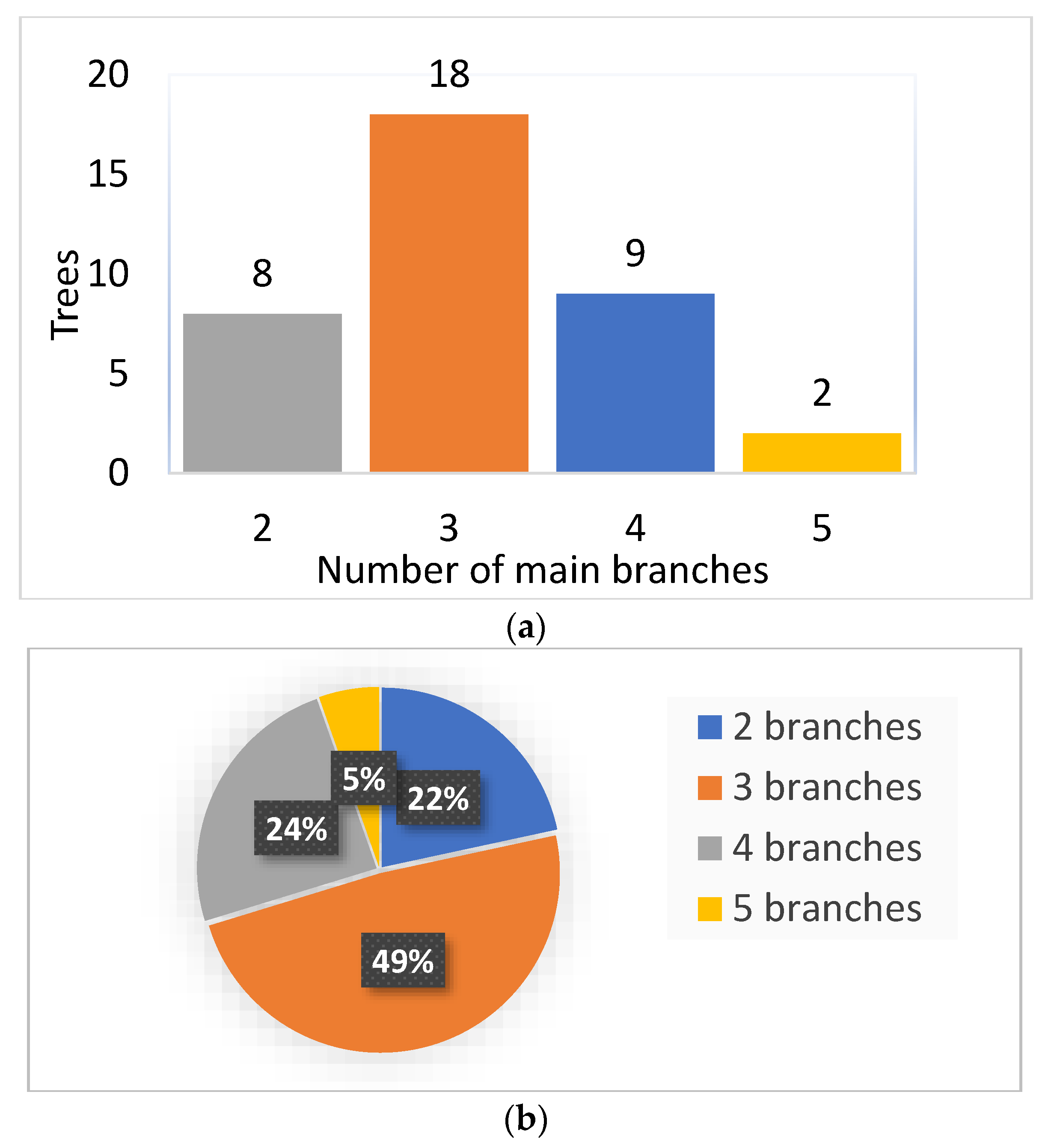
Figure 2 shows the distribution and classification of the trees according to the number of main branches, which could influence the existing aerial biomass, mainly in the crown. It can be observed that 49% of the trees evaluated have 3 main branches, 22% have 2 main branches; another 24% have 4 branches; and only 5% have 5 main branches. We believe that these frequencies of the crown structure are generally repeated in citrus trees in the study area.

Figure 2.
Frequency of trees with different numbers of main branches. (a) Absolute frequency; (b) Relative frequency.
Table 2 shows the statistical description of the woody and foliar fractions, as well as their moisture content. It can be observed that the percentage of foliar biomass in wet conditions is 13.72% of the total in the mixture, with an average moisture content of 54.15%.
Table 2.
Woody and foliar fraction and humidity.
Table 3 shows the statistical description of woody, leaf, and total biomass in the evaluated trees. It can be observed that the average wet mass of the aerial part of the tree after cutting is 113.19 kg. However, there are samples of more than 200 kg. This is especially important if the biomass is to be transported to a processing plant without pre-drying. The average dry woody biomass obtained per tree is 50.92 kg, which presents an indication of the available energy resource if destined for use as solid biofuel.
Table 3.
Statistical description of woody and foliar biomass weighted wet and dried.
To verify if the number of main branches in the tree influences the diameter of the branches or the aerial woody biomass of the tree, two analyses of variance were carried out, shown in Table 4. "a", "b" and "ab" show the similarity or significant difference between the groups. It is observed that there are no significant differences in the diameter of the branches in trees with different numbers of main branches. However, it is observed that although there is a greater number of branches, and the aerial biomass of the tree increases, there are only significant differences between trees with 2 or 3 main branches and those with 5.
Table 4.
Analysis of variance to analyze the influence of the number of branches. "a", "b" and "ab" show the similarity or significant difference between the groups.
3.2. Woody Biomass Forecasting Models
To evaluate the relationship between geometric variables and dry woody and leaf biomass, Pearson’s correlation coefficient was calculated among all measured variables. Table 5 shows the correlations between each pair of variables. These correlation coefficients range from −1 to +1 and measure the strength of the linear relationship between the variables. Variables with a significant linear p-value relationship with a confidence level greater than 95.0% are indicated with an asterisk. It can be seen that the geometric variables have very strong linear relationships with each other. Note that the only variable that does not maintain a significant relationship with aerial mass is the canopy height.
Table 5.
Correlation matrix of the measured variables.
Table 6 compares different predictive models of dry woody biomass based on their coefficient of determination r2, adjusted coefficient of determination raj2, mean absolute error (MAE), mean square error (MSE), Akaike information criterion (AIC), and Bayesian information criteria (BIC).
Table 6.
Models with Larger Adjusted r-Squared.
The adjusted r-squared statistic (raj2) measures the proportion of the variability of dry woody weight that is explained by the model where the influence of the number of variables used has been removed. The AIC value based on the residual mean square error with a penalty that increases with the number of coefficients in the model is also used. The goal is to select a model with the minimum residual error and as few coefficients as possible. The best model is the one that minimizes the AIC and MSE.
Up to five models are shown for each subset of between one and five variables. The variables are shown as A = mean trunk diameter, B = mean crown diameter, C = maximum height, D = canopy height, E = trunk circumference at 10 cm, and F = the sum of main branch diameters.
Note that the simplest model with the best r2 takes the mean diameter of the trunk at 10 cm from the ground as the explanatory variable. Its r2, at 0.68. We have used this variable for testing in polynomial models and detected that with a third-degree polynomial model, the raj2 improves significantly at 0.72, and the r2 at 0.75.
These models are beneficial because they use only one variable, and it is easier to measure in order to predict the biomass from Earth. However, if predictions are to be made from satellite or drone spectral images, the most convenient variable is crown diameter, but this variable is the worst explainer of dry woody biomass when used linearly. In addition, when polynomial models are tested, the model evaluation statistics do not improve. Table 7 compares different polynomial models based on their coefficient of determination r2, adjusted coefficient of determination raj2, MAE, root mean square (RMS), AIC, and BIC. For this reason, the use of two variables—crown diameter and tree height—is recommended for biomass analysis using Lidar or multispectral images. A linear combination of these variables gives an r2 of 0.72, but if quadratic models are used, this statistic improves to 0.78.
Table 7.
Predictive models of citrus dry woody biomass.
All the models in Table 7 have been validated.
3.3. Biomass Characterization
Table 8 shows the most important statistical values of the biomass properties of citrus trees from an energy perspective. These values allow us to balance energy, emissions, and carbon sequestration. The values are consistent with those obtained by other authors on similar types of wood, such as Velázquez et al. [16].
Table 8.
Characterization of citrus dry woody biomass.
Table 9 shows that the higher calorific value (PC, in kJ/kg) correlates well with the percentage of carbon. This is in agreement with what was reported by Callejón Ferre et al. [17].
Table 9.
Ratio of calorific value to carbon percentage.
3.4. Discussion
Two of the few existing works focused on the development of predictive models of biomass in citrus trees are Velazquez et al. [18] and Sahoo et al. [6]. The models we present in this paper have better accuracies than those reported by these authors. The models presented by Velazquez et al. [18] had lower coefficients of determination. The reason may be due to the fact that in this work, tree biomass had been measured by non-destructive methods. Velázquez et al. [18] present a system of biomass quantification by measuring the diameters and lengths of branches in different strata. This method is very laborious and can present difficulties, especially in the determination of biomass in the final layers, where the branches are small. However, in our work, the biomass values of the trees were obtained by the cutting of the trees and subsequent weighing. This system, for scientific purposes, significantly reduces the dispersion of the obtained results.
Sahoo et al. [6] presented the relationships of tree height (H) and diameter at breast height (1.3 m) (D) with aerial biomass (Y). The methods used were algorithmic:
The r2 values were between 0.61 and 0.78. These results are very similar to those obtained in our study, but the models have a drawback. The trees grown in Spain have very small trunks, making it impossible to measure their diameter at a height of 1.3 m.
Using these models, Sahoo et al. [6] indicated that the total and accumulated biomass carbon in the soil could be estimated at 7.69 and 100.2 t C/ha, respectively, in plantations in India. These values were referenced to planting densities of between 1460 and 3210 trees/ha, with an average of 2360 trees/ha in India.
According to our analysis, in plantations in the Valencia Community (Spain), where the average plantation pattern is 4 × 4 m, that is, the number of trees per hectare is significantly lower. The amount of biomass contained in one hectare is estimated at 31.82 t/ha. The amount of carbon stored in a plot is 13 t of C per hectare. As can be observed, this value is significantly higher than that reported by Sahoo et al. [6] for the aerial part, although the density of trees in Spain is lower.
The energy density in citrus can be estimated at 900 MJ/tree if leaves and wood are counted. However, if only wood is included in the calculation, the accumulated energy per tree is 750.3 MJ/tree, which represents 5.6 × 10⁵ MJ/ha.
4. Conclusions
The models developed in the present study can be applied to the estimation of stand biomass, energy, and carbon at local and regional scales in citrus orchards. However, the biomass models must first be validated before they are applied in new areas. Nevertheless, the results of the present study represent a tool with enormous potential for the accurate estimation of biomass production and carbon storage in orange orchards with more advanced remote sensing-based technologies, such as Lidar and multispectral imaging.
In addition, these tools can also be used to estimate production inputs such as water, fertilizers, or pesticides.
We suggest future studies to develop baseline data on the potential carbon credits that could be generated from these sweet-orange orchards and fruit species in all parts of the world, allowing for more precise policies to help mitigate carbon emission targets under the Kyoto Protocol (Section 3.4).
Author Contributions
Conceptualization, B.V.M. and J.E.; methodology, J.M.-G.; software, J.E. and J.M.-G.; validation, J.E.F.R.; formal analysis, I.L.-C.; investigation, I.L.-C., B.V.M., J.E., J.E.F.R., J.M.-G. and D.S.H.; resources, J.E.; data curation, J.E.F.R. and D.S.H.; writing—original draft preparation, B.V.M.; writing B.V.M.; visualization, B.V.M.; supervision, B.V.M. project administration, J.E. and B.V.M.; funding acquisition, J.E., I.L.-C. and D.S.H. All authors have read and agreed to the published version of the manuscript.
Funding
This work was funded by Gerneralitat Valenciana (Spain) through a research project (AICO/2020/246).
Institutional Review Board Statement
Not applicable.
Informed Consent Statement
Not applicable.
Data Availability Statement
All the data are available in the manuscript.
Acknowledgments
The authors wish to thank the support ofGerneralitat Valenciana (Spain) for research project (AICO/2020/246), and he IBEROMASA Network (Re 719RT0586) of the Ibero-American Program of Science and Technology for Development (CYTED) where this project has been carried out.
Conflicts of Interest
The authors declare no conflict of interest.
References
- Kuyah, S.; Dietz, J.; Muthuri, C.; Jamnadass, R.; Mwangi, P.; Coe, R.; Neufeldt, H. Allometric Equations for Estimating Biomass in Agricultural Landscapes: I. Aboveground Biomass. Agric. Ecosyst. Environ. 2012, 158, 216–224. [Google Scholar] [CrossRef]
- Velázquez-Martí, B.; Fernández-González, E.; López-Cortés, I.; Callejón-Ferre, A.J. Prediction and Evaluation of Biomass Obtained from Citrus Trees Pruning. J. Food Agric. Environ. 2013, 11, 1485–1494. [Google Scholar]
- Iglesias, D.J.; Quiñones, A.; Font, A.; Martínez-Alcántara, B.; Forner-Giner, M.Á.; Legaz, F.; Primo-Millo, E. Carbon Balance of Citrus Plantations in Eastern Spain. Agric. Ecosyst. Environ. 2013, 171, 103–111. [Google Scholar] [CrossRef]
- Yasin, G.; Farrakh Nawaz, M.; Zubair, M.; Qadir, I.; Saleem, A.R.; Ijaz, M.; Gul, S.; Amjad Bashir, M.; Rehim, A.; Rahman, S.U.; et al. Assessing the Contribution of Citrus Orchards in Climate Change Mitigation through Carbon Sequestration in Sargodha District, Pakistan. Sustainability 2021, 13, 12412. [Google Scholar] [CrossRef]
- Huang, T.-B.; Darnell, R.L.; Koch, K.E. Water and Carbon Budgets of Developing Citrus Fruit. J. Am. Soc. Hortic. Sci. Jashs 1992, 117, 287–293. [Google Scholar] [CrossRef] [Green Version]
- Sahoo, U.K.; Nath, A.J.; Lalnunpuii, K. Biomass Estimation Models, Biomass Storage and Ecosystem Carbon Stock in Sweet Orange Orchards: Implications for Land Use Management. Acta Ecol. Sin. 2021, 41, 57–63. [Google Scholar] [CrossRef]
- Bwalya, J.M. Estimation of Net Carbon Sequestration Potential of Citrus under Different Management Systems Using the Life Cycle Approach. Ph.D. Thesis, University of Zambia, Lusaka, Zambia, 2012. [Google Scholar]
- Krooks, A.; Kaasalainen, S.; Kankare, V.; Joensuu, M.; Raumonen, P.; Kaasalainen, M. Predicting Tree Structure from Tree Height Using Terrestrial Laser Scanning and Quantitative Structure Models. Silva Fenn. 2014, 48, 1125. [Google Scholar] [CrossRef] [Green Version]
- Colaço, A.F.; Molin, J.P.; Rosell-Polo, J.R.; Escolà, A. Application of Light Detection and Ranging and Ultrasonic Sensors to High-Throughput Phenotyping and Precision Horticulture: Current Status and Challenges. Hortic. Res. 2018, 5, 35. [Google Scholar] [CrossRef] [PubMed] [Green Version]
- Jiang, M.; Nakano, S. Application of Image Analysis for Algal Biomass Quantification: A Low-Cost and Non-Destructive Method Based on HSI Color Space. J. Appl. Phycol. 2021, 33, 3709–3717. [Google Scholar] [CrossRef]
- Cañada, J.; Pinazo, J.M.; Boscá, J. V Analysis of Weather Data Measured in Valencia during the Years 1989, 1990, 1991 and 1992. Renew. Energy 1997, 11, 211–222. [Google Scholar] [CrossRef]
- Vicente-Serrano, S.M.; González-Hidalgo, J.C.; de Luis, M.; Raventós, J. Drought Patterns in the Mediterranean Area: The Valencia Region (Eastern Spain). Clim. Res. 2004, 26, 5–15. [Google Scholar] [CrossRef] [Green Version]
- Gomez, I.; Estrela, M.J.; Caselles, V. Verification of the RAMS-Based Operational Weather Forecast System in the Valencia Region: A Seasonal Comparison. Nat. Hazards 2015, 75, 1941–1958. [Google Scholar] [CrossRef]
- Generalitat Valenciana Superficies y Producciones de La Comunitat Valenciana (Principales Cultivos). Available online: https://agroambient.gva.es/es/estadistiques-agricoles (accessed on 27 June 2022).
- Gregoriou, C.; Economides, C.V. Tree Growth, Yield, and Fruit Quality of Ortanique Tangor on Eleven Rootstocks in Cyprus. J. Am. Soc. Hortic. Sci. Jashs 1993, 118, 335–338. [Google Scholar] [CrossRef] [Green Version]
- Velázquez-Martí, B.; Fernández-González, E.; López-Cortés, I.; Salazar-Hernández, D.M. Quantification of the Residual Biomass Obtained from Pruning of Trees in Mediterranean Almond Groves. Renew. Energy 2011, 36, 621–626. [Google Scholar] [CrossRef]
- Callejón-Ferre, A.J.; Velázquez-Martí, B.; López-Martínez, J.A.; Manzano-Agugliaro, F. Greenhouse Crop Residues: Energy Potential and Models for the Prediction of Their Higher Heating Value. Renew. Sustain. Energy Rev. 2011, 15, 3208–3217. [Google Scholar] [CrossRef]
- Velázquez-Martí, B.; Estornell, J.; López-Cortés, I.; Martí-Gavilá, J. Calculation of Biomass Volume of Citrus Trees from an Adapted Dendrometry. Biosyst. Eng. 2012, 112, 285–292. [Google Scholar] [CrossRef] [Green Version]

Publisher’s Note: MDPI stays neutral with regard to jurisdictional claims in published maps and institutional affiliations. |
© 2022 by the authors. Licensee MDPI, Basel, Switzerland. This article is an open access article distributed under the terms and conditions of the Creative Commons Attribution (CC BY) license (https://creativecommons.org/licenses/by/4.0/).