Abstract
Off-target drift of crop protection materials from aerial spraying can be detrimental to sensitive crops, beneficial insects, and the environment. So, it is very important to accurately characterize weather effects for accurate recommendations on drift mitigation. Wind is the single-most important weather factor influencing localized off-target drift of crop protection materials. In drift sampling experiments, it is difficult to accurately characterize wind speed and direction at a drift sampling location, owing to the natural variability of spray movement on the way to the sampling target. Although it is difficult or impossible to exactly track wind movement to a target, much information can be gained by altering the way wind speed and tracking is characterized from field experiments and analyzed using statistical models of spray drift. In this study two methods of characterizing weather were compared to see how they affect results from a statistical model of downwind spray drift using field data. Use of a method that implemented weather averages over the length of a spray run resulted in model-based estimates for spray tracer concentration that compared well with field data averages. Model results using this method showed only a slight sensitivity to changes in wind speed, and this difference was more pronounced further downwind. The degree of this effect was consistent with field results. Another method that used single weather values obtained at the beginning of each run resulted in an unexpected inverse relationship of residue concentration with respect to increases in wind speed by sensitivity analysis and would thus not be recommended for use in a statistical model of downwind spray drift. This study could provide a guideline for general agricultural aviation analysis and unmanned aerial vehicle spray application studies.
1. Introduction
Modern agriculture has seen significant innovation led by precision and site-specific crop management since the late 1980s, primarily based on improvements in agricultural mechanization that integrates information from global positioning systems (GPS), remote sensing, and geographic information systems (GIS). Spatial detection methods can now better characterize within-field variability of soils, nutrients, weed and insect pests, disease, and yield. With the advancement of information and electronics technologies integrated with artificial intelligence, automation and big data, precision agriculture is moving forward to the next stage: smart agriculture [1]. In smart agriculture, agricultural production and management advances to a new level supported by supercomputing, inter-networking, machine or artificial intelligence, automation, and massive data resources in integrated fashion to optimize crop production systems and resources.
Advanced technologies have been developed for spraying systems that target pests precisely, thereby saving on pesticide costs with commensurate reduction in environmental pressure. Even so, aerial spraying systems have not caught up with ground-based spraying systems in their effectiveness for targeted spraying. By their nature, the best one can hope for is to limit spray application only to patches or small field areas. Advanced methods are still required to mitigate off target spray drift, no matter which advanced technologies are employed for site specific application.
Agricultural aviation began in 1906 by John Chaytor, who spread seed over a swamped valley floor in Wairoa, New Zealand, using a hot air balloon with mobile tethers [2]. In 1924, the first commercial operation of crop dusting was conducted in Macon, Georgia, USA, by a company named Huff-Daland Crop Dusting, co-founded by a pilot Lt. Harold R. Harris, who tested the system in McCook Field, Dayton, Ohio, USA [3]. Presently, aerial application is used in the US for plant protection and is especially useful for covering large and remote areas or where wet weather conditions preclude timely use of ground sprayers, primarily across the Midwest and Midsouth US. This makes aerial application an indispensable tool for ensuring high yields [4]. The National Agricultural Aviation Association (NAAA) (Alexandria, Virginia, USA) defines this as an industry that “consists of small businesses and pilots that use aircraft to aid farmers in producing a safe, affordable and abundant supply of food, fiber and biofuel” while “aerial application is a critical component of high-yield agriculture” (https://www.agaviation.org/aboutagaviation (accessed on 5 January 2023)).
There are some limits or challenges in aerial application of plant protection materials. Off-target drift is one of them, which may cause economic loss and environmental damage. So, in the past two decades scientists and engineers have investigated the factors and impact of off-target spray drift in plant protection. For example, in the Mississippi Delta USDA (United States Department of Agriculture), scientists have evaluated various nozzles for drift control and tested a hydraulic pump with automatic flow controller for aerial variable-rate spray studies [5]. The authors also collected meteorological data and studied the daily change and probability of atmospheric stability for the likelihood of surface temperature inversions [6,7,8]. Using these data, an algorithm was developed for a website, published to guide aerial applicators on the timing to conduct spray application for avoidance of off-target movement of spray parcels caused by temperature inversions [9,10].
Minimization of off-target drift from aerial- or ground- based spray systems [11] is critical to reduce damage to off targeted crops and to mitigate environmental effects [12]. Drift minimization practices can also work to increase application efficiency. Methods to mitigate off target movement of aerially applied agricultural materials have been well documented [13,14,15,16,17,18,19,20,21,22]. Some research efforts focus on the prediction of drift [23,24,25] from aerial spraying with several standards having been established [26,27]. Others are based on optimized drift modeling from design of experiments [28,29].
Experimental assessment of off-target drift of crop protection materials continues to be a challenge due in large part to highly variable environmental conditions. In their review of spray drift assessment methods, Felsot et al. [30] outlined two spray drift situations: the first is characterized as localized movement of agrochemical residues from target to non-target sites. In this aspect, the in-swath spray deposition of a low-drift nozzle was determined on the booms of Air Tractor 402B agricultural aircraft (Air Tractor Inc., Olney, TX, USA) [28]. Further, the spray deposition and drift from the low drift nozzle were characterized for aerial spray application of different application altitudes [31]. Using airborne remote sensing the cotton injury was assessed by spray drift from aerially applied glyphosate by spray deposition and drift sampling and measurement [32]. The second involves concentration of residues within air masses under stable atmospheric conditions. For the latter case, this mass of air with entrained chemical can drift long distances. In this aspect, Fritz et al. monitored and documented atmospheric conditions over a six-month period at two locations in Texas [22]. The measured meteorological data was used to relate low-level temperature inversion with respect to time of day, duration, and other associated meteorological conditions. Thomson et al. collected data to quantify atmospheric stability throughout the day and showed consistent patterns of atmospheric stability occurring primarily between the hours of 18:00 p.m. and 06:00 a.m. during summer months on clear days at the Mississippi Delta latitudes [6,7]. Further, results verified correctness of the three-degree rule in Arkansas when spraying on clear days in the summer months. Huang et al. determined atmospheric stability at different time intervals for determination of aerial application timing to avoid the drift caused by temperature inversion [8].
Many controlled studies have used wind tunnels to assess the droplet spectra and thus suitability of nozzles and spray mixtures for aerial and ground application [33,34]. Gil et al. developed a test bench that could examine effects of wind to complement drift quantification methods in the field or laboratory [35]. The aim was to provide a simple field method near a ground sprayer to obtain meaningful near-field drift data as a function of weather conditions. In their study, it was found that drift potential was not significantly influenced when trials were conducted at average wind velocities less than 1 m/s. Wind speed and direction greatly influenced spatial distribution of spray sample recovered along the length of the test bench.
For field studies on localized spray drift, wind speed and direction have been documented to be primary factors in downwind spray drift of crop protection materials, along with height of application when using both aerial [28,31] and ground spray platforms [36]. Fritz et al. also indicated through field experiments that wind speed was the dominant meteorological factor in transport of aerially applied sprays [37]. Wind effects have been incorporated into simulations of downwind spray drift [24], which have been verified for accuracy through field trials [24,38,39,40].
Owing to the difficulty in properly characterizing wind in drift studies, the study presented herein compares two statistical methods for acquiring weather data to observe their effect on statistically modeled downwind concentration of aerially applied spray tracer. A sensitivity analysis on selected variables, including wind speed, was performed so that their effects on modeled concentration could further be compared using both weather acquisition methods.
2. Materials and Methods
2.1. Field Experiment
Spray tests were conducted over a 15-ha open field planted in Bermuda grass at the USDA ARS, Stoneville MS, with downwind drift samplers placed at 100, 135, 200, and 320 m. Water mixed with Syl-Tac® adjuvant at standard mix of 0.25% v/v was sprayed rate of 18.7 L/ha from an Air Tractor 402B aircraft (Air Tractor, Olney, TX, USA) through 56 CP-09 straight stream (SS) nozzles (Transland LLC, Wichita Falls, TX, USA) at a release height of 3.7 m, following the same procedures as indicated by Thomson et al. [5]. Rubidium Chloride (RbCl) tracer was mixed in the tank and sampled and collected on mylar sheets and used for analyzing spray swath patterns and off-target drift. To assure consistent height of application, height of each pass was recorded using a Lasertech ULS laser (Laser Technologies, Inc., Centennial, CO, USA). The CP-09 SS nozzles were set at a 30-degree angle and operating pressure was 303 kPa corresponding to an approximate per-nozzle flow rate of 2.4 L/min. Swath width was 18.3 m and aircraft speed was 56 m/s. Nozzle parameters were set to closely match spray characteristics for a TeeJet® D6-46 hollow cone tip [41]. Volume Median Diameter (VMD) (where half of the volume of spray contains droplets larger than the VMD) was modeled to be 218 µm using the USDA ARS AATRU models [42]. This droplet size indicates a large percentage of small droplets, and the experiment was purposely set up to induce drift at long downwind distances. At this VMD, 41% of the spray volume indicated droplet diameter of 200 μm or less, and this is also consistent with the nozzle setup used by Thomson et al. [41].
Spray samplers were oriented on the day of the experiment so that wind direction was nearly perpendicular to the direction of aircraft travel. To collect enough sample at the specified downwind distances, four passes of the aircraft were made for each run. After each run, Mylar sheets were removed from stands (Figure 1) using clean rubber gloves and toothpicks on the side of each sampling sheet to direct Mylar into its own zip-lock bag. The samples were returned to the edge of the field and immediately placed into ice chests where they were protected from light. Runs were repeated sixteen times. In the laboratory, each sheet was shaken for 20 min within a rinse solution of 1% HNO3 (nitric acid solution), which was also used as a calibration blank on the AAnalyist 600 Atomic Absorption Spectrometer (Perkin Elmer, Waltham, MA, USA). Results obtained from the spectrometer for each sheet were determined in concentration units of ng/L.
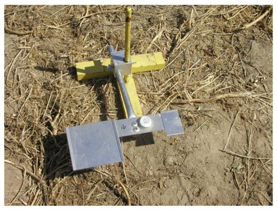
Figure 1.
Field sampling stand. Mylar sheets are held on the left bracket.
Weather data were recorded for each pass at 2-sec intervals using Kestrel 4500 weather trackers (Nielsen-Kellerman, Boothwyn, PA USA); one was set to log weather data at the beginning of each run, and one was read manually the instant spraying commenced. Using dual weather trackers facilitated testing different methods of characterizing weather effects. During the experiment, the air temperature ranged from 25 to 30 °C; relative humidity ranged from 42 to 75%; wind speed ranged from 3.3 to 5.5 m s−1. The first 4 runs were flown in an afternoon and testing continued the next day, significantly past time ranges that would indicate stable atmosphere. Wind direction was from N to NE, perpendicular to the flight-line.
Mean weather data recorded during each test run is shown in Table 1 in which all weather variables were entered into the model. Depending on how weather data were averaged for the comparisons presented herein, the actual values shown under each heading will vary. Based on air temperatures at two heights and windspeed data recorded at an adjacent tall tower [6,7], the average atmospheric stability ratio was determined as −0.36 °Cs2/m2 indicating the desirable unstable atmospheric conditions. Thus, there was no danger of entrainment of spray in an inversion layer, which would produce inaccurate results for this spray drift study.

Table 1.
Meteorological data obtained during the spray tests.
2.2. Statistical Analysis
Two methods of accounting for weather were compared. The first one averaged each of the five weather variables at the start of each pass within a single run. This method is indicated hereafter as Weather Method 1. The second method used a ten-minute average of each weather variable within which all four passes were made. This method is indicated hereafter at Weather Method 2.
PROC Mixed in SAS 9.4 provided a model-based solution for the chosen effects and tested for significance of input variables on modeled downwind residue concentration. The five weather variables and sampling distance were input to the model and the response variable was residue concentration at each sampling location. Effective distance to a sampler was adjusted for each run to account for changes in wind direction. A natural-log (ln) transform was applied to the dependent variable ‘concentration’ and downwind sampling distance. Using the ln transform gave the best model fit to actual residue data at each sampling location, as verified with SAS runs of PROC GLM. Covariance parameter estimates and non-significant variables showing little effect were progressively removed from the model as their presence influenced results. This provided robust models by which sensitivity analysis using two weather characterization methods could be achieved.
3. Results
Distance to the downwind sampler had a significant effect on the level of spray concentration at significance level of p = 0.01 for both weather methods. The solar radiation intensity was also significant at p = 0.01. Interaction of wind speed and wind direction was significant for Weather Method 1, as was the interaction of downwind distance and wind direction at significance level of p = 0.05. Weather Method 2 showed no such interaction effect of wind speed and wind direction (significance level of p = 0.8677), but also showed an interaction effect of downwind distance and wind direction at significance level of p = 0.05.
Sensitivity analysis was performed on two significant variables—wind speed and solar radiation—to see how they behaved using the two weather methods. Minimum and maximum values for these variables over duration of the experiment were used.
The effect of solar radiation on modeled downwind concentration was pronounced and comparable between the two methods, with Weather Method 2 showing a slightly greater effect. Both methods indicated a greater effect of solar radiation differences with downwind distance, as this was probably due to the longer residence time for a droplet in the air, further promoting evaporation.
Use of Weather Method 1 shows an unusual result for wind speed (Table 2). As wind speed increased, modeled sample concentration decreased markedly. Contrary to this, in-field residue data across all runs showed a weakly increasing trend in downwind concentration with increasing wind speed (Figure 2). This is trend is consistent with what had been observed in a propeller wash drift study [43]. Weather method 2 shows no such discrepancy, with an expected increase in sampled concentration with wind speed (Table 3). Values for modeled ln(concentration) were also in the range of values observed in field data across all runs. Mean ln(concentration) across all field runs was 0.331 ng/L, and this falls squarely within modeled ranges illustrated in columns 2 and 3 of Table 2. Values of modeled ln(concentration) using Weather Method 1 (Table 2) were consistently higher than this field-derived result.
Table 2.
Modeled ln (concentration) at minimum and maximum values of variables wind speed and solar radiation for Weather Method 1. Value of the other variable was held to minimum value to illustrate the effect of changes in the variable of interest.
Figure 2.
Sampled concentration of RbCl as a function of wind speed.
Table 3.
Modeled ln (concentration) at minimum and maximum values of variables wind speed and solar radiation for Weather Method 2. Value of the other variable was held to minimum value to illustrate the effect of changes in the variable of interest.
It is clear from statistical model solutions that Weather Method 2 (using weather averages over the first ten minutes of a run) yielded more reasonable results than Weather Method 1 with respect to the effect of wind speed. This points to the importance of careful characterization of weather when performing drift studies. Proper characterization may be more difficult when performing a drift study such as that described herein, that relies on several passes per run (four in this case). Although it is not immediately clear why Weather Method 2 performed better, it could be because Weather Method 1 used an average of four discrete weather events. It is very possible for wind speed and direction to change abruptly, and ten-minute weather averages (Weather Method 2) prevented discrete events from markedly influencing results. Ten minutes was the approximate time for all four passes to be completed for each run.
Statistical significance was not greatly influenced by weather characterization method, although the interaction of wind direction and wind speed was only significant at the 0.05 level for Weather Method 1. Wind speed by itself was not significant for either method, but the wind speed/wind direction interaction prompted further investigation. Wind speed results from Figure 2 (and modeled for the second weather case, (Table 3) indeed indicate only a slight effect on sampled concentration of residue.
4. Conclusions
Based on results, the following conclusions can be made regarding treatment effects on downwind sampled concentration of RbCl:
- Use of Weather Method 2, that implemented weather averages over the length of a run, resulted in model-based estimates for RbCl concentration that compared well with field data averages.
- Model results using Weather Method 2 showed only slight sensitivity to changes in wind speed, and this was more pronounced further downwind. The degree of this effect was also consistent with field results.
- The effects of changes in solar radiation were comparable between the two methods.
- Use of Weather Method 1 resulted in unexpected (inverse) relationship of RbCl concentration with respect to increases in wind speed via sensitivity analysis and would not be recommended for use in a statistical model of downwind spray drift.
- Statistically modeled downwind sampled concentration is highly sensitive to characterization of wind, and care should be taken in its measurement for realistic drift assessment.
- The experiment procedure and statistical analytical methods can be adopted for UAV spray application of plant protection materials to characterize spray deposition and off-target drift.
5. Further Discussion
The procedure and statistical methods used in this study indicating comparative drift results hold for application of plant protection materials using general agricultural aviation aircraft. Precision agriculture is now advancing to the stage of smart agriculture, which can include targeted spraying [1]. In addition to conventional manned agricultural aircraft, Unmanned Aerial Vehicles (UAVs) have been developed and adapted for targeted spray application of plant protection materials. In the future, UAVs could possibly be developed to match the tank capacities of conventional manned agricultural aircraft. UAV-based systems typically have smaller tank capacities between 10 to 60 L, and this is a more popular setting for agricultural plant protection. UAV robot swarms could be used to cover large areas.
UAV spray application began in the 1980s when crop dusting was conducted using a spray system developed on a Yamaha UAV in Japan [44]. In the US, an experiment was conducted to determine the effectiveness of using an off-the-shelf Yamaha RMAX UAV for dispersing pesticides to reduce human disease due to insects [45]. Huang et al. developed a multirotor UAV spraying system for low-volume aerial spray application [46]. Now, the technology has been developed and applied worldwide [47]. Similar to conventional aerial spray application, UAV-based spray application faces the challenge of off-target drift [48,49]. Nozzle atomization characteristics, spray deposition, and off-target drift are topics of the research to maximize spray deposition within the crop canopy and minimize off-target losses in the field and environment. For this purpose, UAV-based spraying systems need to adopt parameters from the system investigation and evaluation. The parameters include:
- Pesticide parameters—the values of the parameters depend on spray volumes, total spray amount of the system to determine spray flight operation parameter specification, coefficient of variation to measure the uniformity of the total system spray application, density of droplets, and effective swath width. Spray volumes can be high volume, medium volume, low volume, very low volume, and ultra-low volume. Among them very low (5~50 L/hm2) and ultra-low (<5 L/hm2) volumes are for UAV spray application, which can be referred to select appropriate spray nozzles.
- Flight parameters, including flight speed, flight altitude, and flight position accuracy.
- Weather parameters including air temperature, relative humidity, precipitation, wind speed, wind direction, and atmospheric stability.
Off-target drift of UAV spray application can be categorized as vapor drift and airborne drift. Vapor drift mainly occurs in the spray of herbicide such as dicamba (3, 6-dichloro-2-methoxybenzoic acid), able to control several annual and perennial broadleaf weeds. Drift of dicamba is mainly vaporized and it has deleterious effects on broadleaf plants, especially non-dicamba-tolerant (NDT) row crops. Zhang et al. assessed field NDT soybean damage from dicamba by hyperspectral remote sensing using machine learning algorithms [50].
Airborne drift occurs in the spray of herbicides such as glyphosate (primarily glyphosate [N-(phosphonomethyl) glycine) either alone or with other herbicides to manage a broad spectrum of weeds. To determine the natural downwind drift, a tracer (such as RbCl as described in this study) can be mixed in the spray solution and deposition can be determined using mylar (or other types) of spray samplers placed downwind from the spray event. Water sensitive papers can also be placed downwind or clipped to plant leaves (depending on research objectives). Droplet size and density can be calculated to determine distribution and relative quantity spray deposition. Use of water sensitive papers does not require a tracer. Droplet density or tracer concentration can be related the downwind distance to assess spray drift potential [28,31].
In addition to natural spray drift, off-target spray movement can also be exacerbated by spray application under stable atmospheric conditions. The main objective of the aircraft pilot is simply to avoid spraying under stable atmospheric conditions. Guidelines for avoidance of these conditions have been developed through research studies [6,8].
The study presented herein was an integrative investigation of parameter effects. For spray application involving single- or multi-rotor UAVs, downwash air turbulence can have a great effect on spray characteristics. Also, altitude, speed and position of a UAV are susceptible to wind disturbance. This is a much different issue than that caused by propwash effects from general aviation aircraft [42]. So, how is turbulence and wind disturbance characterized for the spray deposition and off-target drift? Results of research studies can be integrated to provide useful UAV parameter specifications for application of plant protection materials to improve efficacy and decrease off-target drift.
Author Contributions
Conceptualization, S.J.T. and Y.H.; methodology, S.J.T.; validation, S.J.T.; formal analysis, S.J.T. and Y.H.; investigation, S.J.T. and Y.H.; resources, Y.H.; data curation, S.J.T.; writing—original draft preparation, S.J.T.; writing—Y.H. All authors have read and agreed to the published version of the manuscript.
Funding
This research received no external funding.
Data Availability Statement
Data availability depends on the request with the rules and regulation of the agency with the disclaimer as “Mention of a trade name, proprietary product, or specific equipment does not constitute a guarantee or warranty by the U.S. Department of Agriculture and does not imply approval of the product to the exclusion of others that may be available”.
Conflicts of Interest
The authors declare no conflict of interest.
References
- Huang, Y.; Zhang, Q. Agricultural Cybernetics; Springer Nature: Berlin, Germany, 2021. [Google Scholar]
- Ganesh, A.S. A top-down approach. In The Hindu; Retrieved 2022-03-11; ISSN International Centre: Paris, France, 2014; ISSN 0971-751X. [Google Scholar]
- Johnson, M.A. McCook Field 1917–1927; Landfall Press: Dayton, OH, USA, 2002; pp. 190–191. [Google Scholar]
- Huang, Y. Agricultural aviation perspective on precision agriculture in the Mississippi Delta. Smart Agric. 2019, 1, 12–30. [Google Scholar]
- Thomson, S.J.; Huang, Y.; Hanks, J.E.; Martin, D.E. Improving Flow Response of a Variable-rate Aerial Application System by Interactive Refinement. Comput. Electron. Agric. 2010, 73, 99–104. [Google Scholar] [CrossRef]
- Thomson, S.J.; Huang, Y.; Fritz, B.K. Temporal indications of atmospheric stability affecting off-target spray drift in the midsouth U S. In Proceedings of the American Society of Agricultural and Biological Engineers International (ASABE); ASABE: St. Joseph, MI, USA, 2011; 8p. [Google Scholar]
- Thomson, S.J.; Huang, Y.; Fritz, B.K. Atmospheric stability intervals influencing the potential for off-target movement of spray in aerial application. Int. J. Agric. Sci. Technol. 2017, 5, 1–17. [Google Scholar] [CrossRef]
- Huang, Y.; Thomson, S.J. Atmospheric stability determination at different time intervals for determination of aerial application timing. J. Biosyst. Eng. 2016, 41, 337–341. [Google Scholar] [CrossRef]
- Huang, Y.; Fisher, D.K.; Silva, M.; Thomson, S.J. A real-time web tool for aerial application to avoid off-target movement of spray induced by stable atmospheric conditions in the Mississippi Delta. Appl. Eng. Agric. 2019, 35, 31–38. [Google Scholar] [CrossRef]
- Huang, Y.; Fisher, D.K. An open-sourced web application for aerial applicators to avoid spray drift caused by temperature inversion. Appl. Eng. Agric. 2021, 37, 77–87. [Google Scholar] [CrossRef]
- EPA (Environmental Protection Agency). Pesticide Registration (PR) Notice 2001-x Draft: Spray and Dust Drift Label Statements for Pesticide Products. Available online: https://www.epa.gov/pesticide-registration/pesticide-registration-notices-year (accessed on 20 December 2022).
- Cooper, C.D.; Alley, F.C. Air Pollution Control: A Design Approach, 2nd ed.; Waveland Press, Inc.: Prospect Heights, IL, USA, 1994. [Google Scholar]
- Yates, W.E.; Akesson, N.B.; Coutts, H.H. Evaluation of drift residues from aerial applications. Trans. ASAE 1966, 9, 389–393. [Google Scholar] [CrossRef]
- Yates, W.E.; Akesson, N.B.; Coutts, H.H. Drift hazards related to ultra-low-volume and diluted sprays applied by agricultural aircraft. Trans. ASAE 1967, 10, 628–632. [Google Scholar] [CrossRef]
- Pasquill, F.; Smith, F.B. Atmospheric Diffusion: A Study of the Dispersion of Windborne Material from Industrial and Other Sources, 3rd ed.; Ellis Horwood Limited: Chichester, UK, 1983. [Google Scholar]
- Bird, S.L. A compilation of aerial spray drift field study data for low-flight agricultural application of pesticides. In Chelsea, Mich.: Environmental Fate of Agrochemicals: A Modern Perspective; Leng, M.L., Loevey, E.M., Zubkoff, P.L., Eds.; Lewis Publishers: Chelsea, MI, USA, 1995. [Google Scholar]
- Ganzlemeier, H.; Rautmann, D.; Spangenberg, R.; Streloke, M.; Herrmann, M.; Wenzelburger, H.; Walte, H. Studies on the Spray Drift of Plant Protection Products; Blackwell Wissenschafts-Verlag GmbH: Berlin, Germany, 1995. [Google Scholar]
- Arvidsson, T. Spray Drift as Influenced by Meteorological and Technical Factors. A Methodological Study; Acta Universitatis Agriculturae Sueciae, Agraria 71; Swedish University of Agricultural Sciences: Uppsala, Sweden, 1997. [Google Scholar]
- Smith, D.B.; Bode, L.E.; Gerard, P.D. Predicting ground boom spray drift. Trans. ASAE 2000, 43, 547–553. [Google Scholar] [CrossRef]
- Hewitt, A.J.; Johnson, D.; Fish, J.D.; Hermansky, C.G.; Valcore, D.L. The development of the spray drift task force database on pesticide movements for aerial agricultural spray applications. Environ. Toxicol. Chem. 2001, 21, 648–658. [Google Scholar] [CrossRef]
- Maber, J.; Dewar, P.; Praat, J.P.; Hewitt, A.J. Real time spray drift prediction. Acta Hortic. 2001, 566, 493–498. [Google Scholar] [CrossRef]
- Fritz, B.K.; Hoffmann, W.C.; Lan, Y.; Thomson, S.J.; Huang, Y. Low-level atmospheric temperature inversions: Characteristics and impacts on aerial applications. Int. Agric. Eng. J. 2008, X, PM-08001. [Google Scholar]
- Turner, D.B. Workbook of Atmospheric Dispersion Estimates: An Introduction to Dispersion Modeling, 2nd ed.; CRC Press: Boca Raton, FL, USA, 1994. [Google Scholar]
- Teske, M.E.; Bird, S.L.; Esterly, D.M.; Curbishley, T.B.; Ray, S.L.; Perry, S.G. AgDRIFT®: A model for estimating near-field spray drift from aerial applications. Environ. Toxicol. Chem. 2002, 21, 659–671. [Google Scholar] [CrossRef] [PubMed]
- Teske, M.E.; Thistle, H.W.; Ice, G.G. Technical advances in modeling aerially applied sprays. Trans. ASAE 2003, 46, 985–996. [Google Scholar] [CrossRef]
- EPA (Environmental Protection Agency). Meteorological Monitoring Guidance for Regulatory Modeling Applications; EPA-454/R-99-005; USEPA Office of Air Quality Planning and Standards: Research Triangle Park, NC, USA, 2000. [Google Scholar]
- ASAE S561.1; Procedures for Measuring Drift Deposits from Ground, Orchard, and Aerial Sprayers. ASABE: St. Joseph, MI, USA, 2004.
- Huang, Y.; Thomson, S.J. Characterization of in-swath spray deposition for CP-11TT flat-fan nozzles used in low volume aerial application of crop production and protection materials. Trans. ASABE 2011, 54, 1973–1979. [Google Scholar] [CrossRef]
- Huang, Y.; Zhan, W.; Fritz, B.K.; Thomson, S.J. Optimizing selection of controllable variables to minimize downwind drift from aerially applied sprays. Appl. Eng. Agric. 2012, 28, 307–314. [Google Scholar] [CrossRef]
- Felsot, A.S.; Unsworth, J.B.; Linders, J.B.H.J.; Roberts, G.; Rautman, D.; Harris, C.; Carazo, E. Agrochemical spray drift; assessment and mitigation—A review. J. Environ. Sci. Health Part B Pestic. Food Contam. Agric. Wastes 2011, 46, 1–23. [Google Scholar] [CrossRef]
- Huang, Y.; Thomson, S.J. Characterization of spray deposition and drift from a low drift nozzle for aerial application at different application altitudes. Int. J. Agric. Biol. Eng. 2011, 4, 1–6. [Google Scholar]
- Huang, Y.; Thomson, S.J.; Ortiz, B.V.; Reddy, K.N.; Ding, W.; Zablotowicz, R.M.; Bright, J.R. Airborne remote sensing assessment of the damage to cotton caused by spray drift from aerially applied glyphosate through spray deposition measurements. Biosyst. Eng. 2010, 107, 212–220. [Google Scholar] [CrossRef]
- Hoffmann, W.C.; Fritz, B.K.; Thornburg, J.W.; Bagley, W.E.; Birchfield, N.B.; Ellenberger, J. Spray drift reduction evaluations of spray nozzles using a standardized testing protocol. J. ASTM Int. 2010, 7, JAI102820. [Google Scholar] [CrossRef]
- Ferguson, C.; O’Donnell, C.C.; Chauhan, B.S.; Adkins, S.W.; Kruger, G.R.; Wang, R.; Ferreira, P.H.U.; Hewitt, A.J. Determining the uniformity and consistency of droplet size across spray drift reducing nozzles in a wind tunnel. Crop Prot. 2015, 76, 1–6. [Google Scholar] [CrossRef]
- Gil, E.; Gallarta, M.; Balsari, P.; Marucco, P.; Almajanoc, M.P.; Llop, J. Influence of wind velocity and wind direction on measurements of spray drift potential of boom sprayers using drift test bench. Agric. For. Meteorol. 2015, 202, 94–101. [Google Scholar] [CrossRef]
- Fritz, B.K. Meteorological effects on deposition and drift of aerially applied sprays. Trans. ASABE 2006, 49, 1295–1301. [Google Scholar] [CrossRef]
- Arvidsson, T.; Bergstrom, L.; Kreuger, J. Spray drift as influenced by meteorological and technical factors. Pest Manag. Sci. 2009, 67, 586–598. [Google Scholar] [CrossRef] [PubMed]
- Bird, S.L.; Perry, S.G.; Ray, S.L.; Teske, M.E. Evaluation of the AgDISP aerial spray algorithms in the AgDRIFT model. Environ. Toxicol. Chem. 2002, 21, 672–681. [Google Scholar] [CrossRef]
- Woods, N.; Craig, I.P.; Dorr, G.; Young, B. Spray drift of pesticides arising from aerial application in cotton. J. Environ. Qual. 2001, 30, 697–701. [Google Scholar] [CrossRef] [PubMed]
- Thistle, H.W.; Teske, M.E.; Richardson, B.; Strand, T.M. Model physics and collection efficiency in estimates of pesticide spray drift model performance. Trans. ASABE 2020, 63, 1939–1945. [Google Scholar] [CrossRef]
- Thomson, S.J.; Womac, A.; Mulrooney, J. Reducing pesticide drift by considering propeller rotation effects from aerial application near buffer zones. Sustain. Agric. Res. 2013, 2, 41–51. [Google Scholar] [CrossRef]
- CPNozzles. Calculation Tools. Available online: https://cpnozzles.com/calculation-tools/ (accessed on 20 December 2022).
- Thomson, S.J.; Young, L.D.; Bright, J.R.; Foster, P.N.; Poythress, D.D. Effects of Spray Release Height and Nozzle/Atomizer Configuration on Penetration of Spray in a Soybean Canopy—Preliminary Results; Technical Paper AA07-008; National Agricultural Aviation Association (NAAA): Washington, DC, USA, 2007. [Google Scholar]
- Sato, A. The RMAX Helicopter UAV; Public Report; Aeronautic Operations; Yamaha Motor Co., Ltd.: Shizuoka, Japan, 2003. [Google Scholar]
- Miller, J.W. Report on the Development and Operation of an UAV for an Experiment on Unmanned Application of Pesticides; AFRL, USAF: Youngstown, OH, USA, 2005. [Google Scholar]
- Huang, Y.; Hoffmann, W.C.; Lan, Y.; Wu, W.; Fritz, B.K. Development of a spray system for an unmanned aerial vehicle platform. Appl. Eng. Agric. 2009, 25, 803–809. [Google Scholar] [CrossRef]
- Chen, P.; Douzals, J.P.; Lan, Y.; Cotteux, E.; Delpuech, X.; Pouxviel, G.; Zhan, Y. Characteristics of unmanned aerial spraying systems and related spray drift: A review. Front. Plant Sci. 2022, 13, 2726. [Google Scholar] [CrossRef]
- Wang, C.; Herbst, A.; Zeng, A.; Wongsuk, S.; Qiao, B.; Qi, P.; Bonds, J.; Overbeck, V.; Yang, Y.; Gao, W.; et al. Assessment of spray deposition, drift and mass balance from unmanned aerial vehicle sprayer using an artificial vineyard. Sci. Total Environ. 2021, 777, 146181. [Google Scholar] [CrossRef] [PubMed]
- Biglia, A.; Grella, M.; Bloise, N.; Comba, L.; Mozzanini, E.; Sopegno, A.; Pittarello, M.; Dicembrini, E.; Eloi Alcatrão, L.; Guglieri, G.; et al. UAV-spray application in vineyards: Flight modes and spray system adjustment effects on canopy deposit, coverage, and off-target losses. Sci. Total Environ. 2022, 845, 157292. [Google Scholar] [CrossRef] [PubMed]
- Zhang, J.; Huang, Y.; Reddy, K.N.; Wang, B. Assessing crop damage from dicamba on non-dicamba-tolerant soybean by hyperspectral imaging through machine learning. Pest Manag. Sci. 2019, 75, 3260–3272. [Google Scholar] [CrossRef] [PubMed]


Disclaimer/Publisher’s Note: The statements, opinions and data contained in all publications are solely those of the individual author(s) and contributor(s) and not of MDPI and/or the editor(s). MDPI and/or the editor(s) disclaim responsibility for any injury to people or property resulting from any ideas, methods, instructions or products referred to in the content. |
© 2023 by the authors. Licensee MDPI, Basel, Switzerland. This article is an open access article distributed under the terms and conditions of the Creative Commons Attribution (CC BY) license (https://creativecommons.org/licenses/by/4.0/).