Article

Canopy Laser Interception Compensation Mechanism—UAV LiDAR Precise Monitoring Method for Cotton Height

1
College of Electronic Engineering, South China Agricultural University, Guangzhou 510642, China
2
Rice Research Institute, Guangdong Academy of Agricultural Sciences, Guangzhou 510640, China
3
National Center for International Collaboration on Precision Agricultural Aviation Pesticide Spraying Technology, Guangzhou 510642, China
4
College of Agriculture, South China Agricultural University, Guangzhou 510642, China
5
Department of Biological and Agricultural Engineering, Texas A&M University, College Station, TX 77843, USA
*
Author to whom correspondence should be addressed.
These authors contributed equally to this work.
Agronomy 2023, 13(10), 2584; https://doi.org/10.3390/agronomy13102584
Submission received: 11 September 2023 / Revised: 28 September 2023 / Accepted: 3 October 2023 / Published: 9 October 2023
(This article belongs to the Special Issue New Trends in Agricultural UAV Application)

Abstract

:
Plant height is a crucial phenotypic trait that plays a vital role in predicting cotton growth and yield, as well as in estimating biomass in cotton plants. The accurate estimation of canopy height from single-flight LiDAR data remains a formidable challenge in current high-density cotton cultivation patterns, where dense foliage obstructs the collection of bare soil terrain, particularly after flowering. The existing LiDAR-based methods for cotton height estimation suffer from significant errors. In this study, a new method is proposed to compensate for the canopy height estimation by using the canopy laser interception rate. The ground points are extracted by the ground filtering algorithm, and the interception rate of the laser per unit volume of the canopy is calculated to represent the canopy density and compensate for the cotton height estimation. The appropriate segmented height compensation function is determined by grouping and step-by-step analysis of the canopy laser interception rate. Verified by 440 groups of height data measured manually in the field, the results show that the canopy laser interception compensation mechanism is of great help in improving the estimation accuracy of LiDAR. R2 and RMSE reach 0.90 and 6.18 cm, respectively. Compared with the estimation method before compensation, R2 is increased by 13.92%, and RMSE is reduced by 49.31%. And when the canopy interception rate is greater than 99%, the compensation effect is more obvious, and the RMSE is reduced by 62.49%. This research result can significantly improve the height estimation accuracy of UAV-borne for high planting density cotton areas, which is helpful to improve the efficiency of cotton quality breeding and match genomics data.

1. Introduction

Benefiting from the development of high-throughput sequencing technology, genomics research has made great progress. However, the lag in phenotype information acquisition technology has led to its inability to synchronously match data-rich genomics data, which has seriously hindered the breeding process and become a bottleneck in current cotton breeding selection research [1]. Cotton is the main raw material of the textile industry and an important cash crop. Plant height is a significant phenotypic trait of cotton that serves as a crucial predictor in yield estimation [2], biomass estimation [3], and lodging resistance [4]. Therefore, it is of great significance to obtain the height of cotton crops in a large area. Traditionally, crop heights are obtained by field measurements, which are time-consuming and labor-intensive, making it impractical to obtain heights over large areas.
Crop height monitoring based on UAV remote sensing can be mainly divided into two categories: reflection spectrum inversion and three-dimensional reconstruction measurement. Passive optical remote sensing image based on drones has been widely used in the field of crop phenotype monitoring, such as cotton’s single boll weight [5], chlorophyll content [6], leaf area index [7], etc. In addition, many studies have emerged to obtain the height of various crops (e.g., rice [8], corn [9], wheat [10], and soybean [11] by acquiring high overlap images using UAVs with visible light cameras, feature detection and matching based on structure from motion (SfM) algorithms and constructing point cloud models. However, optical remote sensing data are prone to saturation in areas of high biomass or high LAI (leaf area index) [12] and, therefore, have significant limitations in studies of predicting crop structural parameters, such as vegetation height. This phenomenon can be mitigated to some extent by fusing millimeter-wave radar data, but the overall effect remains unsatisfactory [13]. In addition, digital cameras cannot penetrate the vegetation canopy to obtain ground height data, so accurate crop height estimation generally requires two flying missions, including collecting digital terrain models (DEM) without vegetation cover during sowing and after harvest and digital surface model (DSM) data with crop cover, which greatly reduces the convenience of data acquisition. This method has a root mean square error of 8.4 cm on cotton plant height monitoring in the case of using a laser land leveling machine before sowing [14].
LiDAR is characterized by its high penetration ability, allowing it to capture the topography and characteristics of both the ground surface and target objects simultaneously via multiple laser pulse reflections. Early LiDAR is usually carried on helicopters or fixed-wing aircraft to measure forest canopy heights [15]. However, the flight altitude of airborne LiDAR usually exceeds 100 m, with limited spatial resolution, making it difficult to distinguish between soil and low crops. Terrestrial LiDAR systems are capable of acquiring three-dimensional point cloud data with millimeter-level accuracy, and there are many related studies in the direction of crop height extraction in the form of robotic platforms [16], vehicle-mounted platforms [17], and ground-based fixed platforms [18]. However, the ground-based fixed platform is less efficient in acquiring data, and the ground-based mobile platform has to take into account the information on cultivation spacing and line spacing of field crops as well as crop height, which is less suitable for land-intensive crops.
The advent of unmanned airborne LiDAR systems fills the gap between ground-based platforms with high accuracy but low efficiency and manned platforms with large scale but little detail information. LiDAR-based crop height estimation can be derived in different ways, such as the percentage method [19], canopy height model (CHM)-based method [20], and point cloud variable-based method [11]. However, in the case of extremely high canopy density, the loss of ground points will increase the error of plant height estimation, especially in the current cotton cultivation model with “low appearance, high density, and early maturity” as the mainstream [21], the planting density has reached 20 plants/m2 or more, resulting in an error of about 10 cm in cotton plant height extraction [22], causing great difficulties in matching genomics data. Therefore, it is very important to study how to improve the accuracy of LiDAR estimation of plant height under the condition of high canopy density, which will help to quickly locate the relevant genetic locus to speed up the process of variety breeding and can also provide a reference for crop protection by aircraft to formulate suitable operational parameters. Relevant studies have shown that airborne LiDAR has a good effect on cotton leaf area index inversion (R2 = 0.950, RMSE = 0.332) [23]. However, the number of studies reported in the existing literature on the use of drone LiDAR to estimate the height of cotton is very small, and the accuracy of the results is not high.
If the density of the LiDAR laser is greater than the size of the canopy gap, some of the laser beams will be obstructed by the canopy, resulting in the inability to obtain ground points. This, in turn, will lead to a high-ground grid generated through interpolation, ultimately impacting the accuracy of estimation results. The main purpose of this study is based on the fact that UAV-borne LiDAR can accurately obtain the plant height of cotton in the field through a single sortie. By extracting ground points to generate a ground grid, combined with the digital surface model obtained by a point cloud grid, the canopy laser interception rate is used to compensate for the canopy density to obtain a relatively accurate cotton height. This study aims to address the long-standing problem of insufficient precision in monitoring cotton plant height in large-scale field experiments by exploring the mapping relationship between canopy density and ground filtering errors. By bridging the gap between genotype, phenotype, and environment, this research can advance the breeding process of high-quality cotton varieties. The main contents of this study include:
(1)
Analyzing a suitable ground point filtering algorithm for the cotton point cloud model in fields;
(2)
Research on a compensation mechanism for plant height in canopy laser interception to solve the problem of laser penetration;
(3)
Improving the accuracy of canopy height models (CHM).

2. Materials and Methods

2.1. Experimental Area and Field Sampling

In this experiment, Shihezi of Xinjiang and Jiujiang of Jiangxi are selected for research, representing the typical planting patterns of cotton areas in Xinjiang and cotton areas in the Yangtze River Basin, respectively (Figure 1). Among them, the breeding experimental field in Shihezi of Xinjiang has a total of 875 different variety materials, and each community is a square with a side length of 5 m. The application rates of 15 different concentrations of nitrogen, potassium, and boron fertilizers and blank control groups are designed in the water and fertilizer experimental field located in Jiujiang of Jiangxi Province for a total of 24 communities. The huge differences in cotton growth in different regions, varieties, and cultivation modes make the conclusions of this study more convincing.
Field sampling was conducted between 6 August 2022 and 15 October 2022, and actual canopy height values in the field were measured using a tape measure (Figure 2a) and a Trimble GEO 7X GNSS handheld data collection device for centimeter-level accuracy spatial position recording (Figure 2b). Due to the impact of the COVID-19 pandemic, Shihezi City adopted epidemic containment measures on August 6, so only one data collection was carried out in Shihezi. A total of 440 field plant height measurement data were collected in the experiment, as shown in Figure 2c.
A flowchart outlining the overall methodology is presented in Figure 3. Subsequent sections describe all the steps in detail.

2.2. Point Cloud Data Collection and Preprocessing

2.2.1. Data Acquisition and Splicing of UAV Borne LiDAR

The DJI M300 RTK aircraft is used to carry out point cloud data acquisition with ZENMUSE L1 LiDAR (Figure 4). The aircraft is integrated with a differential positioning module and has a strong anti-magnetic interference capability and precise positioning capability. ZENMUSE L1 integrates the Livox LiDAR module, high-precision inertial navigation, mapping camera, three-axis PTZ, and other modules, enabling all-weather, efficient real-time three-dimensional data acquisition and high-precision post-processing and reconstruction in complex scenes.
Due to the extremely high density of the cotton canopy, in order to ensure the number of ground points in the collected point cloud data, all parameters are set to obtain the maximum point cloud density during data collection. The flight height was 12 m, the flight speed was 1 m/s, and the sampling frequency was 240 kHz. The laser point cloud overlap rate was set to 10% to ensure slicing adjustment. A double-pulse scanning mode was used to collect point cloud data, with a point cloud density of 11,000 points/m2. Specific hardware parameters are shown in Table 1.
It can be seen that after the UAV LiDAR data collection is completed, the data will be spliced through the DJI Terra software. The software will automatically read the point cloud data and inertial navigation records, track files and other related data for POS resolving, point cloud coloring, splicing, and other operations, and generate LAS point cloud files after completion.

2.2.2. Point Cloud Data Preprocessing

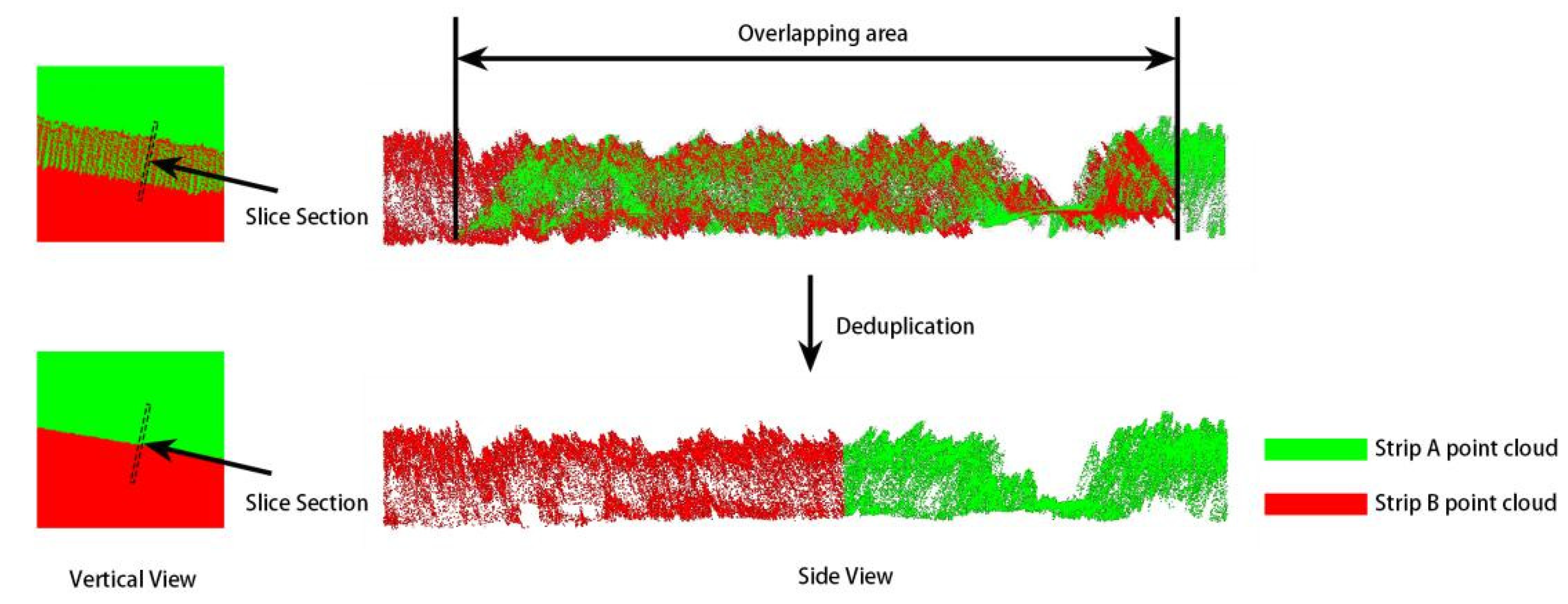
First, to avoid the influence of point cloud noise on the test results, the statistical filtering method was used to filter the original point cloud to remove high and low gross errors. The 10% overlap rate of the airstrip at the time of data acquisition leads to a significant increase of the point cloud density in the overlap area, which will affect the canopy LiDAR interception rate calculated later, so the redundant points in the overlap area need to be removed. Usually, the measurement error of LiDAR points is proportional to the laser scan angle, and the closer to the strip edge, the larger the error of the point cloud is. For the redundant part of the airborne LiDAR air strip overlap region, the redundancy removal function of LiDAR360 (Beijing Green Valley Technology. Co., Ltd., Beijing, China) software is applied, based on the complete route information, with the theoretical basis that the point cloud accuracy decreases with the increase of scan angle. In this way, the points with larger scanning angles in the overlapping area are removed, and the points with higher quality near the center of the line strip are retained so as to eliminate the redundancy of aerial photography data between the airstrips. The effect of redundancy removal is shown in Figure 5.
The preprocessing of remote sensing data is completed in the Power LeaderTM PR490P computing server. DJI Terra is used to splice the images taken by the UAV. The software will automatically read the EXIF information of the images and find the same name points in a single image to generate an orthophoto panorama of the research area.

2.3. Ground Point Extraction

By comparing and testing the performance of two ground filtering algorithms, namely Progressive Triangular Irregular Network Densification (PTD) and Gravity Cloth Filter (CSF), in a dense canopy scene, a suitable ground point filtering algorithm is selected for ground point extraction, and the ground grid is generated by Delaunay triangular network.

2.3.1. Progressive TIN Densification (PTD) Ground Filtering

Progressive Triangular Irregular Network Densification is a classic ground filtering algorithm [24], which has achieved the best results in the filtering algorithm test conducted by ISPRS (International Society for Photogrammetry and Remote Sensing). The main idea of the PTD algorithm is to construct an initial irregular triangulation network (TIN) through the initial ground seed points and then make iterative judgments on the remaining points. If the requirements are met, add the ground point set to make the TIN constructed in the next iteration more refined. The process is performed iteratively until no new ground points appear or reach the maximum number of iterations. The main steps are as follows:
(1)
Low point removal. Due to the multi-path effect of the LiDAR system or due to errors in the laser ranging system, there is a probability that laser points with much lower elevation than other points around them will be formed. If these points are not removed, then the ground seed point selection using the above assumptions will result in a set of ground seed points containing these low points, which will introduce errors in the subsequent filtering;
(2)
Ground seed point selection. Define a cube boundary box to wrap the point cloud data and divide it into n rows and m columns and multiple areas. According to the principle of the lowest local elevation, the ground seed points are evenly selected from the original point cloud, and the remaining points are the points to be judged. n and m can be obtained by Formula (1), where x and y are the length and width of the cube boundary, and bmax is set to the width of the ridge in this experiment;
n = x b max m = y b max
(3)
Construct the initial TIN. Use the initial ground seed points selected in (2) to construct the initial TIN (Figure 6);
(4)
Select the ground point from the points to be judged for iterative encryption. For all the points to be judged, find the triangular plane whose projection coordinates in the xoy plane correspond to the triangular plane in the TIN and calculate the slope of the triangular plane at the same time. If the slope is greater than the set maximum slope α1, use the mirror image point (Figure 7a) to judge. The classification of this point is consistent with the classification of the mirror point, and find the vertex Ph(xm,ym,zm) with the largest elevation value in the triangle where the point P to be judged is located. The coordinates of the P point can be calculated by Formula (2);
x m i r r o r = 2 x m x P y m i r r o r = 2 y m y P z m i r r o r = 2 z P
If the slope of the triangular surface is less than α1, calculate the distance h from the point to be judged to the triangular surface and the angle α between the line connecting the point to be judged and the vertex of the nearest triangular plane and the triangular plane. As shown in Figure 7b, if α < α1 and h is less than the set maximum height h1, the point to be judged is regarded as the ground point and counted in the ground point set. Then, rebuild the TIN and perform the above operations iteratively until no new ground points are selected, or the preset maximum number of iterations is reached.
Figure 7. (a) Mirroring process and (b) Calculation of α and h.
Agronomy 13 02584 g007

2.3.2. Cloth Simulation Filter (CSF) Ground Filtering

Cloth Simulation Filter (CSF) performs ground point filtering from a new perspective [25], and its process is to first invert the point cloud along the Z-axis and subsequently assume that a piece of fabric falls from above under the influence of gravity, then the final falling fabric can represent the current terrain, as shown in Figure 8. the CSF filtering algorithm does not need to set various complicated parameters in the filter, and the CSF filtering algorithm is stronger in ease of use than traditional ground filtering algorithms (such as PTD, etc.).
The CSF filtering algorithm assumes that the fabric particle receives gravity G during its fall as well as the internal tractive force Fin of the particle, then according to Newton’s second formula, the position X of the fabric particle at moment t satisfies.
m X t t 2 = G + F i n X , t
Then, in the case of no internal force, the displacement of the cloth particles is:
X t + Δ t = 2 X t X t Δ t + G m Δ t 2
Add an internal traction Fin to constrain the falling problem of particles in the blank area of the overturning surface. Take any two adjacent particles; if the states of both particles are movable, they move the same distance in the opposite direction; if one particle is immovable, move the movable particles in the opposite direction. The displacement of particle d can be calculated using the following formula:
d = 1 2 p a + p b n
In the formula, n is the unit vector in the vertical direction, and Pb is the adjacent particle to Pa. Figure 9 shows the movement process of the cloth particles. At the same time, the parameter RI is introduced to describe the number of times the particles move by the internal force image so as to characterize the “hardness” of the simulated cloth. Generally speaking, the steeper the terrain, the smaller the RI value is set.

2.4. Compensation of Canopy Laser Interception Rate

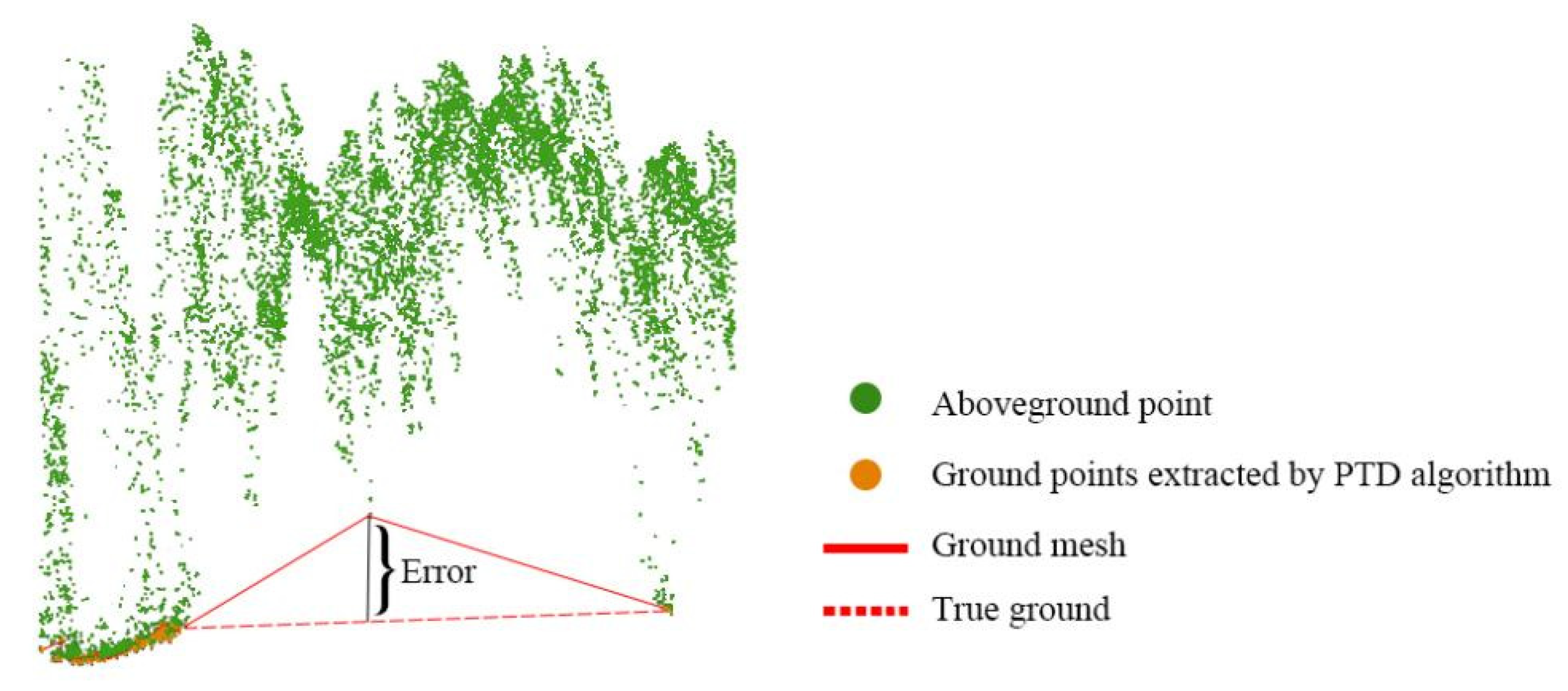
When the canopy gap is smaller than the LiDAR laser density, all the lasers will be intercepted by the canopy, and thus, the ground points will not be obtained, which will cause the ground grid generated by interpolation to be high (Figure 10) and affect the estimation results. In this study, we propose to use the canopy laser interception rate to characterize the canopy density and compensate for the estimation results to obtain more accurate estimation accuracy (Formula (6)). The HLiDAR in the formula denotes the height obtained by subtracting between the DSM and DEM generated using the point cloud, α is the compensation factor, and P denotes the canopy laser interception rate.
H = H L i D A R + f ( α ) P
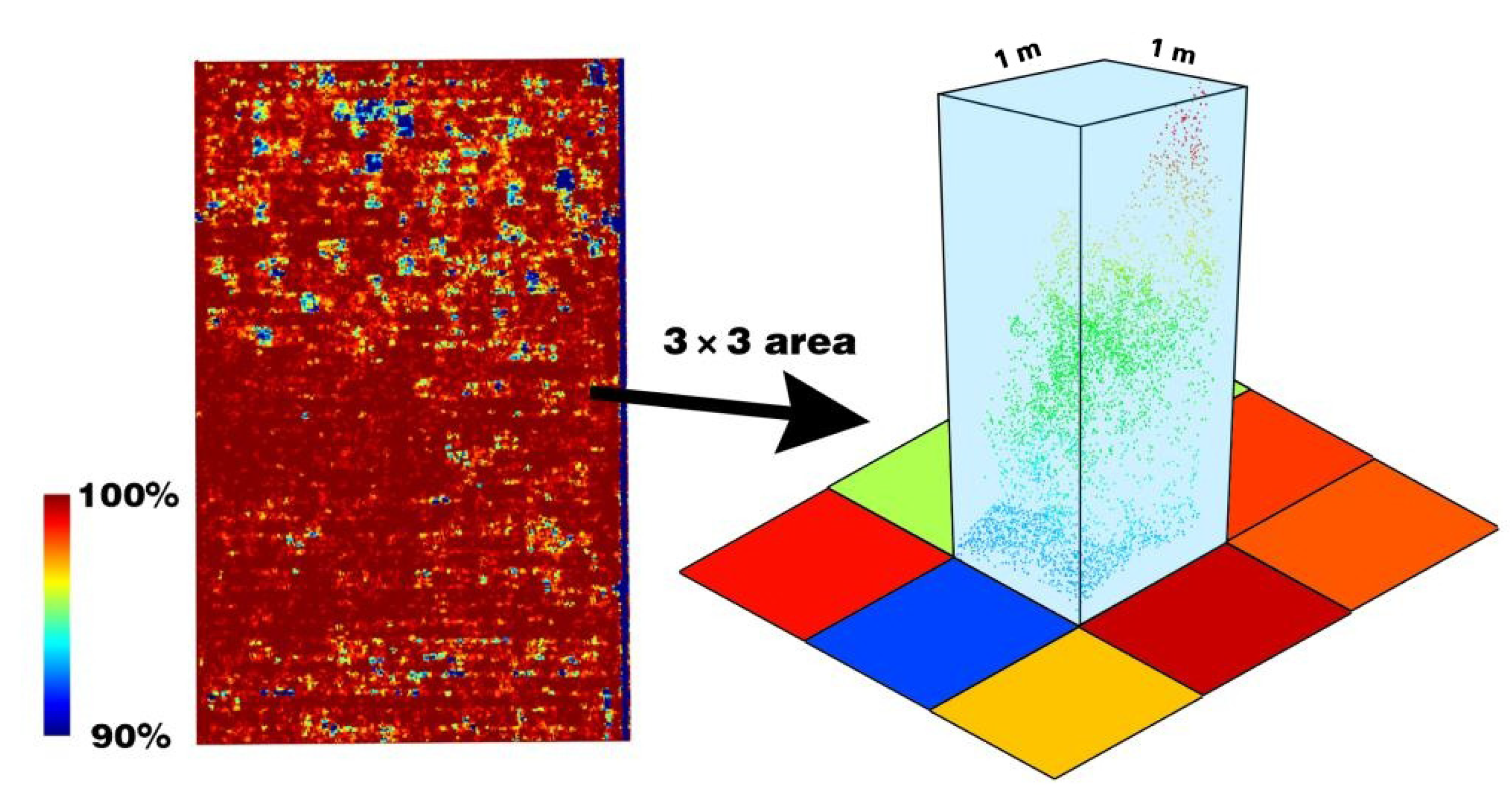
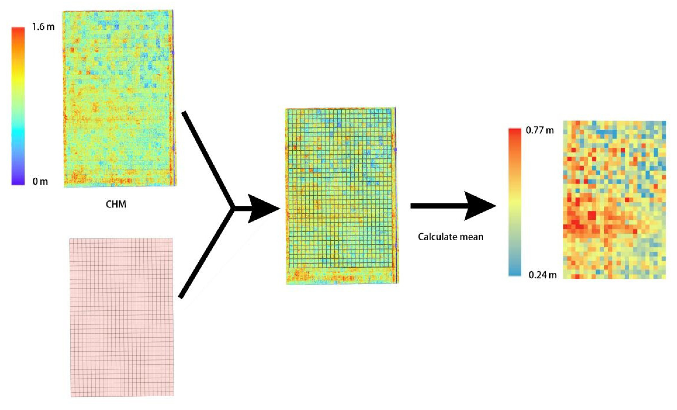
The point cloud is projected in the xoy plane, the entire area is divided into a square grid with a side length of 1 m, several areas with a side length of 1 square meter are generated, and the proportion P of non-ground points in each area is counted, and finally, the grid map of canopy laser interception rate in the study area is generated (Figure 11).

2.5. Evaluation Index

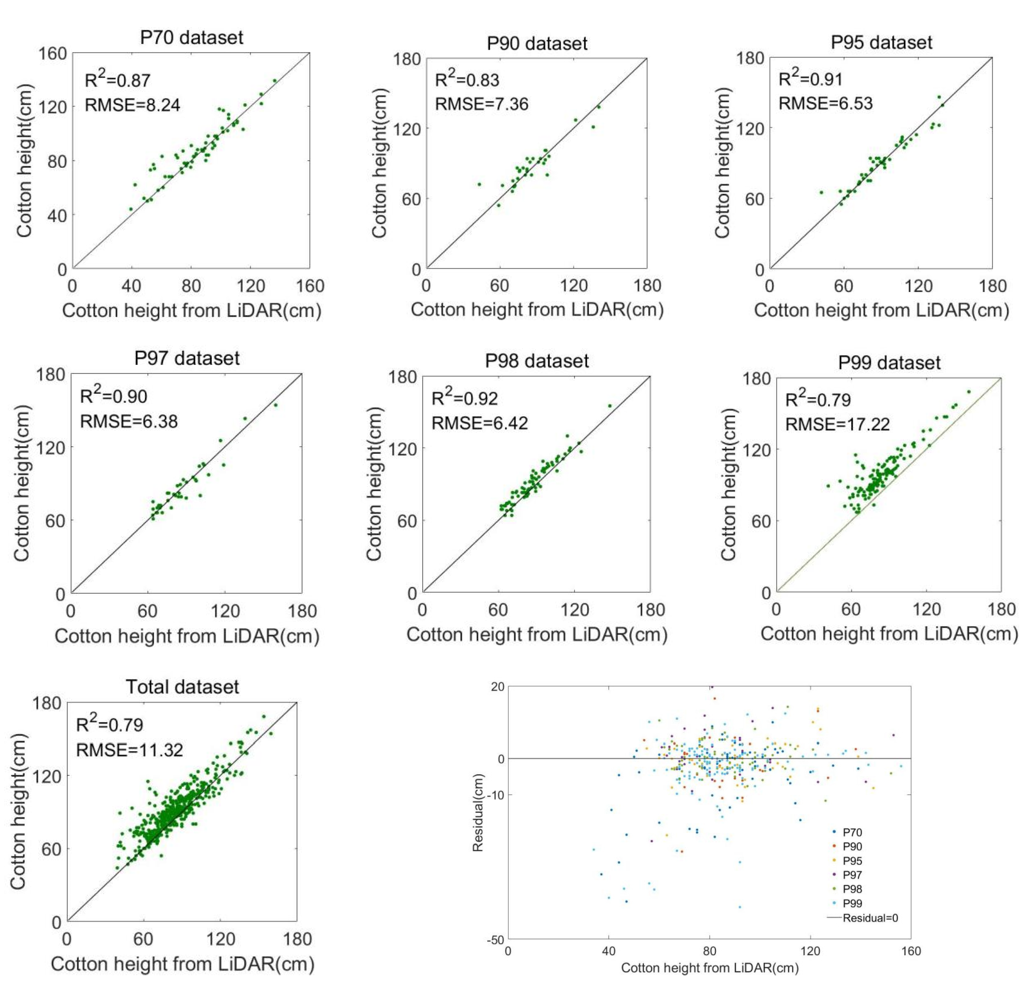
In this study, two statistical indicators, the determination coefficient R2 and the root mean square error RMSE, are used to evaluate the performance of the plant height estimation model. To investigate the impact of canopy density on the precision of LiDAR-based plant height estimation, this study produced 6 datasets—P70, P90, P95, P97, P98, and P99 from the total number of samples, respectively, representing different canopy densities. The mean and standard deviation (Std) of each dataset is shown in Table 2.

3. Results

3.1. Influence of Ground Filtering Algorithm

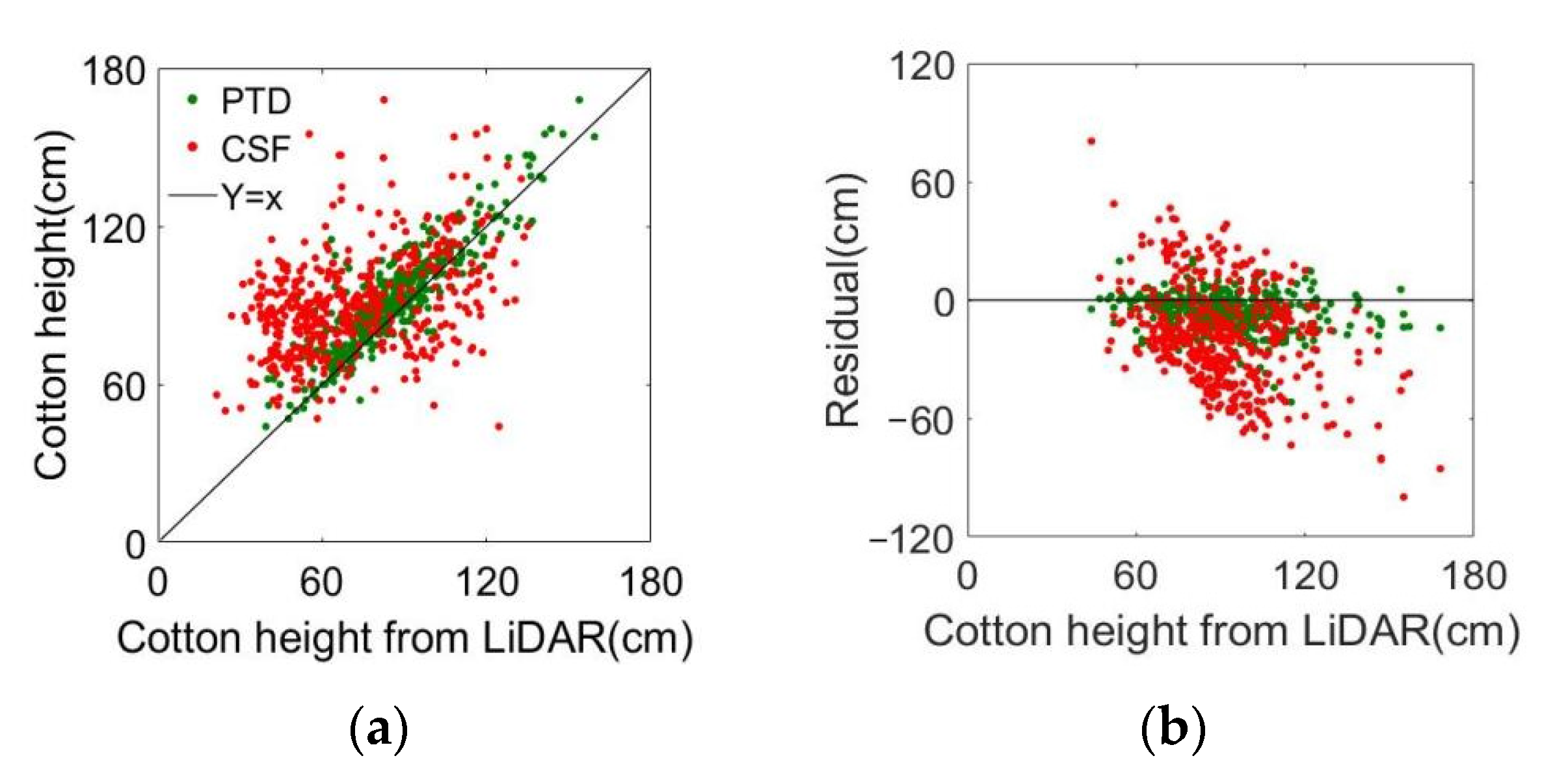
The performance of two-point cloud ground filtering algorithms, PTD and CSF, is tested on the data collected in this study. DSM and DEM are obtained by rasterizing the non-ground points and ground points, respectively, in the Z-axis direction, and CHM is obtained by subtracting them. The matching between CHM-PTD and CHM-CSF and actual ground-measured samples is shown in Figure 12.
The results show that in the high canopy density environment where this study is located, the effect of PTD (R2 = 0.79) is significantly better than that of CSF (R2 = 0.29), and it can be seen from the residual error diagram that the latter is significantly lower in estimation. From the section view (Figure 13), the difference in the ground mesh obtained by the two filtering algorithms can be clearly seen. It is preliminarily inferred that the “sharp” shape formed by the laser penetrating the canopy can easily pass through the gap between the cloth particles, resulting in the result of CSF filtering that is not the ground but the lower surface of the canopy. Therefore, the follow-up of this research will be based on the CHM taken by the PTD algorithm.

3.2. Effect of Canopy Density

Figure 14 shows the matching degree and residual error map of CHM-PTD with the six different canopy density datasets in Table 2. From the matching situation of the P99 dataset and the residual error map, it can be seen that when the canopy interception rate is greater than 99%, the estimation accuracy of LiDAR decreases sharply (R2 = 0.79, RMSE = 17.22 cm), and there is an overall smaller trend, which directly reduces the estimation accuracy of the total sample. Therefore, an f (α) compensation function is introduced to estimate and compensate for the position where the laser canopy rate is greater than 99% to make up for the low CHM phenomenon caused by the inability of the laser to penetrate the canopy.

3.3. Determination of Compensation Function f(α)

To obtain the optimal compensation coefficient under different laser canopy interception rates, add the αP formula as compensation in the estimated original plant height. Table 3 shows the estimation equation and the comparison of R2 and RMSE before and after compensation. It can be seen that the estimation accuracy of the compensation estimation method in P98, P99, and the total sample has been significantly improved, while the accuracy improvement of the compensation method in other datasets is not obvious and even has cases of negative optimization in some datasets.
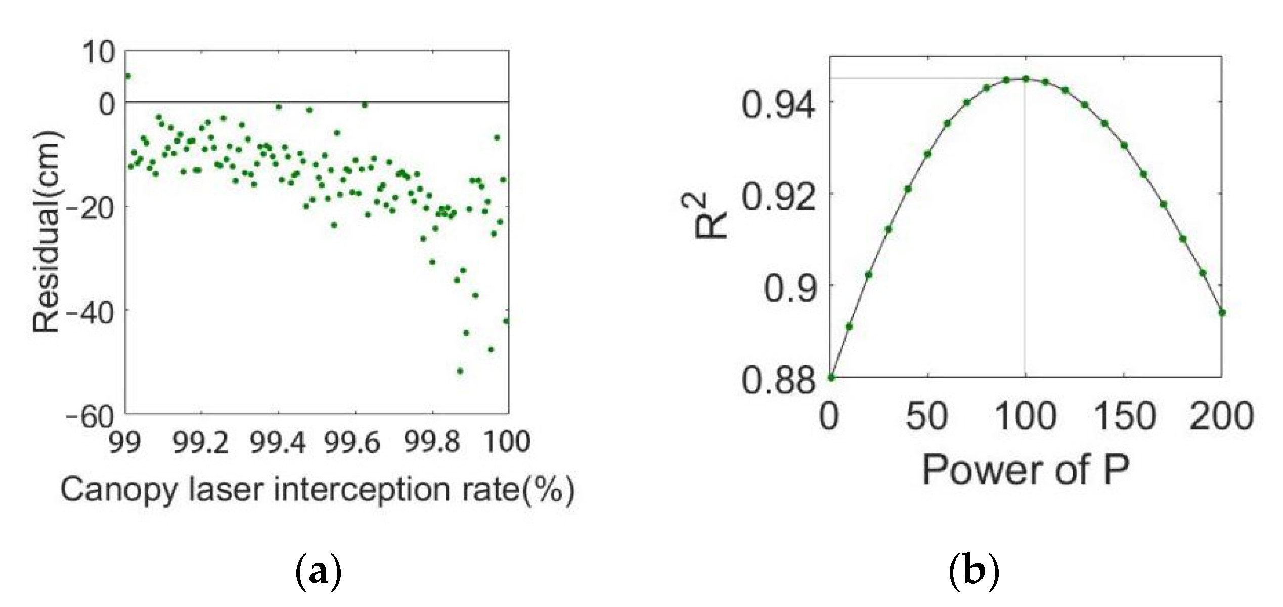
As can be seen, it is not appropriate to use a globally unified compensation coefficient, which will lead to negative optimization in the region with a low canopy interception rate and increase the estimation error. Therefore, it is a more reasonable solution to determine the compensation coefficient according to P. According to the results of Table 3, the difference in accuracy before and after compensation in the region of more than 99% canopy interception rate is the largest, but the p-value is only 1% above and below, so the primary function may not be the best fitting method. From the residual diagram of the P99 dataset (Figure 15a), it can be seen that the estimation error tends to increase rapidly when P is close to 100%, which is very close to the trend of the power function on (0, 1). The trial-and-error method is used to determine the power of P in the estimation equation. The result is shown in Figure 15b; when the power of P is 100, it is optimal, and R2 is 0.94. Finally, the estimation equation for cotton height is defined as a piecewise function, as shown in Equation (7).
H = H L i D A R ( P 98 % ) H L i D A R + 0.08 × P ( 98 % < P 99 % ) H L i D A R + 20.42 × P 100 ( 99 % < P 100 % )

3.4. Verification and Visualization

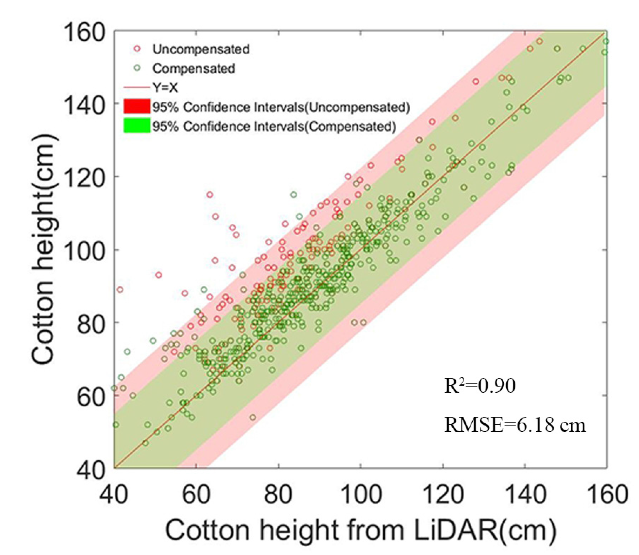
Figure 16 shows how well the estimated results match the sampling results after compensation with the canopy laser interception rate and compares them with those before compensation. Compared to the estimation accuracy before compensation, there was a significant improvement in overall R2 and RMSE, which increased by 13.92% and 45.41%, respectively (Figure 16).
Using Geographic Information System (GIS) technology, the output values of the estimation model can be mapped to the corresponding geographic locations, resulting in a crop height distribution map at the field scale (Figure 17). This can be used to observe the distribution of height differences within the field. By setting the crop height at each point on the GIS map, you can quickly and intuitively obtain the crop height distribution in the area where these points are located. In addition, using GIS software, you can calculate the median, standard deviation, minimum, and maximum values of crop height in each region, providing more accurate data support for agricultural production and management.

4. Discussion

4.1. Estimation of Canopy Height Based on Airborne LiDAR

The dense point cloud data obtained by low-altitude UAV-LiDAR includes rich canopy information and bare soil information, which has great advantages in extracting morphological features, such as canopy height. Compared with point cloud data obtained by motion recovery structure algorithm (SFM) from aerial images to measure height, the height obtained by LiDAR is more accurate, which is proved by the research of Madec et al. [26]. LiDAR point clouds can provide bare soil DEMs more easily compared to other methods, even in areas with high canopy density. This study proposes a compensation algorithm that achieves satisfactory accuracy without the need to collect a bare soil DEM before seeding, requiring only one flight. Although in Wu’s study, the generation of point clouds based on aerial oblique photography requires only one data collection, and the estimated R2 reaches 0.91, it requires the measured ground elevation interpolation to generate DEM, which will greatly increase the ease of use of the estimation model [27].
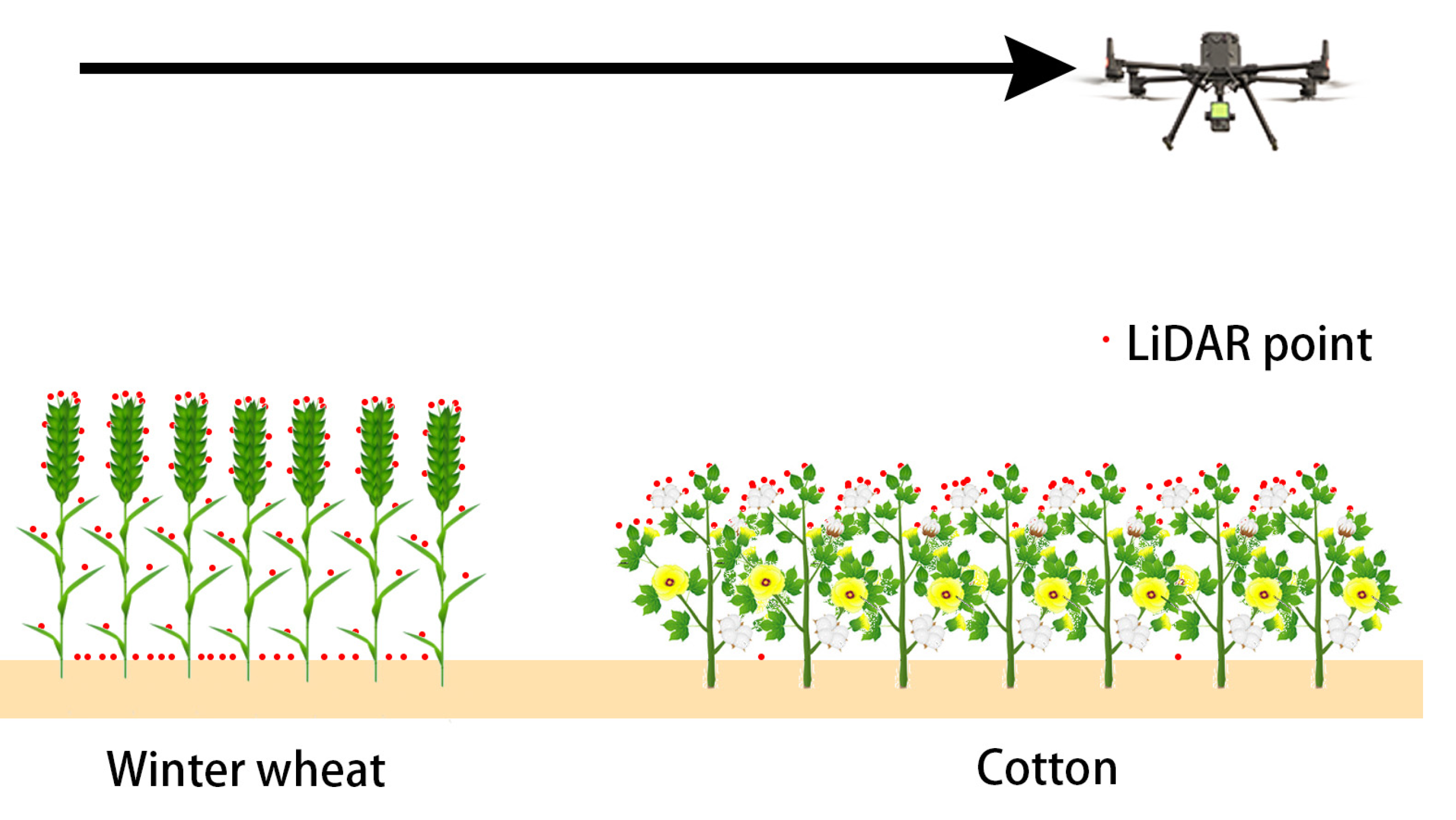
The accuracy of height estimation has much to do with the canopy structure of the crops studied, and it is easier to obtain higher estimation accuracy with a simple canopy structure (such as winter wheat height RMSE = 3.4 cm) [28]. However, the canopy structure of cotton is more complex, the planting density is very high, and the accuracy of direct measurement of canopy height is not ideal (RMSE = 10 cm) [22], mainly due to the scarcity of ground points due to the closed canopy, which makes it impossible to obtain high-quality DEM (Figure 18). In high canopy density conditions, the PTD ground filtering algorithm has significant advantages over CSF, but in situations where the number of ground points is extremely low, it may still lead to a bias in the extracted ground surface grid. Compensation of the measurement results combined with canopy laser interception rate compensation can improve this situation to a certain extent and achieve high estimation accuracy (R2 = 0.90, RMSE = 6.18 cm). It provides a solution for obtaining crop canopy height using airborne LiDAR in a single flight under high planting densities.
This study did not consider the influence of the flight height of the drone and the density of the LiDAR point cloud on the compensation function f (α) when collecting the data. In the next research plan, we will explore the influence of point cloud density and flight height on the accuracy of this research method, expand the research object to more high planting density crops, and continuously expand the applicable objects and scenarios of this research.

4.2. Application Prospect

The experimental results of this study verify the possibility of the UAV-borne LiDAR system to obtain the height of crops in a single flight under the condition of high canopy density. Compared with the traditional method of collecting the elevation of bare soil before planting [29], the method adopted in this research is easier to use and less difficult for data collection. The results of this study have important practical implications for improving the efficiency of cotton breeding research, especially in breeding experiments involving thousands of samples. The data for each community in traditional breeding experiments are usually determined by manual sampling [4], which requires many labor costs, and the results are greatly affected by human factors. The method used in this study can generate a mean value of the overall height of each community, which is more representative than manual sampling results (Figure 19), and the data collection efficiency is multiplied.
The canopy laser interception rate is highly correlated with canopy density, so its application can be tried in the quantitative inversion of leaf area index (LAI), biomass, and other traits. In addition, the fusion application of LiDAR and spectral information will become an inevitable trend in the development of research related to crop phenotype monitoring [30]; LiDAR can collect rich three-dimensional morphological data, while hyperspectral and multispectral can invert the content of some essential nutrients in crops, such as protein content [31], nitrogen content [32], chlorophyll content [33], etc. The two complement each other and lay a theoretical foundation for building a high-efficiency, high-throughput, and high-accuracy crop phenotype acquisition platform.

5. Conclusions

In this study, a new method is proposed to compensate for the canopy height estimation by using the canopy laser interception rate. The ground filtering algorithm is used to extract the ground points and calculate the interception rate of the canopy to the laser per unit volume so as to characterize the canopy density and compensate for the estimated cotton height. Through the analysis of the canopy laser interception rate step by step, the appropriate segmented height compensation function is determined, and the generation of a canopy height distribution diagram in the field is combined with GIS technology implementation. The main conclusions are summarized as follows:
(1)
The effect of the PTD ground filtering algorithm (R2 = 0.79) is significantly better than that of CSF (R2 = 0.29). The preliminary inference is that the “tip” formed by the laser penetrating the canopy can easily pass through the gaps between the fabric particles, resulting in the result obtained by the CSF filtering being the lower surface of the canopy rather than the ground;
(2)
When the canopy interception rate is greater than 99%, the estimation accuracy of LiDAR decreases sharply (R2 = 0.79, RMSE = 17.22 cm), and there is an overall trend of smaller; this is due to the lack of ground points in the sampling area, which leads to the high generated ground mesh, thus affecting the estimation accuracy;
(3)
It is not appropriate to use a globally unified compensation coefficient, which will lead to negative optimization in the area with a low canopy interception rate and increase the estimation error. Therefore, this study designs the compensation function according to the classification of canopy laser interception rate. Compared with the estimation accuracy before compensation, the overall R2 and RMSE reach 0.90 and 6.18 cm, and the results before compensation are greatly improved (R2 increase by 13.92%, RMSE decrease by 45.41%).

Author Contributions

The contributions of the authors involved in this study are as follows: W.X.: conceptualization, data curation, formal analysis, methodology, supervision, investigation, writing—original draft, and writing—review and editing; W.Y.: data curation, formal analysis, methodology, software, validation, visualization, writing—original draft, and writing—review and editing; J.W.: methodology and investigation; P.C.: methodology and investigation; Y.L.: conceptualization, funding acquisition, project administration, software, supervision, and writing—review and editing and L.Z.: conceptualization, methodology, supervision. W.X. and W.Y. contributed equally to this work. All authors have read and agreed to the published version of the manuscript.

Funding

This research was supported by the China Agriculture Research System (CARS-15-22), the Science and Technology Planning Project of Guangdong Province (2017B010117010), The 111 Project (D18019), and the Science and Technology Planning Project of Guangzhou (201807010039).

Data Availability Statement

The data used in this study are available from the corresponding author upon reasonable request.

Conflicts of Interest

The authors declare no conflict of interest.

References

  1. Araus, J.L.; Cairns, J.E. Field high-throughput phenotyping: The new crop breeding frontier. Trends Plant Sci. 2014, 19, 52–61. [Google Scholar] [CrossRef] [PubMed]
  2. Xu, W.; Chen, P.; Zhan, Y.; Chen, S.; Zhang, L.; Lan, Y. Cotton yield estimation model based on machine learning using time series UAV remote sensing data. Int. J. Appl. Earth Obs. Geoinf. 2021, 104, 102511. [Google Scholar] [CrossRef]
  3. Lati, R.N.; Filin, S.; Eizenberg, H. Plant growth parameter estimation from sparse 3D reconstruction based on highly-textured feature points. Precis. Agric. 2013, 14, 586–605. [Google Scholar] [CrossRef]
  4. Wu, J.; Mao, L.L.; Tao, J.C.; Wang, X.X.; Zhang, H.J.; Xin, M.; Shang, Y.Q.; Zhang, Y.A.; Zhang, G.H.; Zhao, Z.T.; et al. Dynamic Quantitative Trait Loci Mapping for Plant Height in Recombinant Inbred Line Population of Upland Cotton. Front. Plant Sci. 2022, 13, 914140. [Google Scholar]
  5. Xu, W.; Yang, W.; Chen, S.; Wu, C.; Chen, P.; Lan, Y. Establishing a model to predict the single boll weight of cotton in northern Xinjiang by using high resolution UAV remote sensing data. Comput. Electron. Agric. 2020, 179, 105762. [Google Scholar] [CrossRef]
  6. Cheng, J.P.; Yang, H.; Qi, J.B.; Sun, Z.D.; Han, S.Y.; Feng, H.K.; Jiang, J.Y.; Xu, W.M.; Li, Z.H.; Yang, G.J.; et al. Estimating canopy-scale chlorophyll content in apple orchards using a 3D radiative transfer model and UAV multispectral imagery. Comput. Electron. Agric. 2022, 202, 107401. [Google Scholar]
  7. Tahir, M.N.; Lan, Y.; Zhang, Y.; Wang, Y.; Nawaz, F.; Shah, M.A.A.; Gulzar, A.; Qureshi, W.S.; Naqvi, S.M.; Naqvi, S.Z.A. Real time estimation of leaf area index and groundnut yield using multispectral UAV. Int. J. Precis. Agric. Aviat. 2020, 1, 1–6. [Google Scholar]
  8. Kawamura, K.; Asai, H.; Yasuda, T.; Khanthavong, P.; Soisouvanh, P.; Phongchanmixay, S. Field phenotyping of plant height in an upland rice field in Laos using low-cost small unmanned aerial vehicles (UAVs). Plant Prod. Sci. 2020, 23, 452–465. [Google Scholar] [CrossRef]
  9. Malachy, N.; Zadak, I.; Rozenstein, O. Comparing Methods to Extract Crop Height and Estimate Crop Coefficient from UAV Imagery Using Structure from Motion. Remote Sens. 2022, 14, 810. [Google Scholar] [CrossRef]
  10. Holman, F.H.; Riche, A.B.; Michalski, A.; Castle, M.; Wooster, M.J.; Hawkesford, M.J. High Throughput Field Phenotyping of Wheat Plant Height and Growth Rate in Field Plot Trials Using UAV Based Remote Sensing. Remote Sens. 2016, 8, 1031. [Google Scholar] [CrossRef]
  11. Luo, S.Z.; Liu, W.W.; Zhang, Y.Q.; Wang, C.; Xi, X.H.; Nie, S.; Ma, D.; Lin, Y.; Zhou, G.Q. Maize and soybean heights estimation from unmanned aerial vehicle (UAV) LiDAR data. Comput. Electron. Agric. 2021, 182, 106005. [Google Scholar]
  12. Ni-Meister, W.; Yang, W.Z.; Lee, S.; Strahler, A.H.; Zhao, F. Validating modeled lidar waveforms in forest canopies with airborne laser scanning data. Remote Sens. Environ. 2018, 204, 229–243. [Google Scholar]
  13. Xu, P.; Wang, H.; Yang, S.; Zheng, Y. Detection of crop heights by UAVs based on the Adaptive Kalman Filter. Int. J. Precis. Agric. Aviat. 2021, 1, 52–58. [Google Scholar] [CrossRef]
  14. Yang, H.; Hu, X.; Zhao, J.; Hu, Y. Feature extraction of cotton plant height based on DSM difference method. Int. J. Precis. Agric. Aviat. 2021, 1, 59–69. [Google Scholar] [CrossRef]
  15. Chen, G.; Hay, G.J. An airborne lidar sampling strategy to model forest canopy height from Quickbird imagery and GEOBIA. Remote Sens. Environ. 2011, 115, 1532–1542. [Google Scholar]
  16. Qiu, Q.; Sun, N.; Bai, H.; Wang, N.; Fan, Z.Q.; Wang, Y.J.; Meng, Z.J.; Li, B.; Cong, Y. Field-Based High-Throughput Phenotyping for Maize Plant Using 3D LiDAR Point Cloud Generated With a “Phenomobile”. Front. Plant Sci. 2019, 10, 554. [Google Scholar] [CrossRef] [PubMed]
  17. Schaefer, M.T.; Lamb, D.W. A Combination of Plant NDVI and LiDAR Measurements Improve the Estimation of Pasture Biomass in Tall Fescue (Festuca arundinacea var. Fletcher). Remote Sens. 2016, 8, 109. [Google Scholar] [CrossRef]
  18. Eitel, J.; Magney, T.S.; Vierling, L.A.; Brown, T.T.; Huggins, D.R. LiDAR based biomass and crop nitrogen estimates for rapid, non-destructive assessment of wheat nitrogen status. Field Crops Res. 2014, 159, 21–32. [Google Scholar] [CrossRef]
  19. Watanabe, K.; Guo, W.; Arai, K.; Takanashi, H.; Kajiya-Kanegae, H.; Kobayashi, M.; Yano, K.; Tokunaga, T.; Fujiwara, T.; Tsutsumi, N.; et al. High-Throughput Phenotyping of Sorghum Plant Height Using an Unmanned Aerial Vehicle and Its Application to Genomic Prediction Modeling. Front. Plant Sci. 2017, 8, 421. [Google Scholar] [CrossRef]
  20. Oh, S.; Jung, J.; Shao, G.; Shao, G.; Gallion, J.; Fei, S. High-Resolution Canopy Height Model Generation and Validation Using USGS 3DEP LiDAR Data in Indiana, USA. Remote Sens. 2022, 14, 935. [Google Scholar] [CrossRef]
  21. Lou, S.W.; Dong, H.Z.; Tian, X.L.; Tian, L.W. The “Short, Dense and Early” Cultivation of Cotton in Xinjiang: History, Current Situation and Prospect. Sci. Agric. Sin. 2021, 54, 720–732. [Google Scholar]
  22. Xu, R.; Li, C.Y.; Bernardes, S. Development and Testing of a UAV-Based Multi-Sensor System for Plant Phenotyping and Precision Agriculture. Remote Sens. 2021, 13, 3517. [Google Scholar] [CrossRef]
  23. Yan, P.C.; Han, Q.S.; Feng, Y.M.; Kang, S.Z. Estimating LAI for Cotton Using Multisource UAV Data and a Modified Universal Model. Remote Sens. 2022, 14, 4272. [Google Scholar] [CrossRef]
  24. Axelesson, P.E. DEM Generation from Laser Scanner Data Using Adaptive TIN Models. Int. Arch. Photogramm. Remote Sens. Spat. Inf. Sci. 2000, 4, 110–117. [Google Scholar]
  25. Zhang, W.M.; Qi, J.B.; Wan, P.; Wang, H.T.; Xie, D.H.; Wang, X.Y.; Yan, G.J. An Easy-to-Use Airborne LiDAR Data Filtering Method Based on Cloth Simulation. Remote Sens. 2016, 8, 501. [Google Scholar] [CrossRef]
  26. Madec, S.; Baret, F.; de Solan, B.; Thomas, S.; Dutartre, D.; Jezequel, S.; Hemmerle, M.; Colombeau, G.; Comar, A. High-Throughput Phenotyping of Plant Height: Comparing Unmanned Aerial Vehicles and Ground LiDAR Estimates. Front. Plant Sci. 2017, 8, 2002. [Google Scholar] [CrossRef]
  27. Wu, J.; Wen, S.; Lan, Y.; Yin, X.; Zhang, J.; Ge, Y. Estimation of cotton canopy parameters based on unmanned aerial vehicle (UAV) oblique photography. Plant Methods 2022, 18, 129. [Google Scholar]
  28. Ten Harkel, J.; Bartholomeus, H.; Kooistra, L. Biomass and Crop Height Estimation of Different Crops Using UAV-Based Lidar. Remote Sens. 2020, 12, 17. [Google Scholar] [CrossRef]
  29. Bendig, J.; Bolten, A.; Bennertz, S.; Broscheit, J.; Eichfuss, S.; Bareth, G. Estimating Biomass of Barley Using Crop Surface Models (CSMs) Derived from UAV-Based RGB Imaging. Remote Sens. 2014, 6, 10395–10412. [Google Scholar] [CrossRef]
  30. Roitsch, T.; Cabrera-Bosquet, L.; Fournier, A.; Ghamkhar, K.; Jimenez-Berni, J.; Pinto, F.; Ober, E.S. Review: New sensors and data-driven approaches-A path to next generation phenomics. Plant Sci. 2019, 282, 2–10. [Google Scholar]
  31. Tan, C.; Zhou, X.; Zhang, P.; Wang, Z.; Wang, D.; Guo, W.; Yun, F. Predicting grain protein content of field-grown winter wheat with satellite images and partial least square algorithm. PLoS ONE 2020, 15, e0228500. [Google Scholar]
  32. Feng, S.; Cao, Y.; Xu, T.; Yu, F.; Chen, C.; Zhao, D.; Jin, Y. Inversion Based on High Spectrum and NSGA2-ELM Algorithm for the Nitrogen Content of Japonica Rice Leaves. Spectrosc. Spectr. Anal. 2020, 40, 2584–2591. [Google Scholar]
  33. Zhang, L.Y.; Han, W.T.; Niu, Y.X.; Chavez, J.L.; Shao, G.M.; Zhang, H.H. Evaluating the sensitivity of water stressed maize chlorophyll and structure based on UAV derived vegetation indices. Comput. Electron. Agric. 2021, 185, 106174. [Google Scholar]
Figure 1. Study site location.
Agronomy 13 02584 g001
Figure 2. (a) Height measurement, (b) geographic location record, and (c) sampling data overview.
Agronomy 13 02584 g002
Figure 3. The technical approach used in this study.
Agronomy 13 02584 g003
Figure 4. (a) M300 RTK and ZENMUSE L1, (b) Shihezi Route and (c) Jiujiang Route.
Agronomy 13 02584 g004
Figure 5. Overlapping area redundancy data elimination in navigation belt.
Agronomy 13 02584 g005
Figure 6. TIN construction method.
Agronomy 13 02584 g006
Figure 8. CSF Algorithm Principle Illustration.
Agronomy 13 02584 g008
Figure 9. Cloth particle movement process.
Agronomy 13 02584 g009
Figure 10. High interpolation ground grid phenomenon.
Agronomy 13 02584 g010
Figure 11. Canopy laser interception rate grid.
Agronomy 13 02584 g011
Figure 12. (a) Scatter plot and (b) residual plot.
Agronomy 13 02584 g012
Figure 13. Ground grid section view (Generated by PTD and CSF, Buffer zone 5 cm).
Agronomy 13 02584 g013
Figure 14. Ground grid section view (Generated by PTD and CSF).
Agronomy 13 02584 g014
Figure 15. (a) P99 residual diagram and (b) the relationship between the power of P and R2.
Agronomy 13 02584 g015
Figure 16. Height estimation model accuracy of canopy interception rate compensation.
Agronomy 13 02584 g016
Figure 17. Canopy height distribution in Shihezi research area, Xinjiang (left) and Jiujiang research area, Jiangxi (right).
Agronomy 13 02584 g017
Figure 18. Comparison of canopy structure between winter wheat and cotton.
Agronomy 13 02584 g018
Figure 19. Examples of application in breeding experiments.
Agronomy 13 02584 g019
Table 1. Parameters of remote sensing data acquisition equipment.
ZENMUSE L1
LiDAR
Ranging accuracy3 cm at 100 m
Maximum number of echoes supported3
FOVRepeat scanning: 70.4° × 4.5°
Non Repeat scanning: 70.4° × 77.2°
Data acquisition rateSingle echo: 240,000 points/s
Multi echo: 480,000 points/s
IMU (Inertial Measurement Unit)
Refresh rate200
Course Accuracy; Pitch accuracy0.15°; 0.025°
RGB Camera
Resolution of CMOS sensor5472 × 3648
Focal length8.8 mm/24 mm (Equivalent full frame)
Aperturef/2.8–f/11
Table 2. P90, P95, P97, P98, and P99 data overview. H represents height, and P represents the canopy laser interception rate in the sampling area.
DatasetSample SizeMean (H)Std (H)Mean (P)Std (P)
Total44084.28 cm20.61 cm88%18.20%
P70 (70–90%)6285.63 cm22.82 cm81%5.65%
P90 (90–95%)3286.94 cm17.82 cm92%1.37%
P95 (95–97%)4390.49 cm21.43 cm95%0.59%
P97 (97–98%)3784.76 cm21.27 cm97%0.29%
P98 (98–99%)7187.38 cm17.21 cm98%0.29%
P99 (99–100%)12484.25 cm19.18 cm99%0.30%
Table 3. The difference in estimation accuracy of canopy interception rate before and after compensation.
DatasetEstimating EquationR2RMSE (cm)R2 Groth RateRMSE Reduction Rate
TotalHLiDAR + 6.97 × P0.779.43−2.53%15.81%
P70 (70–90%)HLiDAR + 2.24 × P0.897.490%−0.13%
P90 (90–95%)HLiDAR + 1.18 × P0.866.763.61%8.15%
P95 (95–97%)HLiDAR + 0.58 × P0.925.971.10%8.58%
P97 (97–98%)HLiDAR − 1.43 × P0.916.321.11%0.94%
P98 (98–99%)HLiDAR + 0.08 × P0.944.122.17%35.82%
P99 (99–100%)HLiDAR + 14.86 × P0.886.4611.40%62.49%
Disclaimer/Publisher’s Note: The statements, opinions and data contained in all publications are solely those of the individual author(s) and contributor(s) and not of MDPI and/or the editor(s). MDPI and/or the editor(s) disclaim responsibility for any injury to people or property resulting from any ideas, methods, instructions or products referred to in the content.